Abstract
The effect of the number of waves and the width of the ridge and valley in chord direction for a wavy airfoil was investigated at the angle of attack of and Reynolds number of through using the two-dimensional direct numerical simulation for four kinds of wavy airfoil shapes. A new method for parameterizing a wavy airfoil was proposed. In comparison with the original corrugated airfoil profile, the wavy airfoils that have more distinct waves show a lower aerodynamic efficiency and the wavy airfoils that have less distinct waves show higher aerodynamic performance. For the breakdown of the lift and drag concerning the pressure stress and friction stress contributions, the pressure stress component is significantly dominant for all wavy airfoil shapes concerning the lift. Concerning the drag, the pressure stress component is about for the wavy airfoils that have more distinct waves, while the frictional stress component is about for the wavy airfoils that have less distinct waves. From the distribution of pressure isoline and streamlines around wavy airfoils, it is confirmed that the pressure contributions of the drag are dominant due to high pressure on the upstream side and low pressure on the downside; the frictional contribution of the drag is dominant due to large surface areas of the airfoil facing the external flow. The effect of the angle of attack on the aerodynamic efficiency for various wavy airfoil geometries was studied as well. Aerodynamic shape optimization based on the continuous adjoint approach was applied to obtain as much as possible the highest global aerodynamic efficiency wavy airfoil shape. The optimal airfoil shape corresponds to an increase of and over the aerodynamic efficiency and the lift from the initial geometry, respectively, when optimal airfoil has an approximate drag coefficient compared to the initial geometry. Concerning an fixed angle of attack, the optimal airfoil is statically unstable in the range of the angle of attack from to , statically quasi-stable from to , where the vortex is shedding at the optimal airfoil leading edge. Concerning an angle of attack passively varied due to the fluid force, the optimal airfoil keeps the initial angle of attack value with an initial disturbance, then quickly increases the angle of attack and diverges in the positive direction.
1. Introduction
Recently, micro-air vehicles (MAVs) [1], nano-air vehicles (NAVs) [2], and pico-air vehicles (PAVs) [3] have been widely used by researchers, security and law enforcement agencies, search and rescue operators, firefighters, farmers, filmmakers, photographers, and delivery companies. Motivated by the enormous global appetite for applying MAVs, NAVs, and PAVs, the design of high aerodynamic performance airfoils for these applications has received considerable attention in recent years. Micro-, nano-, and pico-air vehicles are working at low Reynolds number () [4,5]. In particular, it is worth mentioning Defense Advanced Research Projects Agency (DARPA) specifications for NAVs with an extremely small wingspan <7.5 cm and working at , and PAVs working at [6]. Thus, the study of aerodynamics and shape optimization for airfoils at ultra-low Reynolds numbers becomes pertinent for engineered flying objects. For the Reynolds number region from to , various investigations of aerodynamic phenomena have appeared [5,7,8,9]. However, the databases of airfoils at Reynolds number less than this range airfoil data below this range are very limited [10,11,12,13]. Of particular interest in this study is the level of Reynold number at . Here, this Reynolds number regime is called ultra-low. Although many MAVs, NAVs, and PAVs have been designed over the last few years, the typically applied airfoil platform is still the contractible version of that applied for the giant aircraft at high Reynolds number. Due to the difference between the high Reynold number regime and the ultra-low Reynolds number regime, such as the dominant inertial force for the high Reynold number regime but dominant viscous force for the ultra-low Reynold number regime, the optimal airfoil design for the giant aircraft might be distinguished momentously from that for MAVs, NAVs, and PAVs. Therefore, there is an important requirement to readjust the typical streamlines airfoil platform for ultra-low Reynolds numbers regime.
One way of designing effective airfoils at ultra-low Reynolds number is by biomimetics [5,14,15,16]. The dragonfly is considered as a high-performance flyer. The typical range of the Reynolds number for dragonflies is from 100 to [17], which can be categorized as the ultra-low Reynolds number flow regime. Dragonflies have both gliding and flapping flight modes. When flapping, they can suddenly accelerate and stop, hover, and turn [18]. In gliding flight, the dragonfly elevates into the air using powered (flapping) flight and makes use of potential energy to move horizontally above the ground [19,20]. It is generally known that the dragonfly has highly corrugated wings where the wing’s cross-section varies along the chordwise direction, as seen in Figure 1, unlike that of a typical engineered airfoil which is streamlined and smooth cambered. Extensive biological and aerodynamic studies of corrugated airfoils have been carried out by many researchers [18,21,22,23,24,25,26]. Visualization of the two-dimensional flow field around the blade cross section using a bent airfoil has been made by Komine [27]. Our previous study has conducted numerical analysis of the two- and three-dimensional flow fields around the corrugated airfoil and quantitative evaluation of the aerodynamic characteristics [28]. It has been found that the corrugated airfoil performs significantly better than the streamlined airfoil at ultra-low Reynolds number with the low angle of attacks, and performs as well at the high angle of attacks.
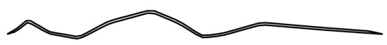
Figure 1.
A corrugated airfoil.
There are several attempts to explain the reason of the unexpected improvement in the aerodynamic performance for the corrugated airfoil at ultra-low Reynolds number. One explanation is that air flow over the airfoil corrugations is trapped between the valleys and essentially forms a virtual streamlined airfoil [20,23]. Another explanation is that the delay of the flow separation or the earlier reattachment of the flow separation for the corrugated airfoil corresponds to the improved performance [18,25]. In spite of different explanations for the improved aerodynamic performance, these studies unanimously agree that the corrugated airfoil performs well in ultra-low Reynolds number regimes. Thus, such corrugated airfoils could be candidates for MAVs, NAVs, and PAVs. Since the dragonfly’s flight forms include flapping and glide, the corrugated airfoil shape can be considered to have been optimized for multiple purposes. Research on flapping using corrugated wing has been conducted by experiments and numerical calculations from the viewpoint of developing MAVs, NAVs, and PAVs [29,30,31]. Flapping wings are said to be able to obtain higher thrust than gliding wings, but application issues such as complicated mechanisms results in increased weight and less flight time. For fixed wing MAV, NAVs, and PAVs, wings that simultaneously provide a superior aerodynamic performance and structural robustness are critical. However, there is no guarantee that wing sections like dragonflies are optimized for aerodynamic characteristics during gliding. Therefore, in order to obtain an airfoil shape that exhibits higher aerodynamic performance in gliding at ultra-low Reynolds number, aerodynamic shape optimization for a corrugated airfoil of dragonflies is necessary.
Over the past several decades, aerodynamic shape optimization has been successfully applied for two-dimensional and simple three-dimensional configurations. General aerodynamic shape optimization includes a global method based on a heuristic algorithm and gradient method. The global optimization method is a probabilistic method that simulates biological phenomena and physical phenomena, as represented by genetic algorithms [32], artificial neural networks [33], and response surface method [34]. This method can search for solutions without convergence to local solutions even when the objective function has multimodality. However, it takes up huge amounts of computational resources and is time-consuming to obtain an optimal solution. On the other hand, researchers [35] found efficient global optimization of expensive black-box functions by using response surfaces for global optimization lies in balancing the need to exploit the approximating surface with the need to improve the approximation. For the gradient-based aerodynamic shape optimization, through simplifying the description of real-life problems, the optimal solution is searched by analytically finding the gradient vector and Hessian matrix related to the design variables concerning the objective function. In particular, adjoint-based methods [36,37,38,39,40] seem to be an attractive alternative, since the sensitivity analysis is independent of the number of design variables and proportional to the number of aerodynamic cost functions. In addition, the cost function gradient concerning the design variables is calculated indirectly by solving the flow governing equations and the adjoint equation, in which the cost of calculating the adjoint equation is almost the same as that of solving the flow equations. Based on the order of discretization and derivation of the adjoint equations, the adjoint-based method can be further classified as continuous and discrete. The advantage of the continuous adjoint method is that it is independent of the method used to solve the flow equations. Adjoint-based methods have been utilized in diverse areas such as aerospace [41,42], marine [43], and biomedical engineering [44]. In addition, they have been used to design optimal airfoil [6,39,43,45,46,47]. In this study, an aerodynamic shape optimization procedure for a corrugated airfoil of dragonflies using a continuous adjoint method is implemented. A time marching finite difference method is utilized to solve the flow and adjoint equations. The properties of the adjoint equations are very similar to the flow equations, thus many numerical schemes for flow solvers can be applied to the adjoint solvers as well. The simple steepest descent algorithm is employed to minimize the objective function.
By the way, many of these studies treat wings as rigid bodies. Naka and Hashimoto have conducted experiments using a wing model of an elastic film and a rigid rod that reproduces the deformation of a dragonfly wing when flapping and gliding flight [48,49]. Numerical calculations using this wing model are also performed for glide, and the flow is left by deforming the wing so that it twists around the span direction axis. It is clear that the drag coefficient reduction rate is increased more than that of the lift coefficient, resulting in a higher lift-drag ratio than the rigid wing. Numerical calculation of the corrugated airfoil considering deformation is also important for evaluating the strength of wing for receiving force from fluid. In particular, when handling a rigid three-dimensional corrugated wing, it is predicted that the moment of force around the root of the wing will be larger than that of an elastic wing. At present, few studies have been conducted to evaluate and compare the hydrodynamic force and moment of force acting in each case where the corrugated wing during flight is an elastic body and a rigid body. Therefore, in this study, the hydrodynamic moment of force and the attitude stability of the optimal airfoil for ultra-low Reynolds number regime in gliding flight is investigated as well.
One objective of this study is to conduct a systematic investigation to study the improvement in aerodynamic performance for a series of wavy airfoil profiles generated by modifying the number of waves and the width of the ridge and valley in the chord direction. A novel scheme is proposed to represent corrugations, that is, the width of the ridge and valley of a wavy airfoil in the chord direction is expressed by the wavenumber of the sine wave. The height of the wave in the chord direction is limited by the envelope of the aircraft airfoil NACA20408. First, the effect of the number of waves and the width of the ridge and valley on the lift coefficient, drag coefficient, and the aerodynamic efficiency are investigated through intentionally changing waves for the airfoil. Various cases are considered. The number, width, and height of waves are varied on the whole airfoil, while the thickness of the wavy airfoil is fixed at of the chord length. The effect of the angle of attack on the aerodynamic efficiency for various wavy airfoil geometries is studied as well.
Another objective of this study is to optimize the waves for high aerodynamic performance (in terms of lift-to-drag ratio) using a continuous adjoint method. The aerodynamic shape optimization is conducted on a high aerodynamic efficiency wavy airfoil, in which the NACA2408 airfoil is used as the envelope for the height of corrugations. Performance of the optimized wavy airfoil, the original corrugated airfoil, and NACA2408 airfoil are compared. Due to our application pointing to ultra-low Reynolds number regime in gliding flight, the Reynolds number and angle of attack for the optimization is and , respectively. The flow governing equations and the adjoint equations are calculated through a time-marching finite difference method. The minimizations of the objective function are carried out by using the steepest descent algorithm.
The third objective of the present paper is to evaluate the hydrodynamic moment of force and the attitude stability of the optimal airfoil for ultra-low Reynolds number regime in gliding flight is investigated as well. There are two applied problem settings. One is that the angle of attack of the optimal wavy airfoil, the original corrugated airfoil, and NACA2408 airfoil are fixed to discuss the hydrodynamic moment of force and statically stability. Another is that the angle of attack of the optimal wavy airfoil is passively changed by the fluid force to study the attitude stability.
2. Computational Methodology
In this study, there are two applied problem settings. One is that the angle of attack of the airfoil is fixed to investigated the improvement in aerodynamic performance for a series of wavy airfoil profiles generated by modifying the number of waves and the width of the ridge and valley in the chord direction and optimize the waves for high aerodynamic efficiency using a continuous adjoint method. The computational theory for the first problem setting is introduced in Section 2.1, Section 2.2 and Section 2.3. Another is that the angle of attack of the airfoil is passively changed by the fluid force to analyze the attitude stability. For the latter, a moving grid technical adapted to the moving airfoil surface is applied. The computational theory for the second problem setting is introduced in Section 2.4. More details of computation of the attitude stability of airfoil are described in our previous studies [28].
2.1. Flow Equations
This section presents the flow governing equations for numerically calculating the flow field over the airfoil. Consider a domain , with boundary that is spatial and temporal and occupied by a fluid of density and dynamic viscosity . The spatial and temporal coordinates are denoted by and t. For the incompressible Newtonian fluid, the continuity equation and the Navier–Stokes equations can be represented as
where means the velocity, p denotes the pressure, and is identity tensor. The boundary conditions are either on the flow velocity or stress. Both Dirichlet and Neumann-type boundary conditions are considered:
Here, is the unit normal vector on the boundary . and are the subsets of the boundary . The boundary can be further split, such as , , and are the upstream, downstream, and lateral boundaries, respectively, and is the body surface. The initial velocity condition can be written as
Here, indicates divergence free. The drag and lift force coefficient, (, ), on the body are calculated using the following expression:
The time-averaged drag and lift coefficients can be computed from:
Note that the time should start at until the flow is fully developed and the time interval for averaging T should be large enough so that the mean value is stationary.
2.2. The Continuous Adjoint-Based Aerodynamic Optimization Method
The continuous adjoint-based aerodynamic optimization method is presented in this section. Let be the segment of the boundary , whose shape is to be determined by the set of parameters …. Let be the objective, in which the independent variables includes the flow variables and shape parameters . Thus, minimizing the objective function , the shape parameters are determined in the optimization procedure. When makes a small change, a corresponding small change of appears. Namely,
The flow Equations (1) and (2) can be written as , which expresses the dependence on and and seems to exist as the constraint conditions for the objective function . Then, can be written. Thus, can be determined from
An augmented objective function is constructed to convert the constrained problem into an unconstrained one. The flow equations are augmented to the original objective function by introducing a set of Lagrange multipliers or adjoint variables :
If the flow variables, , exactly satisfy the flow Equations (1) and (2), the augmented objective function (11) degenerates to the objective function . Then, the first variation of the augmented objective function (9) can be written as follows:
where
Moreover, since the variation in is zero, it can be multiplied by and subtracted from the variation without changing the result. Thus, Equation (12) can be written as
Here, should be carefully selected and satisfy the adjoint equations:
Substitution of the adjoint Equation (17) into Equation (16) results in the following equation for and .
where
From the above equation, an optimal solution of shape parameters can be obtained as the gradient of the augmented objective function reaches 0, i.e., . Thus, the gradient given by Equation (19) is utilized to find the optimal shape parameters. Since the gradient is independent of , the gradient of with respect to an arbitrary number of design variable can be determined with the need for additional flow field evaluations. The main cost is in solving the adjoint Equation (17). In general, the adjoint problem is about as complex as a flow solution. Once Equation (19) is obtained, the gradient can be fed into any numerical optimization algorithm to obtain an improved design.
2.3. The Adjoint Equations
The equation and the boundary conditions for adjoint variables can be carried out when the representation written in Equation (17) is set up. Thus, the adjoint equations can be written as:
The adjoint Equations (20) and (21) are a set of coupled linear partial differential equations. Unlike the flow Equations (1) and (2), the equations for the adjoint variables are posed backward in time. The boundary conditions on the adjoint variables are
where , means the upstream boundary, means the downstream boundary, means the lateral boundaries, and is the body surface. The terminal condition on the adjoint velocity is given by:
2.4. Attitude Stability
The basic equations are the continuity and Navier–Stokes equations for an incompressible Newtonian fluid. A non-dimensionalization is applied to all variables by means of the streamwise velocity and chord length L. Since the boundary-fitted-grid is employed in our computation, a general curvilinear coordinates has to be applied and is represented as , , . Based on the references [50,51],
where J represents the Jacobian of the coordinate transformation, means the contravariant velocity, means the Reynolds number, as in , denotes the moving speed component of the grid point in the general coordinate. In the pitching direction, the angle of attack variation because of the fluid force can be written as:
Here, means the inertia moment, and are the moment coefficient of the fluid force and the support moment coefficient in the pitching direction, where the support point of the airfoil is at the chord length from the airfoil leading edge, S denotes the effective area, and means the angle of attack, which is opposite to the direction of the fluid moment. There is therefore a negative sign is applied on the left-hand side of Equation (29).
3. Implementation Details
3.1. Shape Parameterization
The original corrugated airfoil used in this study is the same as our previous study used in numerical simulation [28]; see Figure 1. The position treated in this study is a coordinate system along the chord direction, and the position of the leading edge is defined as the origin , and the position of the trailing edge is standardized as . In order to try to explore a new form of the corrugated airfoil for gliding at ultra-low Reynolds number, as well as reduce the design variables for shape optimization, the width of the ridge or valley in the chord direction for the corrugated airfoil is expressed by the wavenumber of the sine wave. This kind of corrugated airfoil (i.e., a wavy airfoil) has different ridge and valley widths on the leading and trailing edge regions; see an example in Figure 2. Therefore, the wavenumber of the wavy airfoil is a model with the position ( ) in the chord direction as the independent variable. In this study, the wavenumber of the wavy wing is expressed by a quadratic function:
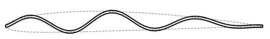
Figure 2.
A wavy airfoil.
Here, A, B, and C are constants and are determined to satisfy the following conditions:
a is the wave number at the leading edge, b is the wave number at the trailing edge, and c is the position of the quadratic function axis. From the above, the wavenumber of the corrugated wing can be expressed using the parameters a, b, and c as follows:
Next, the height of the wave for the wavy airfoil remains to be decided. Since the original corrugated airfoil has a shape with the envelope of NACA2408 airfoil as shown in Figure 3, the height of the wave is also determined by using NACA2408 airfoil as the envelope, see Figure 2. Let be the thickness of NACA2408 airfoil at the position of in the chord direction. The thickness of the wavy airfoil is fixed at of the chord length in this study. Finally, the height of the wavy airfoil can be expressed as:
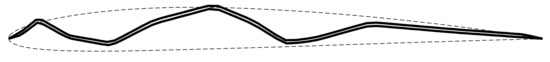
Figure 3.
A corrugated airfoil and its envelope of NACA2408 airfoil.
When has an inflection point, the wavy airfoil will not use the NACA2408 airfoil as the envelope, as shown in Figure 4. Thus, this case of existing inflection point has to be rejected. Substitute Equation (32) into Equation (33) and take the first derivative of identically equalling to zero, leading to the condition expression for the parameters a, b, and c that must satisfy as follows:
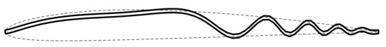
Figure 4.
The shape of a wavy airfoil that has an inflection point in the chord direction.
As a result, based on the above discussion, the shape of the wavy airfoil handed in this study is determined.
3.2. The Objective Function
When a relatively large lift coefficient and low drag coefficient are both achieved, we term this airfoil as high performance airfoil. Thus, the time-averaged aerodynamic efficiency is employed as the objective function for our optimization:
3.3. Computational Domain, Mesh, and Boundary Conditions
The computational domain and boundary conditions for corrugated airfoil and NACA2408 airfoil are shown in Figure 5, where L is the chord length of the airfoil. A Cartesian coordinate system is used to define x in the mainstream direction and y in the vertical direction. Due to the H-type boundary-fitted grid employed, a general curvilinear coordinate system has to be applied and represented as and for all computations, in which the direction following the mainstream direction is denoted as , and the direction away from the surface of airfoil is defined as . The computational mesh near the airfoil surface is shown in Figure 6. Through using the mesh moving scheme on the initial grid points, the different geometries meshes are created. In this scheme, the mesh in the flow domain is modeled as a linear elastic solid and is deformed to accommodate the new geometry of the airfoil [52,53,54]. When the angle of attack of the airfoil is passively changed by the fluid force, transfinite interpolation method is used to regenerate the grids on the moving airfoil surface [55]. The validation of the mesh convergence for evaluating the adequacy of the spatial resolution was carried out in our previous studies [28].
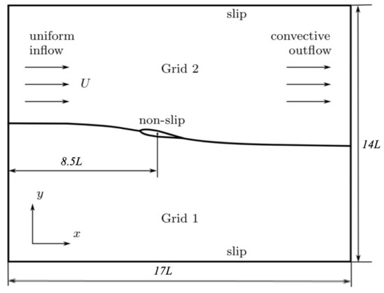
Figure 5.
Computational domain and boundary conditions.
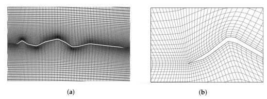
Figure 6.
Computational grid: (a) corrugated airfoil; and (b) around leading edge.
The computational domain and boundary condition are showed in Figure 5. More details are introduced in our previous article [28]. The computational parameters are summarized in Table 1. Firstly, in order to to conduct a systematic investigation to study the improvement in aerodynamic performance for a series of wavy airfoil profiles generated by modifying the number of waves and the width of the ridge and valley in the chord direction, the direct numerical simulations of the flow around different wavy airfoils are conducted with the computational parameters of in Table 1. Next, for optimizing the corrugations for high aerodynamic efficiency using a continuous adjoint method, the computational parameters of in Table 1 are used. Finally, to evaluate the attitude stability of the optimal wavy airfoil generated by using our shape optimization procedure, we perform the simulations with the computational parameters of given in Table 1.

Table 1.
Computational parameters. The superscript + means the wall unit.
3.4. Implementation of the Numerical Method and Optimization Procedure
A finite difference method is utilized to solve the flow and adjoint equations. Since the properties of the adjoint equations are very similar to the flow equations, numerical schemes for flow solvers can be applied to the adjoint solvers as well. In this study, applying a cell-centered, collocated arrangement the flow equations and adjoint equations are discretized, in which all physical variables and the corresponding contravariant components are located at the cell center and cell-face center, respectively. A 2-order spatial central finite difference discretization technique is employed. For coupling the pressure field and the continuity equation, the fractional method is applied [56]. For the time marching of the flow and adjoint equations, the 2-order Adams–Bashforth method is applied to the convective terms, the 2-order Crank–Nicolson method is used to the viscous terms in order to eliminate the viscous stability constraint, and the backward Euler method is utilized for the pressure term. For the calculation, the Poisson equation is the most time-consuming procedure and calculated through the residual cutting method [57]. This numerical technique used in this study has been validated extensively in several turbulent flows [28,58,59,60,61]. For the problem setting where the angle of attack of airfoil is passively changed by the fluid force, the 2-order Runge–Kutta method is utilized for the time marching of Equation (29).
The cycle of the aerodynamic optimization starts with an initial geometry. Then, the structured meshes for the initial geometry is produced. The numerical calculation of the flow field is conducted enough times until the flow fields were fully developed and the aerodynamic coefficients exhibit adequate convergence. The adjoint variables are calculated using the date from the last 1000 steps solution of the flow field. Then, the gradients in Equation (19) for the objective function (36) can be obtained using the solutions of the flow governing equations and adjoint equations. Through a numerical optimization algorithm, the gradient is employed to obtain an improved design. In order to accommodate a new airfoil profile, the structured mesh is adjusted through a mesh moving scheme. In Figure 7 and Figure 8, the details of an aerodynamic optimization procedure and an example of the iteration history of the present objective function are showed, where the angle of attack is and the values of the design variables for the initial geometry are . Table 2 shows the change in the value of before and after the shape optimization procedure. An improvement in the lift-to-drag ratio of approximately is confirmed after a shape optimization procedure.
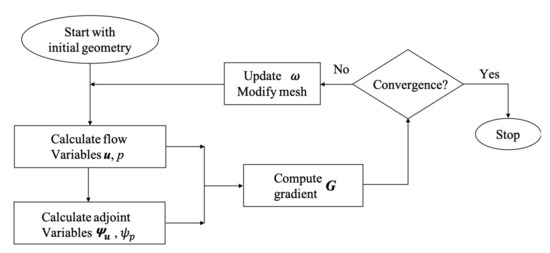
Figure 7.
Optimization procedure.
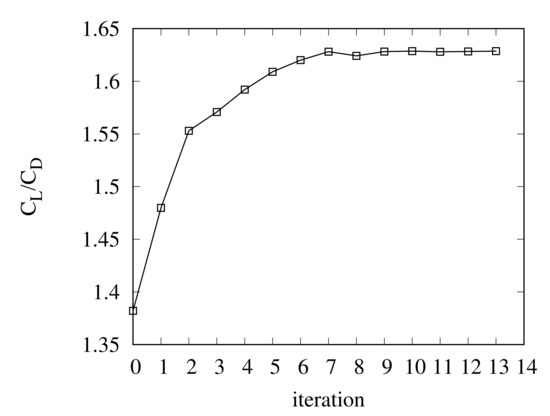
Figure 8.
Iteration history of time-averaged lift-to-drag ratio .
Table 2.
Change in time-averaged lift-to-drag ratio value by shape optimization procedure.
4. Results and Discussion
All calculations were computed on an NEC SX-8R supercomputer of Cybermedia Center, Osaka University. The validations of our numerical solvers for the flow-through two-dimensional corrugated airfoil at a fixed angle of attack or the angle of attack passively changed by the fluid force were conducted in our previous article [28]. All numerical calculations are conducted enough times until the flow fields were fully developed and the aerodynamic coefficients exhibit adequate convergence. All results are collected by time-averaging.
4.1. Effect of Waves
The improvement in aerodynamic performance for a series of wavy airfoil profiles generated by modifying the number of waves and the width of the ridge and valley in the chord direction is explored in this section. The Reynolds number and the angle of attack applied for this investigation is 1000 and ranges from to with the increments of , respectively. The details of the computational parameters are shown in of Table 1.
Performances and flow characteristics of various wavy airfoil profiles are showed. For comparison, the performances and flow characteristics for the original corrugated and NACA2408 airfoil profiles are listed as well. The aerodynamic performance and profile of the various airfoil geometries are summarized in Table 3 for the angle of attack of . Figure 9, Figure 10, Figure 11, Figure 12, Figure 13 and Figure 14 correspondingly show the flow characteristics such as distribution of mean pressure isolines around the various geometries at the angle of attack of . Cases are labeled as for the explored wavy airfoil profiles, where x varies from 1 to 4. Waves are mainly placed on the different regions of the airfoil, such as on the front part with respect to the case , on the rear part with respect to the case . The width of the ridge and valley in the chord direction and the number of waves are varied, such as the small ridge and valley and many waves for the case , the large ridge and valley and few waves for the case . All of the wavy airfoil shapes and the original corrugated airfoil profile not only have a higher lift but also lower drag compared to the NACA2408 airfoil profile, which is the same as conclusions of several investigations of the corrugated dragonfly wings [18,21,22,23,24,25,26]. Interestingly, in comparison with the original corrugated airfoil profile, and have more distinct waves and show a lower aerodynamic performance (in terms of lift-to-drag ratio) and and have less distinct waves and show higher aerodynamic performance. In particular, has the maximum waves and shows the lowest aerodynamic performance, has the minimum waves and shows the highest aerodynamic performance. For the drag, from the original corrugated airfoil profile to the all wavy airfoil shapes, even if the corrugations and waves on the airfoil are different and changed, there is almost nothing changed, i.e., the value at about except . Thus, the lift coefficient greatly affects the aerodynamic performance compared to the drag coefficient for wavy airfoil shapes.
Table 3.
The time-averaged aerodynamic coefficients and its breakdown for the pressure and friction stress contributions of the various geometries at and . The superscripts p and f denote the pressure and friction stress components, respectively.
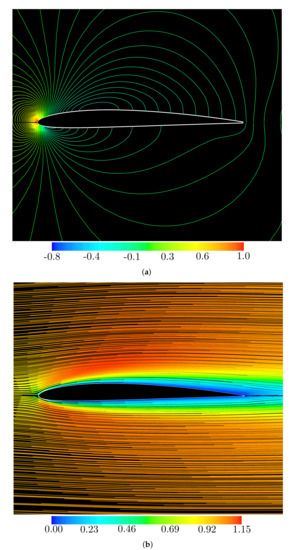
Figure 9.
Flow past the NACA2408 airfoil (Table 3) at and : (a) time-aberaged pressure isolines; and (b) time-averaged steamlines.
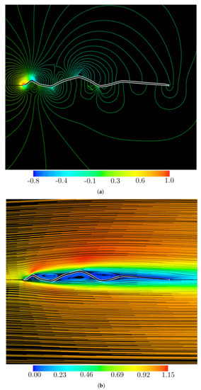
Figure 10.
Flow past the based corrugated airfoil (Table 3) at Re = 103 and α = 0°: (a) time-averaged pressure isolines; and (b) time-averaged streamlines.
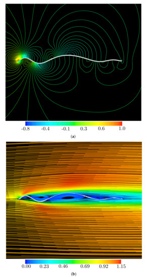
Figure 11.
Flow past the shape Wavy_1 (Table 3) at Re = 103 and α = 0°: (a) time-averaged pressure isolines; and (b) time-averaged streamlines.
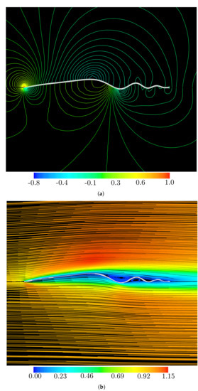
Figure 12.
Flow past the shape Wavy_2 (Table 3) at Re = 103 and α = 0°: (a) time-averaged pressure isolines; and (b) time-averaged streamlines.
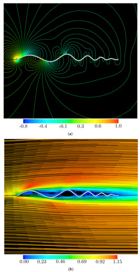
Figure 13.
Flow past the shape Wavy_3 (Table 3) at Re = 103 and α = 0°: (a) time-averaged pressure isolines; and (b) time-averaged streamlines.
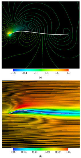
Figure 14.
Flow past the shape Wavy_4 (Table 3) at Re = 103 and α = 0°: (a) time-averaged pressure isolines; and (b) time-averaged streamlines.
Table 3 also shows the breakdown of lift and drag coefficients for the contributions of the pressure and friction stress in various geometries. The superscripts p and f denote pressure and friction stress contributions, respectively. For instance, the pressure stress contribution of the lift is represented as . It can be seen that the breakdown components of the lift coefficient with the different wavy airfoil shapes are almost the same, while the breakdown components of the drag coefficient concerning the different wavy airfoil shapes is different. The first, for the lift coefficient, the pressure stress component concerning all wavy airfoil shapes, the original corrugated and NACA2408 airfoil profiles are significantly dominant, whereas the frictional components are extremely minor. Through investigations of the pressure distribution of the wavy airfoils in Figure 11a, Figure 12a, Figure 13a, and Figure 14a, It can be confirmed that the negative pressure generated at the valleys of the corrugated airfoil contributes to the increased lift. This also corresponds to the large flow acceleration on the blade upper surface in the streamline distribution, as can be seen in Figure 11b, Figure 12b, Figure 13b, and Figure 14b. Secondly, for the drag coefficient, the pressure stress component accounts for about for , , and the original corrugated airfoil, while the frictional component accounts for about for , and , and the NACA2408 airfoil. That is, and have more distinct waves and are akin to appear as a corrugated airfoil for the drag, see Figure 9, Figure 11 and Figure 13. However, and have less distinct waves and are akin to appear as a smoothed surface NACA2408 airfoil for the drag, see Figure 10, Figure 12 and Figure 14. From Figure 11a and Figure 13a, we seem to confirm that the reason why the pressure stress component of the drag coefficient for the wavy airfoils ( and ) is dominant is that the downstream side and upstream side are low pressure and high pressure, respectively. On the other hand, the reason why the frictional stress component of drag for the wavy airfoils ( and ) is large is that large airfoil surface areas face the external flow, see Figure 12a and Figure 14b. In Figure 11b and Figure 13b, it can be seen that there is a distinct trapped vortex in each cavity of the wavy airfoil which causes the main external flow to pass the airfoils without facing the surface area of the airfoil. However, compared to the streamlines around and airfoils, the large surface area faces the external flow for and airfoil
In order to discuss the effect of the angle of attack significantly on the aerodynamic performance (in terms of lift-to-drag ratio) with respect to various airfoil geometries, Figure 15 shows the aerodynamic performance of various wavy airfoil shapes, the original corrugated and NACA2408 airfoil profiles at as the angle of attack is varied from to . Above all, we could confirm that the angle of attacks has almost no effect on the aerodynamic performance of various geometries, apart from a small region of negative angle of attacks for and . Therefore, it is completely acceptable that antecedent computations are performed at an angle of attack to evaluate the influence of airfoil geometries on the aerodynamic performance. From the results of Figure 15 and Table 3, we can confirm that the geometry shape of exhibits the highest aerodynamic performance. Thus, in order to obtain as much as possible the highest global aerodynamic performance wavy airfoil shape, the subsequent aerodynamic optimization procedure begins with the highest aerodynamic performance airfoil shape as the initial geometry.
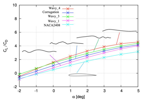
Figure 15.
Flow past various geometries at : variation with angle of attack of time-averaged lift-to-drag ratio.
4.2. Shape Optimization
After an investigation of the effect of waves on an airfoil with the envelope of NACA2408 airfoil, we carry out shape optimization for high aerodynamic performance (in terms of time-averaged lift-to-drag ratio) using a continuous adjoint method. The airfoil is selected as the initial profile guess for aerodynamic shape optimization in order to obtain as much as possible the highest global aerodynamic efficiency wavy airfoil shape. The Reynolds number is and the angle of attack is . Table 4 presents the aerodynamic performance and profile of the optimal airfoil obtained applying our optimization procedure for the aerodynamic efficiency maximization. For comparison, the data for the initial geometry and the original corrugated airfoil are also listed. It can be found that, from Table 4, the shape of the optimal airfoil is similar to a curved plate wing without waves on the airfoil even though the initial guess has waves on the airfoil. Compared to the initial geometry and the corrugated airfoil, the optimal airfoil is associated with higher aerodynamic efficiency, as well as higher lift coefficient. The optimal airfoil shape corresponds to an increase of over the aerodynamic efficiency (lift-to-drag ratio) from the initial geometry, an increase of concerning the corrugated airfoil. The corresponding increase in lift is with respect to the initial geometry and with respect to the corrugated airfoil. However, in comparison with the initial airfoil geometry, only a very little improvement of the drag for the optimal airfoil appears.
Table 4.
Mean aerodynamic coefficients and its breakdown for the pressure and friction stress components of the initial airfoil geometry and optimal airfoil for aerodynamic efficiency maximization at and .
Figure 16 shows the distribution of pressure isolines and streamlines for the flow past the optimal airfoil shape. Here, for each color of the streamline and pressure isolines, the threshold values are the same as those in Figure 9, Figure 10, Figure 11, Figure 12, Figure 13 and Figure 14 for the color bar. From the results in Table 4, the breakdown of the lift coefficient for the optimal airfoil is dominated by the pressure component, while the breakdown of the drag coefficient is dominated by the frictional contribution. These reasons can be found from the distribution of pressure isolines and streamlines in Figure 16. The optimal airfoil is similar to a curved plate and represents the upward convex. The acceleration of the flow near the upper surface of the optimal airfoil is therefore remarkable, it is considered that the pressure distribution on the upper surface of the blade is reduced and the lift coefficient is greatly earned. Since the optimal airfoil does not have distinct corrugations on the airfoil, there is no trapped vortex in each cavity of the corrugations which limits the surface of the airfoil directly facing the external flow. From this point of view, it can be seen that the shape of the airfoil obtained by optimizing the wavy airfoil model does not have the aerodynamic characteristics of a corrugated airfoil but have the aerodynamic characteristics of a smoothed-face airfoil.
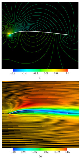
Figure 16.
Flow past the optimal airfoil (Table 4) at Re = 103 and α = 0°: (a) time-averaged pressure isolines; and (b) time-averaged streamlines.
4.3. Hydrodynamic Moment and Attitude Stability
Using the airfoil shape obtained by the shape optimization for the aerodynamic efficiency maximization performed above, numerical calculations related to hydrodynamic moment of force and attitude stability are conducted. The details of this computation are described in our previous article [28].
4.3.1. For the Problem Setting of Fixed Angle of Attack
First, for the problem setting of a fixed angle of attack, the moment coefficient because of the fluid force for the optimal airfoil is evaluated, in which the support point is at chord length from the airfoil leading edge. The time-averaged data of the static moment coefficient are collected after the value exhibits adequate convergence. The mean static moment coefficient of the optimal airfoil at with varying angle of attack is showed in Figure 17, where with increment of . We know that, if an airfoil is stable in the range of , as increases the hydrodynamic moment of force for the airfoil should increase as well, moreover, the direction of the increase of the hydrodynamic moment of force should be the opposite to the direction of increase of . In Figure 17, it can be seen that the slope of the moment coefficient of the fluid force concerning the angle of attack is negative in the range of , i.e., the angle of attack in this region is statically unstable for the optimal airfoil.
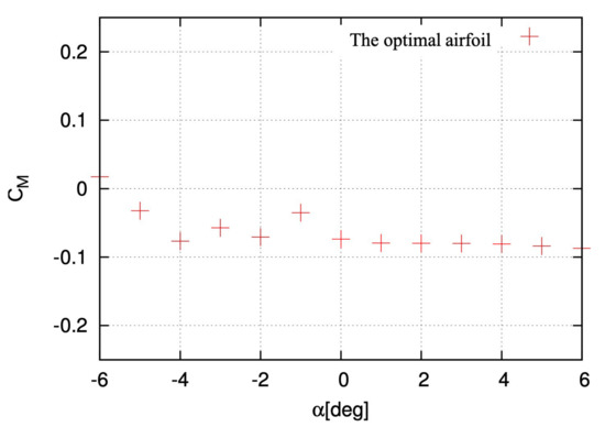
Figure 17.
The mean static moment coefficient of the optimal airfoil at with varying angle of attack.
Figure 18 shows the distribution of the lift coefficient with respect to dimensionless time at Reynolds number 4000, the angle of attack . After the dimensionless time , the evolution of the lift coefficient becomes quasi-stationary, but it can be seen that it oscillates periodically. In Figure 19, the distribution of vorticity around the optimal airfoil at and , and dimensionless time is showed. From Figure 19, it can be seen that vortices are periodically discharged from the leading edge of the optimal airfoil, which may indicate the reason why the lift coefficient oscillates greatly and periodically. After further computation, it has been confirmed that the vortex shedding at the optimal airfoil leading edge is in the range of the angle of attack . Actually, the range of having the vortex shedding exactly corresponds with the range of the angle of attack with the hydrodynamic moment fluctuating. Based on the above discussion, as a conclusion, the optimal airfoil is either statically unstable or statically quasi-stable.
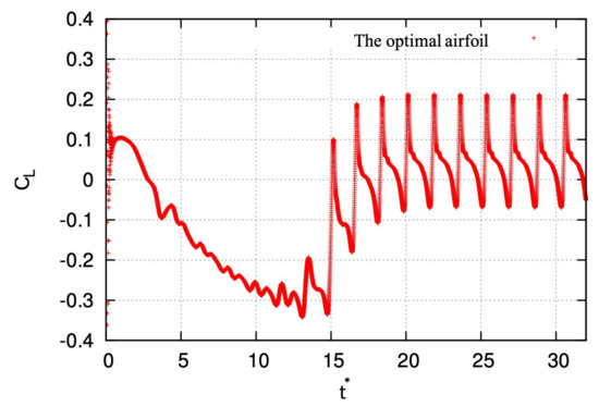
Figure 18.
Time evolution of lift coefficient for the optimal airfoil at and .
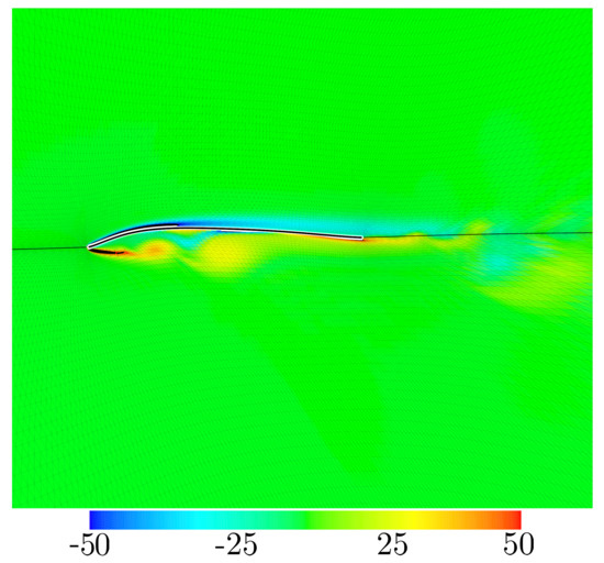
Figure 19.
Distribution of vorticity around the optimal airfoil at , , and dimensionless time .
4.3.2. For the Problem Setting of Angle of Attack Passively Changed by the Fluid Force
In order to balance the initial hydrodynamic moment of force because of the fluid force acting on the airfoil at an initial , a constant moment of force is used, where the rotating support point is at chord length from the leading edge and the initial is at . We observe the time evolution of the objective airfoil’s after an initial disturbance, i.e., , is imposed. More details of the computational setup are introduced in our previous article [28]. Figure 20 shows the time evolution of for the optimal airfoil, the original corrugated and NACA2408 airfoil at with the initial . From this figure, the time evolution of the angle of attack for the corrugated and NACA2408 airfoil is relatively stable and its amplitude is increasingly large. For the optimal airfoil, the angle of attack keeps the initial angle of attack with an initial disturbance, which indicates it is neutral with respect to the moment of fluid force. However, as the dimensionless time pass, the angle of attack increases quickly and diverges in a positive direction. From the above results, coupled with the distribution of the moment coefficient of the fluid force concerning the fixed angle of attack in Figure 17, it can be confirmed that the optimal airfoil is destabilized.
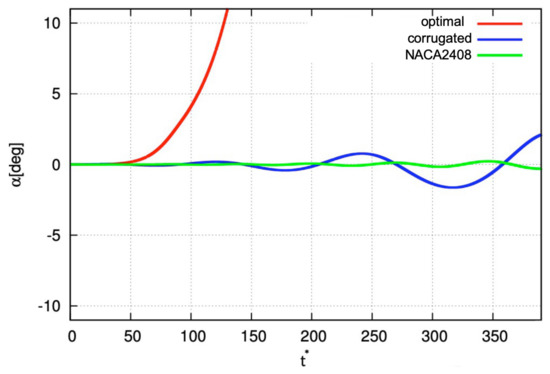
Figure 20.
Time evolution of angle of attack at with the initial .
5. Conclusions
In this study, the effect of the number of waves and the width of the ridge and valley in chord direction for a wavy airfoil was investigated at the angle of attack of and Reynolds number of . All these wavy airfoil geometries have a higher lift, as well as, lower drag in comparison with that of NACA2408 airfoil profile. Interestingly, compared to the original corrugated airfoil profile, the wavy airfoils that have more distinct waves show a lower aerodynamic performance (in terms of lift-to-drag ratio) and the wavy airfoils that have less distinct waves show higher aerodynamic performance. In particular, the wavy airfoil that has the maximum waves shows the lowest aerodynamic performance and the wavy airfoil that has the minimum waves shows the highest aerodynamic performance. For the breakdown of the lift and drag coefficient concerning the pressure and friction stress contributions, the pressure stress contributions are significantly dominant for all wavy airfoil shapes concerning the lift, whereas the drag coefficient concerning the different wavy airfoil shapes are different, such as the pressure stress component accounts for about for the wavy airfoils that have more distinct waves, while the frictional stress component accounts for about for the wavy airfoils that have less distinct waves. From the distribution of pressure isoline and streamlines around wavy airfoils, it is confirmed that the pressure stress contribution of the drag are dominant due to high pressure on the upstream side and low pressure on the downside; the frictional stress contribution of the drag is dominant because of the large surface area facing the external flow. An adjoint-based aerodynamic shape optimization method was utilized to find as much as possible the highest global aerodynamic efficiency wavy airfoil shape at Reynolds number and angle of attack . Interestingly again, the shape of the optimal airfoil is similar to a curved plate without distinct waves on the airfoil even though the initial guess has waves on the airfoil. The optimal airfoil shape corresponds to an increase of over the aerodynamic efficiency from the initial geometry and increase of concerning the original corrugated airfoil. The corresponding increase in lift is concerning the initial geometry and concerning the original corrugated airfoil. The optimal airfoil has an approximate drag coefficient compared to the initial geometry and the original corrugated airfoil. The hydrodynamic moment of force and attitude stability of the optimal airfoil was investigated as well. Concerning an fixed angle of attack, the optimal airfoil is statically unstable in the range of the angle of attack from to , statically quasi-stable from to , where the vortex is shedding at the optimal airfoil leading edge. Concerning an angle of attack passively varied due to the fluid force, the optimal airfoil keeps the initial angle of attack value with an initial disturbance, then quickly increases the angle of attack and diverges in the positive direction. From the above, it is confirmed that the optimal airfoil is destabilized.
Author Contributions
H.T. and Y.L. (Yulong Lei) conceived the original ideal; H.T. wrote and edited the manuscript; and Y.L. (Yulong Lei), X.L., K.G., and Y.L. (Yanli Li) supervised the study. All authors have read and agreed to the published version of the manuscript.
Funding
This research was funded by the project of the Chinese National Natural Science Foundation (Grant No. 51575220).
Acknowledgments
The authors thank Takeo Kajishima for their help with the numerical method.
Conflicts of Interest
The authors declare no conflict of interest.
Abbreviations
The following abbreviations are used in this manuscript:
| MAVs | micro-air vehicles |
| NAVs | nano-air vehicles |
| PAVs | pico-air vehicles |
| SOR | successive over-relaxation |
| UAVs | unmanned aerial vehicles |
References
- Pines, D.J.; Bohorquez, F. Challenges facing future micro-air-vehicle development. J. Aircr. 2006, 43, 290–305. [Google Scholar] [CrossRef]
- Petricca, L.; Ohlckers, P.; Grinde, C. Micro-and nano-air vehicles: State of the art. Int. J. Aerosp. Eng. 2011, 2011, 214549. [Google Scholar] [CrossRef]
- Wood, R.J.; Finio, B.; Karpelson, M.; Ma, K.; Perez-Arancibia, N.O.; Sreetharan, P.S.; Tanaka, H.; Whitney, J.P. Progress on ‘pico’air vehicles. Int. J. Robot. Res. 2012, 31, 1292–1302. [Google Scholar] [CrossRef]
- Pelletier, A.; Mueller, T.J. Low Reynolds number aerodynamics of low-aspect-ratio, thin/flat/cambered-plate wings. J. Aircr. 2000, 37, 825–832. [Google Scholar] [CrossRef]
- Shyy, W.; Lian, Y.; Tang, J.; Viieru, D.; Liu, H. Aerodynamics of Low Reynolds Number Flyers; Cambridge University Press: Cambridge, UK, 2007; Volume 22. [Google Scholar]
- Ukken, M.G.; Sivapragasam, M. Aerodynamic shape optimization of airfoils at ultra-low Reynolds numbers. Sadhana 2019, 44, 130. [Google Scholar] [CrossRef]
- Carmichael, B.H. Low Reynolds Number Airfoil Survey, Volume 1; NASA Technical Report: Capistrano Beach, CA, USA, 1981.
- Lissaman, P.B.S. Low-Reynolds-number airfoils. Annu. Rev. Fluid Mech. 1983, 15, 223–239. [Google Scholar] [CrossRef]
- Mueller, T.J.; DeLaurier, J.D. Aerodynamics of small vehicles. Annu. Rev. Fluid Mech. 2003, 35, 89–111. [Google Scholar] [CrossRef]
- Thom, A.; Swart, P. The forces on an aerofoil at very low speeds. Aeronaut. J. 1940, 44, 761–770. [Google Scholar] [CrossRef]
- Sunada, S.; Yasuda, T.; Yasuda, K.; Kawachi, K. Comparison of wing characteristics at an ultralow Reynolds number. J. Aircr. 2002, 39, 331–338. [Google Scholar] [CrossRef]
- Kunz, P.J.; Kroo, I. Analysis and design of airfoils for use at ultra-low Reynolds numbers. Fixed Flapping Wing Aerodyn. Micro Air Veh. Appl. 2001, 195, 35–59. [Google Scholar]
- Mateescu, D.; Abdo, M. Analysis of flows past airfoils at very low Reynolds numbers. Proc. Inst. Mech. Eng. Part G J. Aerosp. Eng. 2010, 224, 757–775. [Google Scholar] [CrossRef]
- Takizawa, K.; Henicke, B.; Puntel, A.; Kostov, N.; Tezduyar, T.E. Space-time techniques for computational aerodynamics modeling of flapping wings of an actual locust. Comput. Mech. 2012, 50, 743–760. [Google Scholar] [CrossRef]
- Takizawa, K.; Tezduyar, T.E.; Kostov, N. Sequentially-coupled space–time FSI analysis of bio-inspired flapping-wing aerodynamics of an MAV. Comput. Mech. 2014, 54, 213–233. [Google Scholar] [CrossRef]
- Takizawa, K.; Tezduyar, T.E.; Buscher, A. Space–time computational analysis of MAV flapping-wing aerodynamics with wing clapping. Comput. Mech. 2015, 55, 1131–1141. [Google Scholar] [CrossRef]
- Wakeling, J.M.; Ellington, C.P. Dragonfly flight. I. Gliding flight and steady-state aerodynamic forces. J. Exp. Biol. 1997, 200, 543–556. [Google Scholar]
- Kesel, A.B. Aerodynamic characteristics of dragonfly wing sections compared with technical aerofoils. J. Exp. Biol. 2000, 203, 3125–3135. [Google Scholar]
- Sane, S.P. The aerodynamics of insect flight. J. Exp. Biol. 2003, 206, 4191–4208. [Google Scholar] [CrossRef]
- Rees, C.J. Form and function in corrugated insect wings. Nature 1975, 256, 200–203. [Google Scholar] [CrossRef]
- Khan, M.D.; Padhy, C.; Nandish, M.; Rita, K. Computational Analysis of Bio-Inspired Corrugated Airfoil with Varying Corrugation Angle. J. Aeonaut. Aerosp. Eng. 2018, 7, 1000208. [Google Scholar] [CrossRef]
- Luo, G.; Sun, M. The effects of corrugation and wing planform on the aerodynamic force production of sweeping model insect wings. Acta Mech. Sin. 2005, 21, 531–541. [Google Scholar] [CrossRef]
- Rudolph, R. Aerodynamic properties of Libellula quadrimaculata L.(Anisoptera: Libellulidae), and the flow around smooth and corrugated wing section models during gliding flight. Odonatologica 1978, 7, 49–58. [Google Scholar]
- Vargas, A.; Mittal, R.; Dong, H. A computational study of the aerodynamic performance of a dragonfly wing section in gliding flight. Bioinspir. Biomim. 2008, 3, 026004. [Google Scholar] [CrossRef] [PubMed]
- Okamoto, M.; Yasuda, K.; Azuma, A. Aerodynamic characteristics of the wings and body of a dragonfly. J. Exp. Biol. 1996, 199, 281–294. [Google Scholar] [PubMed]
- Murphy, J.T.; Hu, H. An experimental study of a bio-inspired corrugated airfoil for micro air vehicle applications. Exp. Fluids 2010, 49, 531–546. [Google Scholar] [CrossRef]
- Obata, A.; Sinohara, S. Flow visualization study of the aerodynamics of modeled dragonfly wings. AIAA J. 2009, 47, 3043–3046. [Google Scholar] [CrossRef]
- Tang, H.; Lei, Y.; Li, X.; Fu, Y. Numerical Investigation of the Aerodynamic Characteristics and Attitude Stability of a Bio-Inspired Corrugated Airfoil for MAV or UAV Applications. Energies 2019, 12, 4021. [Google Scholar] [CrossRef]
- Hu, H.; Tamai, M. Bioinspired corrugated airfoil at low Reynolds numbers. J. Aircr. 2008, 45, 2068–2077. [Google Scholar] [CrossRef]
- Du, G.; Sun, M. Aerodynamic effects of corrugation and deformation in flapping wings of hovering hoverflies. J. Theor. Biol. 2012, 300, 19–28. [Google Scholar] [CrossRef]
- Sun, W.H.; Miao, J.M.; Tai, C.H.; Hung, C.C. Optimization Approach on Flapping Aerodynamic Characteristics of Corrugated Airfoil. Int. J. Aerosp. Mech. Eng. 2011, 5, 364–371. [Google Scholar]
- Quagliarella, D.; Della Cioppa, A. Genetic algorithms applied to the aerodynamic design of transonic airfoils. J. Aircr. 1995, 32, 889–891. [Google Scholar] [CrossRef]
- Pierret, S.; Van den Braembussche, R.A. Turbomachinery blade design using a Navier–Stokes solver and artificial neural network. ASME J. Turbomach. 1999, 121, 322–326. [Google Scholar] [CrossRef]
- Ahn, C.S.; Kim, K.Y. Aerodynamic design optimization of a compressor rotor with Navier–Stokes analysis. Proc. Inst. Mech. Eng. Part A J. Power Energy 2003, 217, 179–183. [Google Scholar] [CrossRef]
- Jones, D.R.; Schonlau, M.; Welch, W.J. Efficient global optimization of expensive black-box functions. J. Glob. Optim. 1998, 13, 455–492. [Google Scholar] [CrossRef]
- Pironneau, O. On optimum profiles in Stokes flow. J. Fluid Mech. 1973, 59, 117–128. [Google Scholar] [CrossRef]
- Pironneau, O. On optimum design in fluid mechanics. J. Fluid Mech. 1974, 64, 97–110. [Google Scholar] [CrossRef]
- Giles, M.B.; Pierce, N.A. An introduction to the adjoint approach to design. Flow Turbul. Combust. 2000, 65, 393–415. [Google Scholar] [CrossRef]
- Mohammadi, B.; Pironneau, O. Shape optimization in fluid mechanics. Annu. Rev. Fluid Mech. 2004, 36, 255–279. [Google Scholar] [CrossRef]
- Okumura, H.; Kawahara, M. Shape optimization of body located in incompressible Navier–Stokes flow based on optimal control theory. Comput. Model. Eng. Sci. 2000, 1, 71–77. [Google Scholar]
- Reuther, J.; Jameson, A.; Farmer, J.; Martinelli, L.; Saunders, D. Aerodynamic shape optimization of complex aircraft configurations via an adjoint formulation. In Proceedings of the 34th Aerospace Sciences Meeting and Exhibit, Reno, NV, USA, 15–18 January 1996. [Google Scholar]
- Nadarajah, S.K.; Kim, S.; Jameson, A.; Alonso, J.J. Sonic boom reduction using an adjoint method for supersonic transport aircraft configurations. In IUTAM Symposium Transsonicum IV; Springer: Dordrecht, The Netherlands, 2003; pp. 355–362. [Google Scholar]
- Soto, O.; Lohner, R.; Yang, C. An adjoint-based design methodology for CFD problems. Int. J. Numer. Methods Heat Fluid Flow 2004, 14, 734–759. [Google Scholar] [CrossRef]
- Abraham, F.; Behr, M.; Heinkenschloss, M. Shape optimization in steady blood flow: A numerical study of non-Newtonian effects. Comput. Methods Biomech. Biomed. Eng. 2005, 8, 127–137. [Google Scholar] [CrossRef]
- Anderson, W.K.; Venkatakrishnan, V. Aerodynamic design optimization on unstructured grids with a continuous adjoint formulation. Comput. Fluids 1999, 28, 443–480. [Google Scholar] [CrossRef]
- Mohammadi, B. Optimization of aerodynamic and acoustic performances of supersonic civil transports. Int. J. Numer. Methods Heat Fluid Flow 2004, 14, 893–909. [Google Scholar] [CrossRef]
- Jain, S.; Bhatt, V.D.; Mittal, S. Shape optimization of corrugated airfoils. Comput. Mech. 2015, 56, 917–930. [Google Scholar] [CrossRef]
- Naka, H.; Hashimoto, H. Effects of passive deformation of dragonfly wings on aerodynamic characteristics. Trans. Jpn. Soc. Mech. Eng. 2016, 82, 15–21. [Google Scholar]
- Naka, H.; Hashimoto, H. Effect of flapping motion and feathering motion on dragonfly’s flight. J. Jpn. Soc. Des. Eng. 2016, 51, 788–801. [Google Scholar]
- Ciarlet, P.G. The Finite Element Method for Elliptic Problems; SIAM Publication: University City, PA, USA, 2002; Volume 40. [Google Scholar]
- Kajishima, T.; Taira, K. Computational Fluid Dynamics; Springer: New York, NY, USA, 2017. [Google Scholar]
- Tezduyar, T.; Behr, M.; Mittal, S.; Johnson, A. Computation of unsteady incompressible flows with the stabilized finite element methods: Space-time formulations, iterative strategies and massively parallel implementations. ASME Press Vessel. Pip. Div. Publ. PVP 1992, 246, 7–24. [Google Scholar]
- Tezduyar, T.; Aliabadi, S.; Behr, M.; Johnson, A.; Mittal, S. Parallel finite-element computation of 3D flows. Computer 1993, 26, 27–36. [Google Scholar] [CrossRef]
- Johnson, A.; Tezduyar, T. Mesh update strategies in parallel finite element computations of flow problems with moving boundaries and interfaces. Comput. Methods Appl. Mech. Eng. 1994, 119, 73–94. [Google Scholar] [CrossRef]
- Thompson, J.F.; Soni, B.K.; Weatherill, N.P. Handbook of Grid Generation; CRC Press: Boca Raton, FL, USA; New York, NY, USA; Washington, DC, USA; London, UK, 1998. [Google Scholar]
- Chorin, A.J. A numerical method for solving incompressible viscous flow problems. J. Comput. Phys. 1967, 2, 12–26. [Google Scholar] [CrossRef]
- Tamura, A.; Kikuchi, K.; Takahashi, T. Residual cutting method for elliptic boundary value problems. J. Comput. Phys. 1997, 137, 247–264. [Google Scholar] [CrossRef]
- Kajishima, T.; Ohta, T.; Okazaki, K.; Miyake, Y. High-order finite-difference method for incompressible flows using collocated grid system. JSME Int. J. Ser. B Fluids Therm. Eng. 1998, 41, 830–839. [Google Scholar] [CrossRef]
- Tang, H.; Lei, Y.; Li, X.; Fu, Y. Large-Eddy Simulation of an Asymmetric Plane Diffuser: Comparison of Different Subgrid Scale Models. Symmetry 2019, 11, 1337. [Google Scholar] [CrossRef]
- Tang, H.; Lei, Y.; Fu, Y. Noise Reduction Mechanisms of an Airfoil with Trailing Edge Serrations at Low Mach Number. Appl. Sci. 2019, 9, 3784. [Google Scholar] [CrossRef]
- Tang, H.; Lei, Y.; Li, X. An Acoustic Source Model for Applications in Low Mach Number Turbulent Flows, Such as a Large-Scale Wind Turbine Blade. Energies 2019, 12, 4596. [Google Scholar] [CrossRef]


© 2020 by the authors. Licensee MDPI, Basel, Switzerland. This article is an open access article distributed under the terms and conditions of the Creative Commons Attribution (CC BY) license (http://creativecommons.org/licenses/by/4.0/).