Article

Influence and Impact of Data Averaging and Temporal Resolution on the Assessment of Energetic, Economic and Technical Issues of Hybrid Photovoltaic-Battery Systems

1
Independent Researcher, 87036 Rende, Italy
2
Department of Mechanical, Energy and Management Engineering, University of Calabria, 87036 Rende, Italy
3
Wroclaw University of Science and Technology, Wyb. Wyspianskiego 27, 50370 Wroclaw, Poland
*
Author to whom correspondence should be addressed.
Energies 2020, 13(2), 354; https://doi.org/10.3390/en13020354
Submission received: 31 October 2019 / Revised: 18 December 2019 / Accepted: 27 December 2019 / Published: 10 January 2020
(This article belongs to the Collection Smart Grid)

Abstract

:
The temporal resolution of the demand and generation profiles may have a significant impact on the estimation of self-sufficiency and self-consumption for consumers and prosumers. As an example, measuring the load profile, with a low temporal resolution, may lead to the under-estimation of energy consumption, while measuring solar irradiation with a low temporal resolution may lead to the over-estimation of on-site energy generation. Storage systems may reduce errors due to the lower temporal resolution by 8–10 times or even more, depending on the capacity of the batteries. Besides self-generation and self-consumption, there are other indicators that can be influenced by temporal resolution that deserve to be investigated. This is a detailed study of the influence of temporal resolution and the time averaging on a hybrid photovoltaic-battery system; this study encompasses both economic and technical aspects, from the calculation of savings on the electricity bill to the estimation of the equivalent cycles of battery storage system. To this end, the three-minute load profile of a real case study is used to obtain other three load profiles with temporal resolution equal to 15, 30, and 60 min via data averaging. Therefore, the authors analyze the influence and the impact of temporal resolution and data averaging in terms of: The size of the photovoltaic generator and the capacity of the storage system; the savings in the electricity bill and the balance between costs and savings; the peak values and the average values of power flows during high generation and low generation; the profile of the storage system over the year; the utilization rate of the storage system and the rated power of the electronic converter that regulates the charge and the discharge; the profile of the state of charge of the storage system and the life-time estimation of batteries through the calculation of the equivalent number of cycles.

1. Introduction

Besides the reduction of technology costs, the government support via economic and fiscal incentives are key factors for the diffusion of systems with renewable energy sources. In the period 2005–2014, these systems benefited from the subsidies of 135 billion dollars worldwide; at the end of 2017, subsidies have increased from 135 to 143 billion dollars with an average growth rate of 2% per year. In 2014, the governments of Germany, United States of America, and Italy paid half of the worldwide subsidies. In 2017, this scenario changed because China was the main supplier of subsidies to renewables, ahead of Germany, United States, Japan, and Italy; together, these five countries account for almost 65% of total renewable energy subsidies. Today China, United States, Brazil, Germany, and India are the five countries that, in decreasing order, have the greatest capacity to generate energy from renewable sources; China is the leader, both in terms of photovoltaic capacity and wind capacity, as shown in Table 1. On the other hand, if the population of these countries as in Table 2 is considered, Germany and Denmark achieve the leadership for capacity per capita for photovoltaic (PV) and wind (WG), respectively; the small Ireland is the runner-up in per capita wind capacity [1,2].
Historically, wind farms and photovoltaic plants received most of the subsidies; in 2017 they obtained more than 80% of the total support and represent 70% of the global non-hydroelectric renewable energy production. In 2017, roughly 52 GW of wind turbines were installed so the worldwide installed capacity is about 539 GW (+11% compared to 2016). In the same year, roughly 98 GW of photovoltaic modules were installed so the worldwide installed capacity is about 402 GW. Bioenergy is the third most supported renewable energy technology in 2017. In the future scenarios, subsidies to renewables will grow further, up to a peak of $300 billion in 2035 (doubling rate in about 16 years), with a decrease to $280 billion in 2040. Wind farms and photovoltaic plants will still have most of the support, that is more than three quarters of the support; bioenergy will receive 15% [1,2,3].
The data summarized above clearly shows that the future of renewables is promising. Although, it remains heavily dependent on government support policies; indeed, this combination of renewable sources and supporting government policies is unstable due to a handful of reasons. First of all, despite the extraordinary growth of photovoltaic and wind power plants in the world, the generation of energy from renewable sources is not keeping up with the rapid growth in energy demand. In 1987, fossil fuels covered 81% of the world’s energy consumption, after thirty years, this percentage has remained unchanged [1,2]. As shown in Figure 1, in 2015 the world total primary energy supply by fuel is still dominated by coal, oil and natural gas. Nuclear has increased over time, as well as biofuels and waste; hydro and others (geothermal, solar, wind, tide/wave/ocean, heat, and others) are last. On the other hand, a different scenario from the one shown in Figure 1 would have been improbable given that, in the last years, for each dollar given as subsidy to renewables, $2.60 have been given to fossil fuels. In addition, the energy generated from renewable sources and the energy demand are not shared between the consumption sectors in the same proportions. Notwithstanding the difficulties related to development for renewables, Chinese policy makers and planners are integrating the demand and supply of distinct sectors—electrifying heating, manufacturing, and transport—in those parts of the country where there is a large penetration of renewable energy generation [4,5].
On the other hand, as the energy demand is converted into electricity demand, problems of electric transmission lines become more acute. This is because photovoltaic and wind generators produce power in an intermittent way, therefore with increased penetration of renewables, the harder is to satisfy the demand when these generators are not available or are not sufficiently productive. The absence of generation from renewable sources is already a substantial and expensive problem, even when this absence is known in advance; for example, the Californian independent system operator (CAISO) managed the eclipse on 21 Monday 2017, securing a power reserve 3.8 times greater than it normally handles [6]. Two years before, a solar eclipse passed over the Atlantic Ocean and it was visible across Europe; the European transmission system operators published a report about the estimated impact well in advance [7]. Network operators in Germany spent 3.6 million euros to double the usual power reserve; in Italy, 4 GW capacity was prepared [8]. Therefore, it is necessary to create flexibility in this direction, so that the generation and demand find their balance and, at the same time, the electricity grids operate in a safe and economic way.
Storage systems, both centralized and distributed, play an extremely important role in the direction of flexibility, since they contribute to reliability [9] and adequacy [10] of power systems [11], and to the management of the uncertainty of power generation from renewables [12,13,14]. The great improvement in system dynamic performance is already discussed since decades and is provided by the application of a battery energy storage (BES) system to the load frequency control of interconnected power systems [15], to the bus voltage control in three-phases distribution lines [16]; the same applies to battery storage systems, even when installed on electric vehicles, and sustainable energy development of emerging economies [17]. For all this reasons, the dimensioning and positioning in electrical grids, as well as the planning and real-time management of storage systems are deeply investigated issues [18,19,20,21,22]. When decentralized and built using electrochemical batteries, storage systems are notoriously a practical, fast, modular, and cost-effective tool to guarantee residential and commercial end-users a high self-consumption rate, savings on bills and providing higher reliability [23,24,25,26,27,28,29,30,31].
This paper contributes to this area, focusing its attention on a grid-connected hybrid photovoltaic-battery system at residential and commercial level.

1.1. State of the Art

The literature reports show that having data with high temporal resolution can be a mandatory issue in order to reach correct and precise conclusions. For example, Richardson et al. in [32] present an energy demand model to be used as a tool in the design of the local distribution network. The model returns the profile of the household load—the aggregated load profile—starting from the profiles of single appliances, previously created synthetically. Each synthetic profile faithfully reproduces the real-use case, since the temporal resolution is 1 min. The volatility of the demand for each single home, minute-by-minute, as well as the power factor of the aggregated load are almost perfectly represented in the 100–1000 W range; the energy consumption for powers up to 10 W, and above 1000 W are under-estimated as the night-time demand is under-estimated, mainly because the model does not exactly represent people’s behaviour (English men and women in the case of the paper) who leave the lights on while they sleep.
The close correlation between the electricity demand and the habits of the occupants of a dwelling is a central node for Richardson and for Widen et al. in [33]; the Markov-chain model, presented by Widen, reproduces a high resolution numerical series, stochastically generated, which represent the profile of a family’s demand; these series are useful for evaluating the performance of small scale energy systems and indoor building climate. To generate the numerical series, the Widen’s model first synthetically generates activities for each family member using 1-min real data, and then it calculates the aggregated profile of members.
Marszal et al. in [34] propose a high-resolution load model to facilitate the modeling of flexible energy buildings. Like Richardson, Marszal uses a bottom-up approach so the use of a single appliance is the basic brick to create synthetic data in order to obtain the one-minute profile of a typical Danish family. The comparison of the synthetic data with the measured data shows that the Marszal’s model captures well all the characteristics of the families’ profiles; the sole exception is the under-estimation of energy consumption for powers over 1000 W and the under-estimation of electricity demand during spring and summer, mainly due to the fact that the model under-estimates the need for lighting in these periods.
Wright et al. in [35] measure the load profile of eight houses for each minute and evaluate the effect of time-averaging from 1 min to 5, 15, and 30 min on the statistics of both the on-site generation and load profiles. The analysis shows that as the measurement recording interval increases, the load peaks reduce or disappear completely; high-frequency cyclic loads, such as heating appliances are no longer evident if the temporal resolution is greater than 1 min. Wright also reports that time intervals longer than 1 or 2 min have a significant effect on all basic statistical surveys, except on the calculation of the average: Maximum and highest percentile values are reduced, the median increases. Wright also adds that five-minute data averaging is a reasonable compromise for the evaluation of on-site generation with good precision; 30-min data averaging can still provide a reasonable estimation of the energy generated on-site and the energy exported to the local grid, but it is not for the estimation of the imported energy.
For Huld et al. in [36], the on-site generation is given by a photovoltaic thin film cells; the efficiency of such a generator is estimated as a function of the temporal resolution of the local irradiance and temperature. Huld shows that monthly-average data lead to an over-estimation of efficiency of about 2%; this is not a great error if compared to the uncertainty in the measurement of solar irradiance but it can be equally significant because it is a systematic error, therefore, it can negatively affect the estimation processes, such that it is carried out by the web application of the Photovoltaic Geographical Information System (PVGIS) of the European Commission. For Widen et al. in [37] the on-site generator is a conventional photovoltaic module; the researchers discuss the massive integration in low-voltage power grids of the distributed generation and the possible negative impacts due to the excess of power generation on the grid, taking into account the time averaging from 10 min to 60 min and a simplified model of a real 0.4 kV low-voltage distribution grid in Uppsala, Sweden. Widen concludes that time averaging negatively impacts the statistical properties of the load demand in individual households, whereas, this impact is almost null for both the on-site generation and the aggregated load profile (the latter is already smoothed by random coincidence).
Talavera et al. in [38] propose a new approach based on cost-competitiveness to size the photovoltaic generator and maximize self-consumption. In this sense, the researchers measured the energy consumption of three houses located in South of Spain for an entire year with one-minute time intervals; they also performed a quality check by removing the invalid measurements and processing the remaining data according to the recommendations of the IEC 61724 standard. Talavera concludes that the adopted temporal resolution let to the conclusion that the daily, monthly, and annual self-consumption rates are between 0.5 and 0.6. Therefore, half of the load demand can be met through self-consumption, without local storage.
Also Ayala et al. in [39] considers that conventional photovoltaic modules and studies how the self-consumption rate and the self-sufficiency rate changes with the increase in the temporal resolution. Given a 2.3 kW photovoltaic generator is placed on the rooftop and sized in order to reach the zero-energy-building target, Ayala concludes that the self-consumption and self-sufficiency are overestimated by 9% when a temporal resolution of 60 min is used in place of a temporal resolution of 10 seconds.
Cao et al. in [40] calculate a greater error in the averaging effect on both the on-site electrical generation and demand; given that a 183.3 square meter area is entirely covered by photovoltaic modules, such an error increases from 0.2% to 69% when the temporal resolution changes from 5 to 60 min. The coarse resolution causes a large error especially when the generation profile frequently intersects with long and intermittent peaks of the demand profile. Cao concludes that there is no unambiguous indication about the value of the coarser resolution, which should be adopted to obtain results close to those with a one-min resolution, given that the most essential factors are the specific characteristics of the generation and demand profiles. Moreover, Cao extends the study and considers battery storage systems; these systems have a significant effect on the errors reported above, which are reduced 8–10 times because the storage systems hardly level the long, intermittent peaks of the demand profile.
Also Beck et al. in [41] provide an evaluation of the influence of the temporal resolution of both the demand and the on-site generation profiles on self-consumption and on the size of hybrid photovoltaic-battery systems. Given the load profile of a typical family in Germany, and a photovoltaic generator is sized to minimize the electricity bill, Beck affirms that a 15-min generation profile is a good profile in general. As for the demand profile, a 15-min temporal resolution is also a reasonable value on condition that the demand profile does not show the most of the energy consumption for powers above 2 kW, otherwise a 1-min resolution is required for reliable results. Beck also states that, when adopting a storage system, the temporal resolution becomes almost negligible due to the flexibility introduced by the batteries, and indeed, if the demand profile shows frequent peaks and a large quantity of energy is consumed for powers above 2 kW then a temporal resolution of 5 min leads to errors lower than 5% in estimating the self-consumption rate; temporal resolutions up to 60 min may still be acceptable, depending on specific characteristics of the load profile.
A hybrid photovoltaic-battery system and the temporal resolution of input data are also the two pillars of the study presented by Wolf et al. in [42]. The electrical load consumption, solar radiation, and the indoor temperature of a real case were measured every 15 seconds; these data were used to calculate further profiles with different temporal resolution. Wolf concludes that, in the absence of a storage system, a 1-min temporal resolution is necessary in order to limit the error on self-consumption to 5%. In the presence of a storage system, such an upper limit is also achieved in the case of 60-min temporal resolution or even longer depending on the size of the battery. In fact, the results obtained by Wolf need further investigation as the numerical experiments carried out do not take into account the power of the storage system, that is, the charge and discharge power of the battery system have no limits.
A more complete hybrid system is studied by Hoevenaars et al. in [43]; indeed, besides a photovoltaic generator and batteries, the researchers also considered variable residential loads, wind power generation, and a diesel genset. The influence of temporal resolution was first studied for each component, one at time. Hoevenaars states that the energy produced by the wind turbine increases up to a maximum of 7% as the temporal resolution varies from 1 second to 1 hour, whereas, the fuel consumption of the genset reduces to a maximum of 5.6%. Hoevenaars also states that the operation of both, the photovoltaic generator and the batteries are not affected by the length of the time step. Subsequently, the influence of temporal resolution was studied for the optimization of the entire system; the obtained results return that the impact of the temporal resolution depends on the configuration of the hybrid system and, in particular, on the type of backup source, i.e., the batteries and the genset. Hoevenaars concludes that the temporal resolution has higher impact when the genset is operating, and that it is not possible to determine the optimal temporal resolution without having performed a simulation of the given entire system.

1.2. The Contribution of this Paper

The contributions from the literature show that the temporal resolution of the demand and generation profiles may have a significant impact on the estimation of self-sufficiency and self-consumption for consumers and prosumers. As an example, load profiles that are measured with a temporal resolution greater than 1 min, may lead to the under-estimation of energy consumption and the inability to identify electrical loads. The low temporal resolution can also determine an over-estimation of the energy output of a photovoltaic generator installed on the rooftop in a very wide range, from 9% to 69%. Self-consumption is also overestimated by 9% if the temporal resolution is greater than 10 seconds. All these errors are strongly reduced, 8–10 times, by storage systems. On the other hand, these contributions do not consider the influence of temporal resolution on common issues of great interest to consumers, such as the savings on the electricity bills or the influence on technical issues, such as the power flows in the hybrid system and the utilization rate of the storage system.
This paper provides a detailed study of a hybrid photovoltaic-battery system, which evaluates the influence of the data averaging and the temporal resolution on energetic issues, such as self-generating and self-consumption. In addition, this paper extends the previous studies to cover technical and economic issues, such as the sizing of the hybrid system and the life estimation of the batteries. To this end, the three-minute load profile of a real case is considered; via data averaging, further three load profiles with temporal resolution equal to 15, 30, and 60 min are obtained. Therefore, the authors analyse the influence and the impact of temporal resolution and data averaging in terms of: the size of the photovoltaic generator and the capacity of the storage system, the savings on the electricity bill and the balance between costs and savings, the peak values and the average values of power flows during low generation and high generation, the profile of the storage system over the year and during four particular months, the utilization rate of the storage system and the rated power of the electronic converter that regulates the charge and the discharge of storage system, the profile of the state of charge and the life-time estimation of the batteries through the calculation of the equivalent number of cycles.

2. The Hybrid Photovoltaic-Battery System

The scheme of a typical grid-connected hybrid photovoltaic-battery system, suitable for residential and commercial applications, is depicted in Figure 2a; the photovoltaic generator, the storage system, the aggregated load, and the meter are shown along with their respective profiles: PPV, PLOAD, PBES, and PGRID. For the latter, it is appropriate to distinguish between the power flow from the system to the grid, Pexported, and power flow to the system, Pimported; such a distinction is necessary for the calculation of the electricity bill, the net-metering, etc. In practice, the realization of a hybrid photovoltaic-battery system requires, first selecting the system configuration, by choosing between the two system configurations illustrated in Figure 2b,c. The configuration in Figure 2b is typical for new installations where both the generator and the storage are brand new and installed at the same time. The power converter A is a dc-dc converter that ensures the tracking of the maximum power point of the photovoltaic generator, the power converter B is a current-controlled dc-ac converter that injects an AC current that, in most of applications, is in phase with the voltage detected at the output terminals. The power converter C is a dc-dc converter which regulates both the charge and discharge of the batteries. It is a step-up or step-down type, depending on preferences and choices during design, including the number of cells of batteries that realize the storage system. All these power electronic converters, A, B and C, are interconnected with each other by means of a centralized controller, which acquires information and measurements in order to optimize the operation of the hybrid system as a whole. The small number of converters makes the use of a single microcontroller possible for executing all the measurements and calculations, including the generation of pulse-width modulation signals for the switches of all the converters. The configuration, illustrated in Figure 2c, refers to the so-called retrofit of an existing system, where the photovoltaic generator has already been installed on the rooftop, before and, in a second step, a new storage system is installed. When retrofitting, the power electronic converters A, B, and C rarely communicate or cooperate with each other, they are not coordinated by a central controller. Sharing a voltage or current measurement can be very difficult, even when these converters adopt an international communication standard, such as the IEC61850.
The configuration of Figure 2d is less known and less widespread than the previous two configurations. It is more expensive but also advantageous in case of a weak distribution grid, when the hybrid system is often forced to operate in islanded mode [44]. Supposing a blackout or an excessive deviation of the amplitude or frequency of the voltage at the point of common coupling, the relay that connects the hybrid system to the grid opens; the converter D’ performs a seamless transition from grid-connected to islanded mode as to ensure in the local grid of the hybrid system a stable voltage, close to the reference values [45,46]. When islanded, the current-controlled converter, B, continues to operate without interruption as the converter D’ compensates for over generation and under generation. Since a failure of the converter B determines the disconnection of the unique power generator inside the hybrid system and the total collapse of the system itself, the additional converter C’ provides a solution; it increases the cost of the hybrid system, as well as the robustness, since it allows the storage system to be recharged by the photovoltaic generator and, in turn, offers the load to be supplied by the batteries. The two converters C’ and D’ do not necessarily have the same rated power.
As for the operation of the hybrid photovoltaic-battery system, the authors in this paper assumed that the power produced by the photovoltaic generator feeds the electrical loads at first; the remaining power, if any, recharges the batteries in compliance with the rated power of the dc-dc converter and the state of charge. The power flow between the batteries and the utility grid is not allowed: The grid does not recharge the batteries, and therefore, it is not possible to buy and store energy during off-peak hours and consume it during peak hours. The authors also assume that the energy imported from the utility grid is paid at market price, the exported energy to the grid does not imply any income, no incentives or subsides are paid, and net-metering is not considered. Moreover, demand response programs and ancillary services are beyond the scope of this paper. In the next Section 2.1 and Section 2.2, the photovoltaic generator and the battery storage system models are presented; the model of the hybrid photovoltaic-battery system follows in Section 2.3.

2.1. The Model of the Photovoltaic Generator

In the model of the photovoltaic generator adopted in this paper; the average value of the power generated by the photovoltaic generator PPV(∆t) in the time interval ∆t is a function of the peak power PV of the generator, of the solar radiation G(∆t) and of two parameters as follows:
PPV(∆t) = PV∗G(∆t)·η1·η2
The parameter η1 in (1) is defined as:
η1 = 1 − 0.4982%·(Tmod(∆t) − TSTC)
and takes into account the difference between the operating temperature of the photovoltaic module and the standard test temperature. This is because the peak power of the photovoltaic module is certified in standard operating conditions and the test temperature TSTC is set to 25 °C; therefore, the authors assume a variation of the actual power with respect to the peak one equal to 0.4982% for each Centigrade degree of difference between the module temperature and the test temperature.
The temperature of the module Tmod in (1) is defined as:
Tmod(∆t) = Tamb(∆t) + α·G(∆t)
That is, as the sum of the ambient temperature Tamb(∆t) and the product between the parameter α and the solar radiation G(∆t). The parameter α is 0.035 °C/(W/m2) for a ground-mounted system or 0.050 °C/(W/m2) for a building-integrated system. The parameter η2 in (1) takes into account the power losses, due to the tilt shading and local shading, the power losses due to reflection and mismatching, and the power losses in DC and AC circuits and inverters.

2.2. The Model of the Battery Energy Storage System

The model of the battery storage system adopted in this paper mainly includes the capacity of the batteries set, the nominal power PBES of the batteries set, the state of charge SOC(∆t) and the power flow PBES(∆t) of the batteries; other parameters, such as the batteries voltage and current, are omitted. During the discharge of the batteries, the power exported by the batteries is upper limited to the nominal power:
PBES (∆t) ≤ PBES.
Power flows higher than PBES are never allowed, also in very short intervals. During the recharge of the batteries, the power imported by the batteries is upper limited to the nominal power multiplied by the coefficient m:
PBES (∆t) ≤ m·PBES.
The value of the coefficient m can be set greater or lower than 1, to simulate a fast or a slow recharge. In this paper, the value of m is set to 1. As the power flow varies, the state of charge of the storage system varies accordingly from a previous value SOC(h−1) to a new one SOC(h),
SOC(h) = SOC(h−1) + (PBES(∆t)·∆t/BES)·(1/ηd)·100
SOC(h) = SOC(h−1) + (PBES(∆t)·∆t/BES)·ηc·100
where ηd and ηc account for the efficiency during the discharge, and the recharge, respectively. The self-discharge phenomenon has been considered negligible.

2.3. The Model of the Hybrid Photovoltaic-Battery System

This paragraph describes the model of the hybrid photovoltaic-battery (PV&BES) system of Figure 1. In order to size the hybrid photovoltaic-battery system, a typical objective function is also provided. Given the index h = 1…T for the time interval ∆t, the main inputs of the model are the solar radiation G(h), the load demand PLOAD(h), the nominal power of the storage system PBES; the main outputs of the model are the size of the photovoltaic system PV and the capacity of the storage system BES.
maximize (Savings − Costs)
subject to,
h = 1, 2, … T
PPV (h) = PV·G(h)·η1·η2
IF PPV (h) ≥ PLOAD (h)
PBES (h) ≤ PPV(h) − PLOAD(h)
PBES(h) ≤ m·PBES
SOC(h) = SOC(h−1) + (PBES(h)·∆t/BES)·ηcharge·100
IF PPV (h) < PLOAD (h)
PBES (h) > PPV(h) − PLOAD(h)
PBES(h) ≤ PBES
SOC(h) = SOC(h−1) + (PBES(h)·∆t/BES)·(1/ηdischarge)·100
PGRID(h) = PPV(h) − PLOAD(h) − PBES(h)
IF PGRID(h) < 0
Pexported(h) = PGRID(h)
IF PGRID(h) > 0
Pimported(h) = PGRID(h)
k = 1 T P P V ( h ) · Δ t = 100 % k = 1 T P LOAD ( h ) · Δ t
k = 1 T ( P P V ( h ) P exported ( h ) ) · Δ t = 70 % k = 1 T P P V ( h ) · Δ t
Electr . Bill = k = 1 T P imported ( h ) · Δ t · Price ( k )
Savings = Electr.billw/out PV&BES − Electr.billwith PV&BES
Installment (PV) = f(Loan_rate; Loan_lenght; Amount (PV))
Installment (BES) = f(Loan_rate; Loan_lenght; Amount (BES))
Costs= Installment (PV) + Installment (BES)
Balance = Savings − Costs
SOCmin ≤ SOC ≤ SOCmax
PV ≥ 0; BES ≥ 0
The functions and constraints will be discussed in the order as they are numbered. As in Equation (8), the objective function maximizes the difference between savings on bills and costs. Equation (9) sets k as the index over the T time intervals ∆t. Equation (10) calculates the power PPV (h) produced by the photovoltaic generator as the product of the rated power PV, the solar irradiance G (h) and the two parameters η1 and η2 which take into account the ambient temperature, and the combined power system losses, respectively. Equation (11) compares the power of the photovoltaic generator with the load demand; when the generation exceeds the demand, an over-generation exists and batteries can be recharged. Therefore, Equation (12) upper limits the power flow of batteries PBES(h) to the over-generation whereas Equation (13) further upper limits PBES (h) to the rated power PBES multiplied by the coefficient m which, if greater or lower than 1, can be used to accelerate or decelerate the recharge. Finally, Equation (14) updates the state of charge; the new value is the previous value plus a quantity, which depends on the power PBES (h), the storage capacity BES and the parameter ηcharge. Equation (15) compares again the power of the photovoltaic generator with the load demand; if the renewable generation does not exceed the demand, an under-generation exists and batteries can be discharged. Equations (16) and (17) upper limit PBES (h), and Equation (18) consequently updates the SOC. Given the value of PBES (h), Equation (19) calculates the power PGRID (h) at the point of connection to the utility grid. If Equation (20) verifies that PGRID (h) is lower than zero then Equation (21) labels this value as imported power; vice versa, if Equation (22) verifies that PGRID (h) is positive then Equation (23) labels this value as exported power. Equation (24) imposes the zero-net-energy target since the energy produced by the photovoltaic generator during the year must equal the energy consumed by loads (i.e., 100% self-sufficiency). Similarly, Equation (25) imposes self-consumption being equal to 70%. The remaining equations, from (26) to (31), return the calculation of values useful for evaluating costs and savings achieved through the adoption of the hybrid photovoltaic-battery system. In particular, Equation (26) calculates the electricity bill, Electr.Bill, using market energy prices, Price(h), to the imported energy. Therefore, Equation (27) calculates the savings as the difference between the bill when calculated in the presence of the photovoltaic-battery system, Electr.billw/outPV&BES, and in the absence, Electr.billwithPV&BES. Equations (28) and (29) return the annual installment for purchase, install and maintain the photovoltaic generator and the storage system, according to the interest rate, Loan_rate, the length of the loan, Loan_length, and the financed amount, Amount (.). Moreover, Equation (30) calculates the total annual cost while Equation (31) calculates the so-called balance between savings and costs. Equations (32) and (33) constrain the value of the state of charge of the storage system, the peak power of the photovoltaic generator and the capacity of the batteries, respectively.

3. Numerical Experiments

This section illustrates the results of numerical experiments with reference to a real case study.

3.1. The Case Study

The case study is a building of the University of Calabria, placed in the South of Italy; the building consists of eight floors, each floor covers an area of 400 square meters, offices, and laboratories are often on the same floor. A set of data, such as the phase voltage and current, solar irradiance and ambient temperature, has been measured for an entire year using a smart meter mod. 3Ph-WiFi by CretaES [47]; input ports of such a meter allow to sample signals in the 0–3.3 V and 0–100 kHz range every 200 µs. The measured values are averaged over longer periods of time. For example, the smart meter has returned the load profile PLOAD in the form of a string of 175,200 positive/negative/null numbers; the temporal resolution is equal to 3 min, hereinafter also referred to as R3. The yearly energy consumption is 121 MWh; interior lighting covers about 30% of annual consumption, the rest is for other electrical loads. The electricity bill is about €11,769. Other data are: The market electricity prices, the market price for photovoltaic generators and for the lithium-ion battery storage system, the interest rate for a bank loan.

3.2. Load Profile, Temporal Resolution and Time Averaging

Given the load profile PLOAD with a three-minute temporal resolution, namely R3 resolution, the authors have calculated three load profiles with different temporal resolution by applying time averaging. The temporal resolutions of these three new profiles are 15 min, 30 min and 60 min, hereinafter also referred to as R15, R30 and R60.
As an example, Figure 3 illustrates the load profile on 1st of July; in particular, Figure 3a illustrates the load profile as it has been returned by the smart meter whereas Figure 3b–d illustrate the time-averaged load profiles.

3.3. Influence on the Size of the Photovoltaic Generator and Capacity of the Battery Energy Storage System

The model of the PV&BES system, shown in Section 2 of this paper, is now used to optimal sizing both the photovoltaic generator and the battery energy storage system; the optimal solution minimizes the cost function, it ensures that the self-generation rate is equal to 100% and the self-consumption rate is 70%. When R3 is considered, the optimal size for the photovoltaic generator is 83.38 kW while the optimal capacity of the batteries storage is 105.17 kWh, as reported in the first column of Table 3. Such a calculation is now repeated with reference to R15, R30 and R60; the remaining columns of Table 3 show that the optimal size of the photovoltaic generator remains unchanged and equals 83.38 kW, while the optimal capacity of the batteries slightly decreases from 105.10 kWh to 103.01 kWh (−1.98%). The conclusion is that the temporal resolution has no particular relevance in the optimal sizing of the PV&BES system, as time averaging from 3 to 60 min does not imply any relevant error; for the case studied, time averaging underestimates the capacity of the batteries storage system by only 2%.
The second half of Table 3 reports the energy EPV produced by the photovoltaic generator during the year, the energy EBES stored by the batteries during the year, the energy EIMP imported from the grid during the year as a function of the temporal resolution; the value of EPV does not vary and remains equal 121.64 MWh, the value of EBES decreases from 30.69 MWh to 29.25 MWh (−4.69%), the value of EIMP increases from 36.49 MWh to 37.93 MWh (+2.84%). These results clearly indicate that the temporal resolution has small influence on the calculation of energies EPV, EBES and EIMP therefore it is easy to deduce that the influence of the temporal resolution on the electricity bill and savings is equally irrelevant. In this respect, the first column of Table 4 shows the electricity bill, when calculated in the absence of both the photovoltaic generator and the storage system, i.e., Billw_outPV&BES, is €11,769.39, where €7501.81 (63.74%) is for the electricity consumption and €4267.58 (36.26%) is for taxes and VAT. Adopting the hybrid PV&BES system, the bill reduces to €3562.33 therefore the saving is about 69.73%. On the other hand, some additional costs exist: The annual installment for the photovoltaic generator is, €15,077.46 and the annual installment for the storage system is €3214.79; therefore, the balance between savings and installments is €−10,085.18. When the temporal resolution varies from 3 min to 60 min, the balance varies by +0.04%. Therefore, the conclusion is that the temporal resolution has no relevance on the calculation of the balance between savings and costs when a hybrid PV&BES system is adopted.

3.4. Influence on Power Flows During an Over Generation

This section discusses the influence of the temporal resolution on peak values of these four profiles: PLOAD, PLOAD − PPV, PBES and PESP; they are the load profile, the difference between the load profile and the photovoltaic generator profile, the profile of the battery storage system, and the profile of the power exported to the utility grid, respectively. As reported in the first column of Table 5, the peak of PLOAD is 52 kW and it significantly decreases to 31.50 kW as the temporal resolution changes from R3 to R60. The conclusion is that a 60-min temporal resolution can cause a substantial under-estimation (39.42%) of the peak value of the load profile; since current peaks are under-estimated too, the estimation of the number of times that the electric cables are overloaded is jeopardized [15].
When negative, the difference PLOAD − PPV indicates that the photovoltaic generator produces more than the load demand; in this case an over generation is in progress and the batteries can be recharged. Worth noting is that PLOAD − PPV is the power available for the recharge and that it does not necessarily coincide with PBES. The peak value of PLOAD − PPV is 77.12 kW for R3 and it decreases to 60.83 kW for R60 (−21.12%), as shown in the second row of Table 4. Similarly, the peak value of PBES is 73.27 kW for R3 and it decreases to 60.83 kW (−24%) for R60, as shown in the third row of Table 3. The peak value of PBES is lower than the peak value of PLOAD − PPV because of two reasons; the first relates to the state of charge. Indeed, if the storage system is fully charged then the over-generated power is necessarily exported to the grid or locally dissipated, penalizing the self-consumption rate. The second relates to the rated power of the electronic converter, which regulates of the battery recharge; if such a rated power is lower than the peak value of PLOAD − PPV than a part of the over-generated power is necessarily exported to the grid or locally dissipated, further penalizing the self-consumption rate. The estimate of the decrease of the self-consumption rate, due to the under-estimation of the rated power of the batteries recharger, requires precise numerical calculations because it depends on how many times, and for how long, the rated power of the recharger is found to be lower than PLOAD − PPV. For example, a battery’s recharge with a rated power equal to 60.83 kW, i.e., the peak value of PLOAD − PPV for R60, instead of 73.27 kW, i.e., the peak value of PLOAD − PPV for R3; the numerical results returns a self-consumption rate still of 70%. The conclusion is that a coarse temporal resolution can induce the under-sizing of the power converter that regulates the recharge of the batteries; in this case, a part of the power generated by the local generators is necessarily exported to the grid or locally dissipated, thus penalizing the self-consumption rate. The estimate of the reduction in the self-consumption rate requires specific calculations, case by case. Lastly, the fourth row of Table 5 shows the peak value of PESP that is the power flow exported to the utility grid; this peak value is 77.02 kW for R3 whereas it is 60.83 kW for R60 resolution (−21%). The conclusion is that the coarse temporal resolution can induce the under-estimation of the feed-in contractual power.

3.5. Influence on Powers During an Under Generation

This paragraph studies the hybrid PV&BES system when PLOAD − PPV is positive, that is the load demand is higher than the on-site generation. In order to compensate for this under generation, the batteries start discharging in compliance with the constraints regarding the state of charge, as well as the rated power of the converter that regulates for the discharge of the batteries themselves. The peak value of PLOAD − PPV is shown in the first row of Table 6. It decreases from 41.35 kW to 25.50 kW (−38.33%) when the temporal resolution changes from 3 min to 60 min. The second row of Table 6 shows the peak value of the power flow of batteries which compensates for the under-generation; the peak value is 32.00 kW for R3 and 24.38 kW for R60 (−23.81%). The conclusion is that a coarse temporal resolution can induce an under-estimation of the rated power of the electronic converter, which regulates the discharge of the storage system, thereby, penalizing the self-consumption rate. In most of the real applications, the batteries’ discharge coincides with the batteries’ recharge. Therefore, the size of such a converter has to be chosen by taking into account the extreme condition between over-generation and under-generation. Finally, if the storage system does not fully compensate for the under-generation then the hybrid PV&BES system imports power from the utility grid. The peak value of PIMP is reported in the last row of Tab 6 and it is 41.35 kW for R3 and 25.50 kW for R60 (−38.33%). The conclusion is that the coarse temporal resolution can induce the under-estimation of the imported contractual power.

3.6. Influence on the Utilization Rate of the Storage System

The influence of the temporal resolution on the calculation of the utilization rate of the storage system is investigated in this paragraph by distinguishing three cases: The storage system is in stand-by mode, recharging, and discharging. The stand-by mode indicates that the batteries storage is functioning, but the output current is zero or almost zero; therefore, the longer the stand-by mode, the lower the utilization rate of the storage system. In order to estimate the utilization rate, PBES provides the necessary information. Indeed, PBES is a string of values whose cardinality depends on the temporal resolution; for example, if the temporal resolution is three minutes then the cardinality of PBES is 175,200 values. The authors assume being null the values belonging to the range of ±0.10 kW. Given this assumption, half of PBES (50.31%) is null when the temporal resolution is 3 min, the utilization rate of the storage system is 49.69%, as reported in the first column of Table 7. The utilization rate increases from 49.69% to 51.29% when the temporal resolution changes from 3 to 60 min. The conclusion is that the poor temporal resolution scarcely influences the estimate of the utilization rate of the storage system.
It is important to underline that the low utilization rate mentioned above is due to the strategy that regulates the operation of the storage system and it is not due to the temporal resolution. Indeed, the adopted strategy means batteries’ recharge occurs exclusively in the presence of an over generation, while the batteries’ discharge occurs exclusively in the presence of under-generation; this strategy excludes any exchange of power between the storage system and the grid.
This strategy clearly limits the use of the storage system and, consequently, the utilization rate. Finally, Table 8 shows the utilization rates when calculated for March, June, September, and December. The utilization rates in March vary with the temporal resolution but they coincide almost exactly with the utilization rates for the whole year. In contrast, the storage system gives a higher contribution to the PV&BES system in June, compared with March; indeed, the rates reported in the third row of Table 8 show higher contribution of about 10%. The utilization rates in September are in the middle between March and June. Finally, December is the month with the lowest utilization rates since the storage system remains inactive for about 60% of time, regardless of the temporal resolution.

3.7. Influence on the Recharge of the Storage System

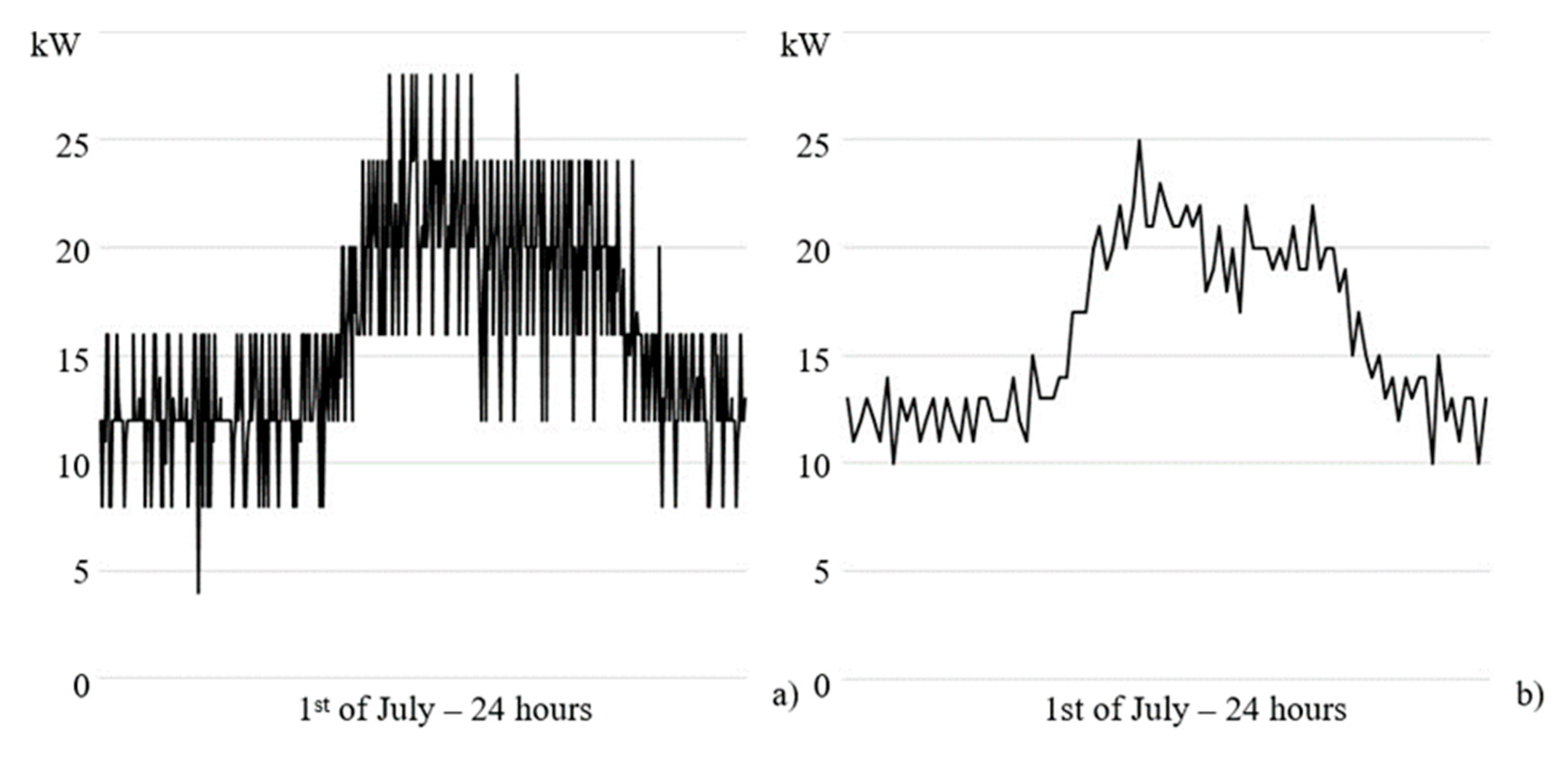
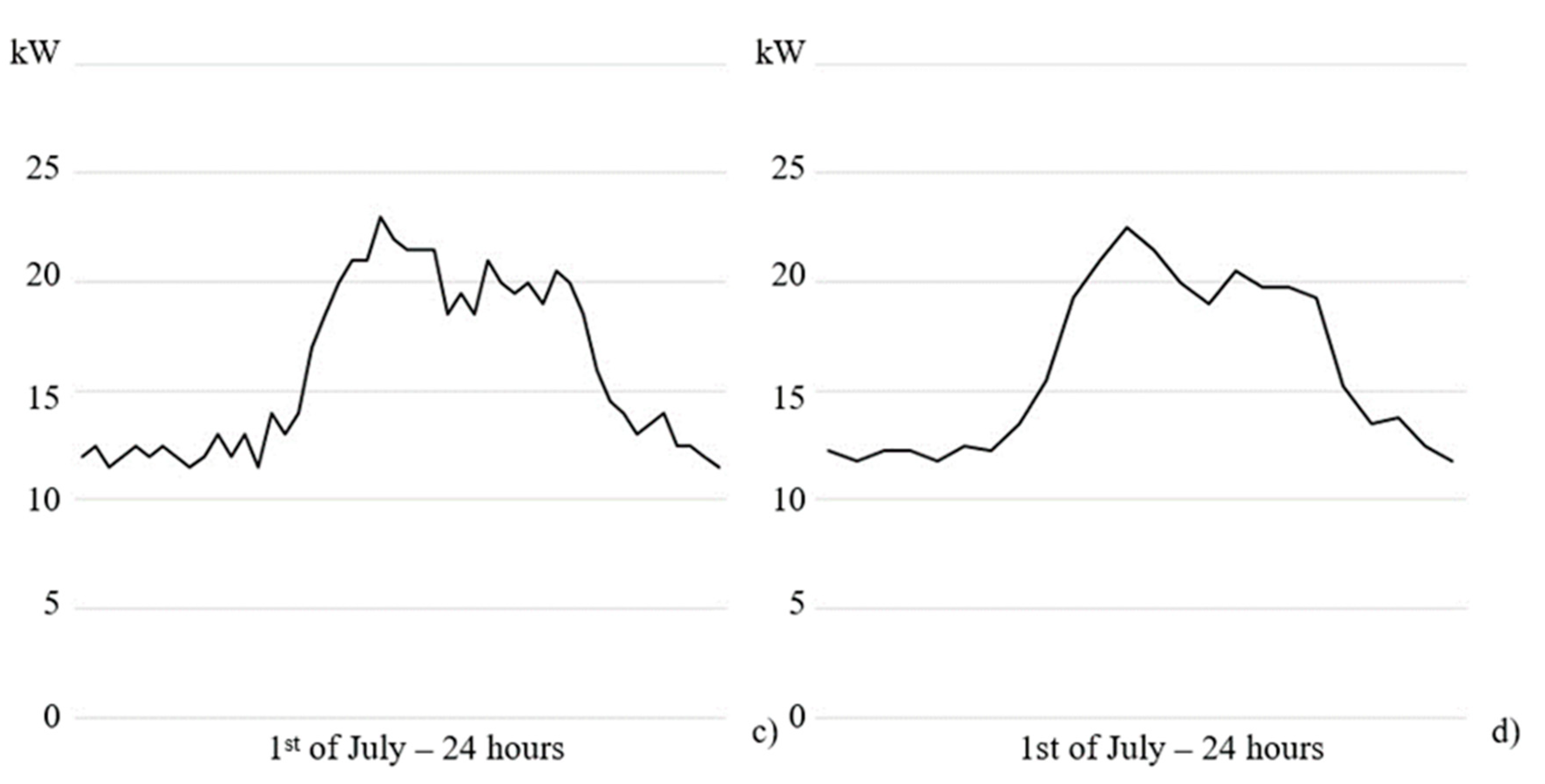
The previous paragraph has studied the profile of the storage system and it has paid attention to null values only, thereby calculating the utilization rate and evaluating the influence of the temporal resolution on it. This paragraph focuses on positive values of PBES, i.e., those values that indicate the batteries recharge. As reported in the third and fourth rows of Table 7, the batteries recharge covers the 17.60% of P
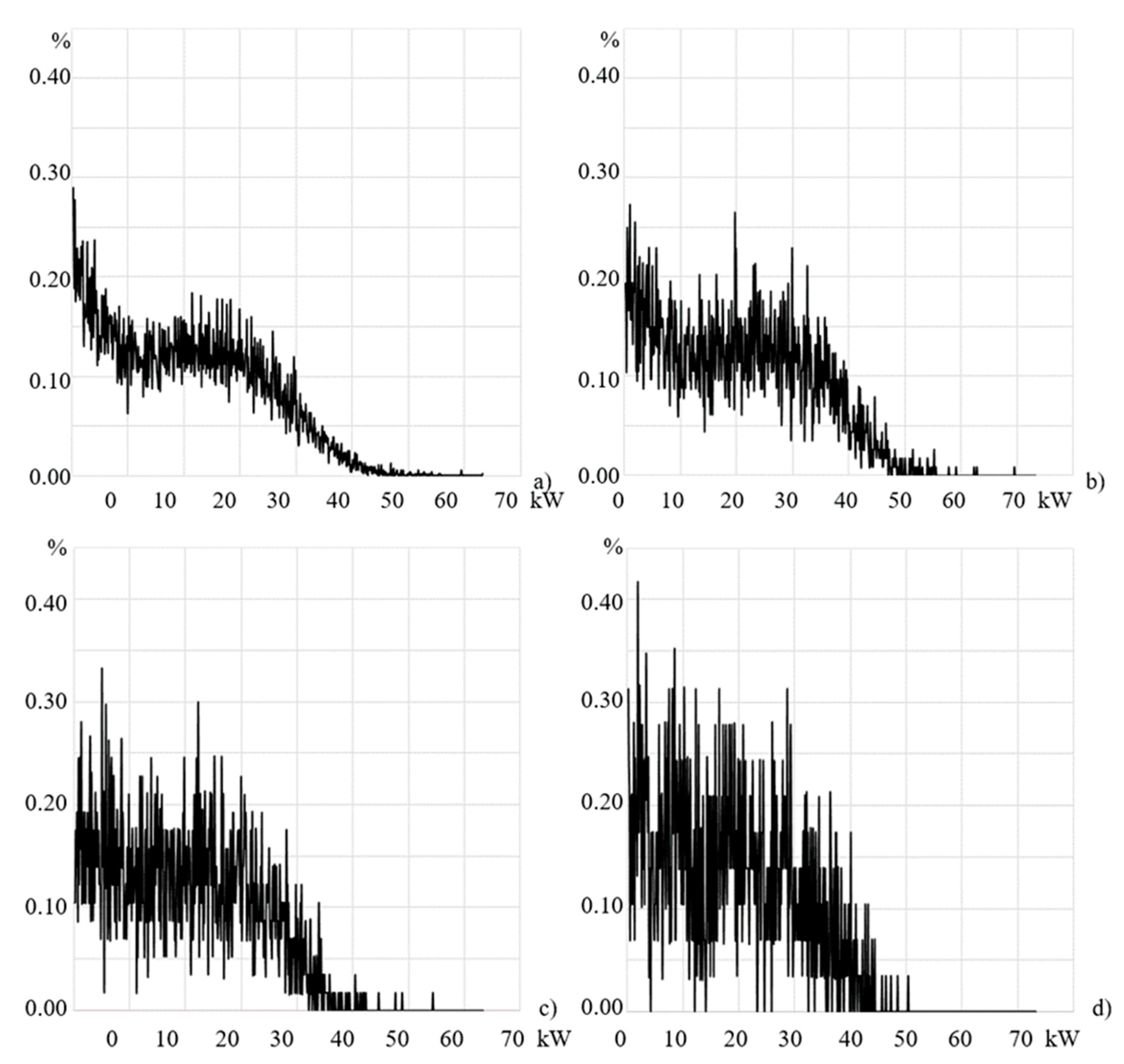
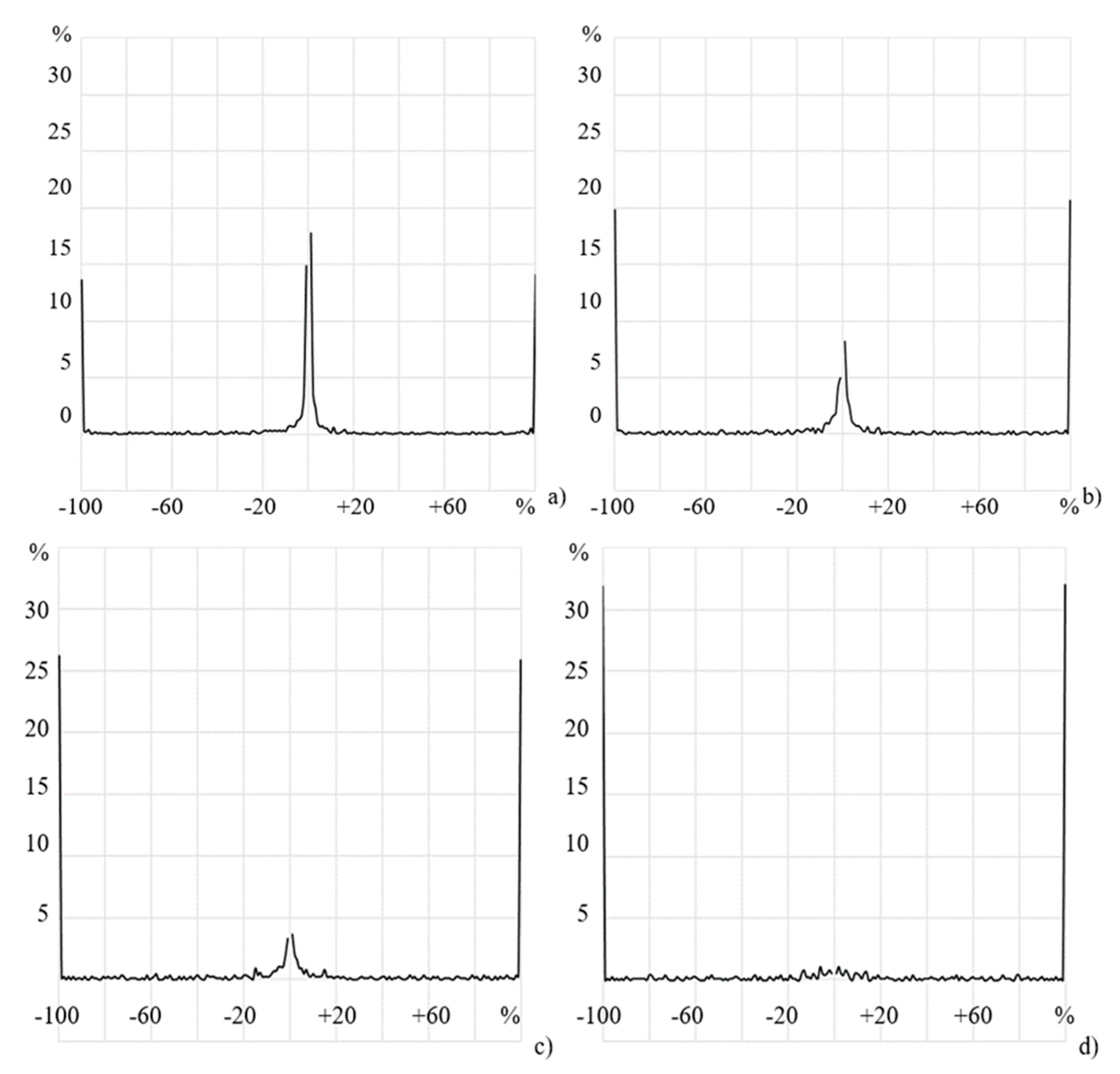
BES and the average value is 19.89 kW when a three-minute temporal resolution is adopted. The authors approximate these values to integers and calculate their recurrences; as an example, the string {5, 7, 9, 9, 9, 5, 5, 5, 5, 5} has ten integers, the number 5 recurs six times or its recurrence is 60%, the recurrence of number 7 is 10%, the number 9 counts for 3 times therefore its recurrence is 30%. This said, Figure 4a illustrates the recurrences of values of the battery storage profile when the temporal resolution is 3 min; in the Figure, 10 kW recurs 0.1% since the number 10 counts in PBES approximately for 176 times. Figure 4a also shows that all values in PBES recur less than 0.3% and that none of the values prevail. Figure 4b–d show the recurrences when the temporal resolution is 15, 30 and 60 min, respectively. A conclusion is: the recurrences of the values belonging to PBES do not vary appreciably when the temporal resolution varies; given a trend line, the dispersion of the values increases as the temporal resolution get worse.
The calculation of the recurrences of PBES in Figure 4 can be a valid aid to sizing the power electronic converter that regulates the batteries; recharge. Indeed, while examining the Figure 4, it can be noted that the values greater than 40 kW recur less than 0.05%, therefore, 40 kW is a valid size of the power converter. In fact, sizing the batteries’ recharger, and taking into account the recurrences of values of PBES, is not sufficient; the corresponding values of energy have to be considered as well. In this regard, Figure 5 associates the values of PBES and the corresponding values of energy stored in the batteries, according to the temporal resolution. Figure 5 shows that all the four curves merge into one and that the energy stored in the batteries for power higher than 40 kW is about 18.56%. Therefore, a 40 kW batteries recharge is no longer a valid choice, since it penalizes self-consumption in a non-negligible way. A 51 kW batteries recharger is more reasonable since, according to Figure 5, it affects the self-consumption by 2.28%. The conclusion is that the temporal resolution does not significantly affect the estimate of the amount of electrical energy stored in the storage system, including the correspondence between the stored energy and the respective values of powers.

3.8. Influence on the Discharge of the Storage System

The two previous paragraphs have studied the profile of the storage system and they have paid attention to positive and null values; this paragraph focuses on the negative values of PBES, which indicate the discharge of the storage system.
When the temporal resolution is 3 min, the discharge of the storage system covers the 32.46% of PBES and the average value of powers during the discharge is 10.78 kW, as in the fifth and sixth rows of Table 7. The authors approximate these negative values of PBES to integers and calculate their recurrences, as already explained and done in the previous paragraph. 
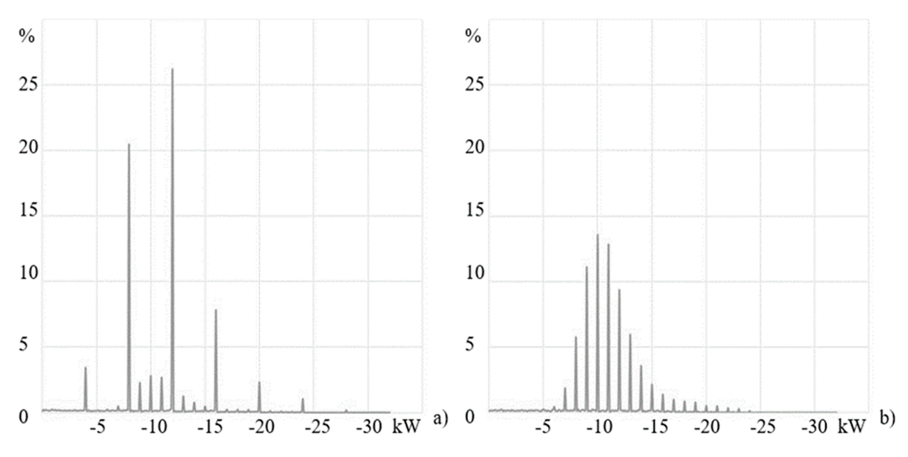
Figure 6a shows the recurrences of values of PBES. Some of these values clearly recur more than others and cause spikes. Recurrences of 12 kW, and 8 kW are 26.24%, and 20.50%, respectively. These two values count almost half of the recurrences. With the exception of 16 kW, which recurs approximately 3%, the remaining values have negligible recurrences. As the temporal resolution get worst, the distribution of recurrences changes and it completely loses spikes. Indeed, the distribution of recurrences for R15, R30 and R60 shown in Figure 6b–d clearly indicates that the more the temporal resolution get worst, the more the discharge of the storage system tends to a unique value, that is 10 kW. The conclusion is that the three-minute temporal resolution allows a set of powers to be identified most frequently exported by the storage system. In other words, the discharge of the storage system takes place in correspondence with a restricted set of power values. The 60-min temporal resolution causes the total loss of this information; the discharge tends to concentrate in the close neighborhood of a single value that, in a high temporal resolution, might count zero times.

3.9. Influence on the State of Charge of Batteries

The previous three paragraphs have studied the influence of the temporal resolution on the utilization rate, the recharge, and the discharge of the storage system. The batteries storage system profile has been the basis of such a study. This paragraph illustrates a similar study but, this time, the basis of the study is the profile of the state of charge (SOC) [
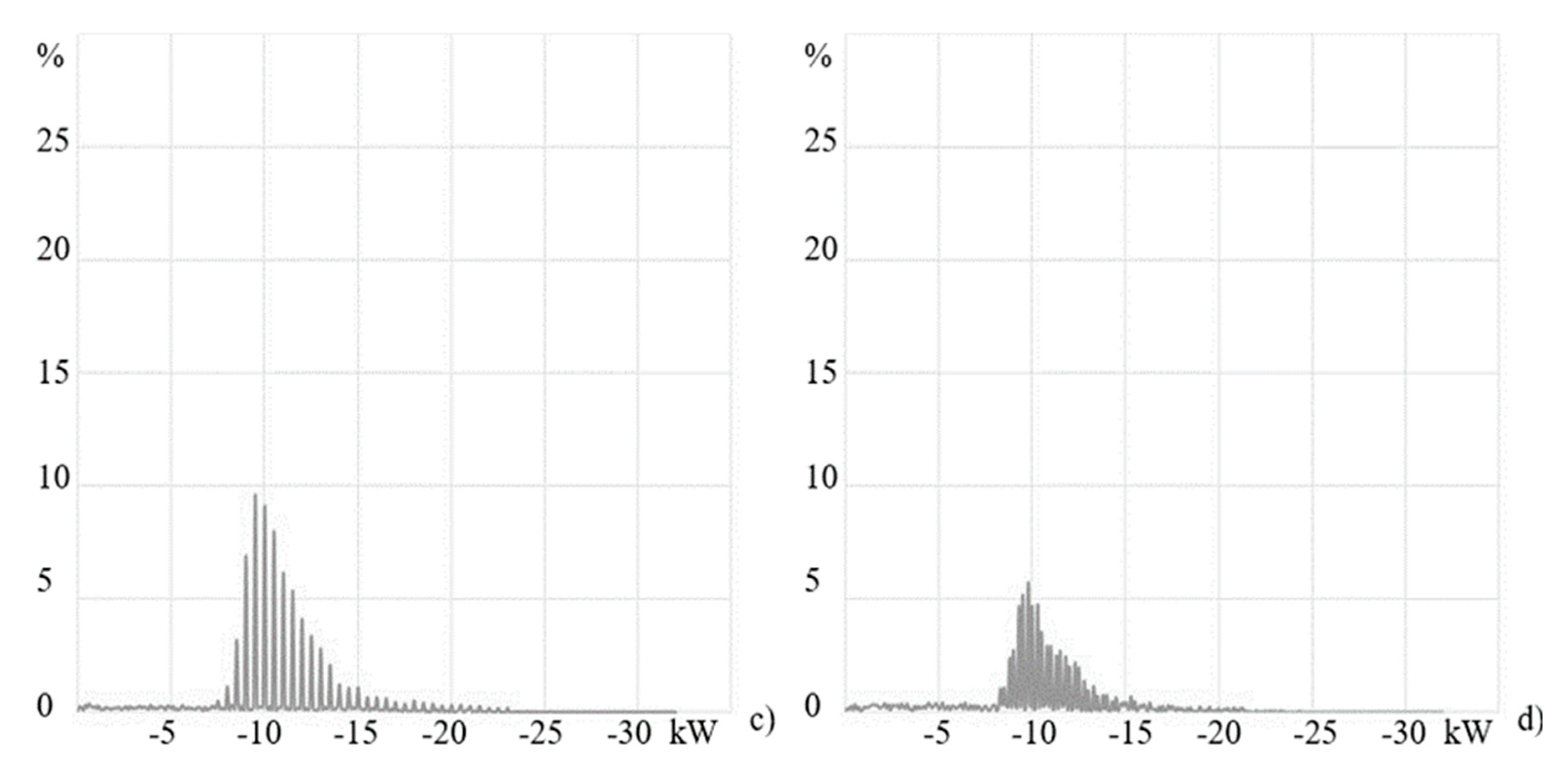
48]. As usual in this field, such a profile is a string of numbers in the range 0–100%; the string length depends on the temporal resolution, it decreases from 175,200 to 8760 values when the temporal resolution changes from 3 to 60 min. The recurrences of SOC’s profile for a three-minute temporal resolution are reported in Figure 7a; this temporal resolution returns a fairly sharp curve where most of the recurrences are equal to about 0.05%. Two spikes are on the range boundaries: If the SOC tends to 0% then the recurrence tends to 4% while if SOC tends to 100%, then the recurrence tends to 2%.
The recurrences of SOC’s profile for a 60-min temporal resolution are reported in Figure 7b; recurrences remain below 1% and no value prevails with respect to the others. The conclusion is that the calculation of recurrences of SOC’s profile is a useful aid in understanding the use of the batteries storage system, but the 60-min temporal resolution compromises the effectiveness of such a calculation as it flattens the distribution of recurrences, forcing them into a restricted range.
The calculation of recurrences of SOC profile is not the solely useful aid in understand the use of the batteries storage system; an alternative exists namely the extraction of the increasing and decreasing substrings from the SOC profile. As an example, the SOC profile is a string of numbers in the range 0–100%; this profile is now divided into M substrings,
SOC = {substring1} & {substring2} & … & {substringM}
where an ascending substring indicates a partial or total recharge whereas a descending substring indicates a partial or total discharge. For sake of simplicity, an ascending substring from 28% to 48% is named sub (+20%) whereas sub (−30%) indicates any descending substring which accounts for a partial discharge of 30%.
This said, the SOC profile in the first ten days of January is divided into M = 240 substrings for a three-minute temporal resolution, or into M = 16 substrings for a 60min temporal resolution. These substrings are shown in Figure 8. The three-minutes temporal resolution allows the true understanding of the use of the batteries. In Figure 8a the storage system executes four 100% recharges, two 75% recharges, one 50% recharge and one 40% recharge; it also executes four 100% discharges, one 75% discharge, two 50% 50% discharges and five discharges within 1–25% range. The 60-min temporal resolution makes the identification of the use of the batteries less precise, indeed in Figure 8b the storage system executes eight discharge/recharge cycles in alternation: Four 100% discharge/recharge, two 75% discharge/recharge, one 50% discharge/recharge and one 40% discharge/recharge. The conclusion is that the 60-min temporal resolution simplifies the use of the storage system, masks both the charges and discharges with small amplitude, and promotes those with a larger amplitude.
The conclusion reported above is the result of a ten-days period of observation, from the 1 to 10 January, It is opportune to verify such a conclusion over a wider period, i.e., the entire year. To this end, Figure 9a shows the recurrences of all substrings of the SOC profile for a 3-min temporal resolution. On the left of Figure 9a, sub (−100%) indicates a full discharge and it recurs 13.63%; on the right of Figure 9a, sub (+100%) indicates a full recharge and it recurs 14.10%. Recurrences of full discharges and full recharges almost coincide each other. Figure 9a also shows that almost all the remaining substrings have negligible recurrences, except for the substrings in the narrow range around zero, i.e., sub (±4%) whose recurrence is about 15–20%. Similarly, Figure 9b–d show the recurrences for temporal resolutions equal to 15, 30 and 60 min, respectively; an evident result is that recurrences of both sub (−100%) and sub (+100%) progressively increase up to about 32%, that is a value two times greater than that measured with a 3-min temporal resolution. Another evident result is that the recurrences of the substrings in the narrow range around zero, i.e., sub (±4%), tends to zero. The conclusion is that dividing the profile of the state of charge of the storage system into substrings and studying these substrings is a valid tool to understand the use of the batteries. The temporal resolution affects the validity of the results from this study, and in particular, the 60-min temporal resolution strongly simplifies the operation of the batteries that tends to an alternation of recharges and discharges of equal amplitude.
Dividing the profile of the state of charge of the storage system into substrings is also a valid tool to estimate the lifetime of the batteries because the recurrences of substrings contributes to estimate the number of equivalent cycles of the storage system. To this end, the second row of Table 9 shows the recurrences of substrings from sub (−100%) to sub (−94%) and from sub (+94%) to sub (+100%); substrings from sub (−93%) to sub (+ 93%) are not considered since they count almost zero. The number of equivalent cycles of the storage system is so estimated:
E F C 1 = i = 94 % 100 % c o u n t ( + s u b i ) + c o u n t ( s u b i ) 2
The number of equivalent cycles EFC1 returned by Equation (35) depends on the temporal resolution; as in Table 9, EFC1 is approximately 232 for a 3-min temporal resolution while it is 242.50 (+4.52%) for a 60-min temporal resolution. The conclusion is that the recurrences of substrings of the SOC profile allows the number of equivalent cycles of the storage system to be calculated which, in turn, allows the lifetime of the batteries to be estimated. Such a calculation is negatively affected by a coarse temporal resolution as the 60-min temporal resolution induce the over-estimation of the number of equivalent cycles by 4.52%.
It is worth pointing out that Equation (35) returns an estimate that is an approximate calculation of the degradation of the storage system. This is because such a formula does not take into account the type of batteries, the operating temperature, the nominal current, or the nominal voltage. Although, all these factors affect the degradation process. Equation (35) can be used in combination to an analogous equation proposed by Berrueta et al. in [49],
E F C 2 = | i | 2 C d t
where |i| is the absolute value of the battery current in amps, where C is the battery capacity in Ah. The number of equivalent cycles EFC2 returned by Equation (36) is reported in the penultimate row of Table 9. It is approximately 247 for the temporal resolution of 3 min, and about 216 (−12.55%) when the temporal resolution is 60 min. The difference between EFC1 and EFC2 is very small; actually it is irrelevant if compared with respect the 4500 cycles of the modern LiFePO4 lithium polymer batteries [50,51]. Although, EFC1 and EFC2 are estimates, they are input data for sophisticated formulas for the batteries aging analysis. As an example, when Wang et al. [52] studied a lithium battery mod. Sanyo UR18650, they grouped the capacity fade and the impedance rise, and thus, obtained the following formula useful to estimate for the decrease of state of health:
S O H = [ 0.0008 · e 0.3903 · | i C | ] · 2 · C · E F C 14876 · t 0.5 · e 24500 R · T
where i is the battery current in amps, C is the battery capacity in Ah, |1/C| is the normalized current, t is the time expressed in days, T is the operating temperature in Kelvin, and R is the gas constant. Equation (37) is the sum of two negative terms where the first is a function of the current, of the capacity and of the equivalent number of cycles, while the second term is a function of the time and the operating temperature. The decrease of state of health returned by Equation (37) is reported in the last row of Table 9; the degradation is 56.09% when calculated with a 3-min temporal resolution, whereas, it is 43.43% when calculated with a 60-min temporal resolution. It is important to note that these values have been calculated using EFC2 and by assuming that the operating temperature remains constant and equal to 20 °C. The latter assumption implies that the second term of Equation (37) is 21.9% per year. The conclusion is that the 60-min temporal resolution causes under-estimation of the degradation of the state of the health by about 13%.

4. Conclusions

This paper presented an in-depth study of the influence of the data averaging and the temporal resolution on a hybrid photovoltaic-battery system. The results were obtained using the real load profile, and covered an entire year with a three-minute temporal resolution, which were then compared with those obtained using a further three profiles with coarser temporal resolution, that is 5, 30, and 60 min.
With respect to the influence on the size of the photovoltaic generator and capacity of the batteries energy storage system, the temporal resolution had no particular relevance in the optimal sizing of the hybrid system in order to guarantee a 100% self-generation rate and a 70% self-consumption rate. The size of the photovoltaic generator remained unchanged whereas the 60-min profile cased the under-estimation of the capacity of the batteries storage system by 2% only. In addition, the temporal resolution had no influence on the calculation of savings on the electricity bills, achieved by the adoption of the hybrid system.
As for the influence on power flows during an over-generation, the 60-min load profile substantially under-estimated the peak values of the load profile by 39.42%. Since current peaks are under-estimated too, the adoption of a 60-min temporal resolution might induce an under-estimation of the number of short-term overload, which may affect the electric cables overload. Similarly, the coarse temporal resolution can induce the system’s designer to undersize the power of the converter, which regulates the recharge of the batteries, and thereby, penalizing the self-consumption rate. The estimate of the reduction in the self-consumption rate requires specific case-by-case calculations.
As for the influence on power flows at the point of common coupling between the hybrid system and the utility grid, the 60-min load profile underestimated both the feed-in and the withdrawal contractual powers by 21.0%, and 38.33%, respectively.
As for the influence on the utilization rate of the storage system, the temporal resolution scarcely influenced the estimate of the utilization rate of the storage system.
As for the influence on the recharge of the storage system, the recurrences of values of the storage system profile were calculated varying the temporal resolution; these recurrences did not vary appreciably. In addition, the temporal resolution did not affect the calculation of the yearly energy stored into the storage system neither the correspondence between powers during the recharge and the correspondent quantities of stored energy.
As for the influence on the discharge of the storage system, a 3-min temporal resolution allowed to identify a set of powers which frequently occur during the discharge; the 60-min resolution caused the total loss of this information. The coarse temporal resolution concentrated the power flow during the discharge in the close neighborhood of a single value that, in the 3-min resolution, counted almost zero times.
As for the influence on the state of the charge of the batteries, the recurrences of values of SOC profile for a 3-min temporal resolution aided in understanding the actual use of the batteries storage system; the 60-min temporal resolution compromised the effectiveness of such a calculation as it flattened the distribution of recurrences, thereby, forcing them into a restricted range. In other words, the low temporal resolution simplified the use of the storage system, masked both the recharges and the discharges with a small amplitude, enhanced those with a larger amplitude, and tended to induce an almost perfect alternation of recharges and discharges of equal amplitudes. In addition, the extraction of substrings from the SOC profile proved to be a valid tool for estimating the number of equivalent cycles of the storage system; the 60-min temporal resolution over-estimated such a number by 4.52%. Finally, the 60-min temporal resolution caused the under-estimation of the degradation of the state of health by about 13%.

Author Contributions

Conceptualization, A.B. and D.M.; methodology, A.B and D.M., software, A.B and A.P; validation, A.B and N.S.; formal analysis, A.P. and N.S.; investigation, A.B. and N.S.; resources, A.B. and A.P.; data curation, A.B.; writing—original draft preparation, A.B.; writing—review and editing, A.B., D.M., N.S, A.P. and Z.L.; visualization, Z.L.; supervision, D.M. All authors have read and agreed to the published version of the manuscript.

Funding

This research received no external funding.

Conflicts of Interest

The authors declare no conflict of interest.

References

  1. International Energy Agency. World Energy Outlook 2018; OECD: Paris, France, 2018. [Google Scholar]
  2. International Energy Agency. World Energy Outlook 2015; OECD: Paris, France, 2015. [Google Scholar]
  3. International Renewable Energy Agency. Global Landscape of RE Finance; International Renewable Energy Agency: Abu Dhabi, UAE, 2018. [Google Scholar]
  4. REN21. Advancing the Global Renewable Energy Transition: Highlights of the REN21 Renewables 2018 Global Status Report in Perspective; REN21: Paris, France, 2017. [Google Scholar]
  5. Liu, J. China’s renewable energy law and policy: A critical review. Renew. Sustain. Energy Rev. 2019, 99, 212–219. [Google Scholar] [CrossRef]
  6. California Independent System Operator. Solar Eclipse 2017; California Independent System Operator: Folsom, CA, USA, 2017. [Google Scholar]
  7. European Network of Transmission System Operators for Electricity. Solar Eclipse 2015-Impact Analisys; European Network of Transmission System Operators for Electricity: Brussels, Belgium, 2015. [Google Scholar]
  8. Fairley, P. How grid operators faced eclipses. IEEE Spectr. 2017. [Google Scholar]
  9. Yang, H.; Zhang, Y.; Ma, Y.; Zhou, M.; Yang, X. Reliability evaluation of power systems in the presence of energy storage system as demand management resource. Int. J. Electr. Power Energy Syst. 2019, 110, 1–10. [Google Scholar] [CrossRef]
  10. Khan, A.S.M.; Verzijlbergh, R.A.; Sakinci, O.C.; De Vries, L.J. How do demand response and electrical energy storage affect (the need for) a capacity market? Appl. Energy 2018, 214, 39–62. [Google Scholar] [CrossRef]
  11. Divya, K.C.; Østergaard, J. Battery energy storage technology for power systems—An overview. Electr. Power Syst. Res. 2009, 79, 511–520. [Google Scholar] [CrossRef]
  12. Aghaei, J.; Nikoobakht, A.; Mardaneh, M.; Shafie-khah, M.; Catalão, J.P.S. Transmission switching, demand response and energy storage systems in an innovative integrated scheme for managing the uncertainty of wind power generation. Int. J. Electr. Power Energy Syst. 2018, 98, 72–84. [Google Scholar] [CrossRef]
  13. Heydarian-Forushani, E.; Golshan, M.E.H.; Moghaddam, M.P.; Shafie-Khah, M.; Catalão, J.P.S. Robust scheduling of variable wind generation by coordination of bulk energy storages and demand response. Energy Convers. Manag. 2015, 106, 941–950. [Google Scholar] [CrossRef]
  14. Yuan, Y.; Zhang, X.; Ju, P.; Qian, K.; Fu, Z. Applications of battery energy storage system for wind power dispatchability purpose. Electr. Power Syst. Res. 2012, 93, 54–60. [Google Scholar] [CrossRef]
  15. Bicen, Y. Trend adjusted lifetime monitoring of underground power cable. Electr. Power Syst. Res. 2017, 143, 189–196. [Google Scholar] [CrossRef]
  16. Kashem, M.A.; Ledwich, G. Energy requirement for distributed energy resources with battery energy storage for voltage support in three-phase distribution lines. Electr. Power Syst. Res. 2007, 77, 10–23. [Google Scholar] [CrossRef]
  17. Sutanto, D.; Lachs, W.R. Battery energy storage systems for sustainable energy development in Asia. Electr. Power Syst. Res. 1998, 44, 61–67. [Google Scholar] [CrossRef]
  18. Aguado, J.A.; de la Torre, S.; Triviño, A. Battery energy storage systems in transmission network expansion planning. Electr. Power Syst. Res. 2017, 145, 63–72. [Google Scholar] [CrossRef]
  19. Das, C.K.; Bass, O.; Kothapalli, G.; Mahmoud, T.S.; Habibi, D. Optimal placement of distributed energy storage systems in distribution networks using artificial bee colony algorithm. Appl. Energy 2018, 232, 212–228. [Google Scholar] [CrossRef]
  20. Crossland, A.F.; Jones, D.; Wade, N.S. Planning the location and rating of distributed energy storage in LV networks using a genetic algorithm with simulated annealing. Int. J. Electr. Power Energy Syst. 2014, 59, 103–110. [Google Scholar] [CrossRef] [Green Version]
  21. Nick, M.; Cherkaoui, R.; Paolone, M. Optimal siting and sizing of distributed energy storage systems via alternating direction method of multipliers. Int. J. Electr. Power Energy Syst. 2015, 72, 33–39. [Google Scholar] [CrossRef]
  22. Moreno, R.; Moreira, R.; Strbac, G. A MILP model for optimising multi-service portfolios of distributed energy storage. Appl. Energy 2015, 137, 554–566. [Google Scholar] [CrossRef] [Green Version]
  23. Nousdilis, A.I.; Christoforidis, G.C.; Papagiannis, G.K. Active power management in low voltage networks with high photovoltaics penetration based on prosumers’ self-consumption. Appl. Energy 2018, 229, 614–624. [Google Scholar] [CrossRef]
  24. Tongsopit, S.; Junlakarn, S.; Wibulpolprasert, W.; Chaianong, A.; Kokchang, P.; Hoang, N.V. The economics of solar PV self-consumption in Thailand. Renew. Energy 2019, 138, 395–408. [Google Scholar] [CrossRef]
  25. Sarker, M.R.; Murbach, M.D.; Schwartz, D.T.; Ortega-Vazquez, M.A. Optimal operation of a battery energy storage system: Trade-off between grid economics and storage health. Electr. Power Syst. Res. 2017, 152, 342–349. [Google Scholar] [CrossRef]
  26. Syed, I.M.; Raahemifar, K. Energy advancement integrated predictive optimization of photovoltaic assisted battery energy storage system for cost optimization. Electr. Power Syst. Res. 2016, 140, 917–924. [Google Scholar] [CrossRef]
  27. ElNozahy, M.S.; Abdel-Galil, T.K.; Salama, M.M.A. Probabilistic ESS sizing and scheduling for improved integration of PHEVs and PV systems in residential distribution systems. Electr. Power Syst. Res. 2015, 125, 55–66. [Google Scholar] [CrossRef]
  28. CAN in Automation. Available online: www.can-cia.org (accessed on 1 September 2019).
  29. Sandelic, M.; Sangwongwanich, A.; Blaabjerg, F. Reliability Evaluation of PV Systems with Integrated Battery Energy Storage Systems: DC-Coupled and AC-Coupled Configurations. Electronics 2019, 8, 1059. [Google Scholar] [CrossRef] [Green Version]
  30. Barchi, G.; Pierro, M.; Moser, D. Predictive Energy Control Strategy for Peak Shaving and Shifting Using BESS and PV Generation Applied to the Retail Sector. Electronics 2019, 8, 526. [Google Scholar] [CrossRef] [Green Version]
  31. Brusco, G.; Burgio, A.; Menniti, D.; Pinnarelli, A.; Sorrentino, N. The economic viability of a feed-in tariff scheme that solely rewards self-consumption to promote the use of integrated photovoltaic battery systems. Appl. Energy 2016, 183, 1075–1085. [Google Scholar] [CrossRef]
  32. Richardson, I.; Thomson, M.; Infield, D.; Clifford, C. Domestic electricity use: A high-resolution energy demand model. Energy Build. 2010, 42, 1878–1887. [Google Scholar] [CrossRef] [Green Version]
  33. Widén, J.; Wäckelgård, E. A high-resolution stochastic model of domestic activity patterns and electricity demand. Appl. Energy 2010, 87, 1880–1892. [Google Scholar] [CrossRef]
  34. Marszal-Pomianowska, A.; Heiselberg, P.; Kalyanova Larsen, O. Household electricity demand profiles-A high-resolution load model to facilitate modelling of energy flexible buildings. Energy 2016, 103, 487–501. [Google Scholar] [CrossRef]
  35. Wright, A.; Firth, S. The nature of domestic electricity-loads and effects of time averaging on statistics and on-site generation calculations. Appl. Energy 2007, 84, 389–403. [Google Scholar] [CrossRef] [Green Version]
  36. Huld, T.; Gottschalg, R.; Beyer, H.G.; Topič, M. Mapping the performance of PV modules, effects of module type and data averaging. Sol. Energy 2010, 84, 324–338. [Google Scholar] [CrossRef]
  37. Widén, J.; Wäckelgård, E.; Paatero, J.; Lund, P. Impacts of different data averaging times on statistical analysis of distributed domestic photovoltaic systems. Sol. Energy 2010, 84, 492–500. [Google Scholar] [CrossRef] [Green Version]
  38. Talavera, D.L.; Muñoz-Rodriguez, F.J.; Jimenez-Castillo, G.; Rus-Casas, C. A new approach to sizing the photovoltaic generator in self-consumption systems based on cost–competitiveness, maximizing direct self-consumption. Renew. Energy 2019, 130, 1021–1035. [Google Scholar] [CrossRef]
  39. Ayala-Gilardón, A.; Sidrach-de-Cardona, M.; Mora-López, L. Influence of time resolution in the estimation of self-consumption and self-sufficiency of photovoltaic facilities. Appl. Energy 2018, 229, 990–997. [Google Scholar] [CrossRef]
  40. Cao, S.; Sirén, K. Impact of simulation time-resolution on the matching of PV production and household electric demand. Appl. Energy 2014, 128, 192–208. [Google Scholar] [CrossRef]
  41. Beck, T.; Kondziella, H.; Huard, G.; Bruckner, T. Assessing the influence of the temporal resolution of electrical load and PV generation profiles on self-consumption and sizing of PV-battery systems. Appl. Energy 2016, 173, 331–342. [Google Scholar] [CrossRef]
  42. Wolf, P.; Včelák, J. Simulation of a simple PV system for local energy usage considering the time resolution of input data. J. Energy Storage 2018, 15, 1–7. [Google Scholar] [CrossRef]
  43. Hoevenaars, E.J.; Crawford, C.A. Implications of temporal resolution for modeling renewables-based power systems. Renew. Energy 2012, 41, 285–293. [Google Scholar] [CrossRef]
  44. Brusco, G.; Burgio, A.; Mendicino, L.; Menniti, D.; Motta, M.; Pinnarelli, A.; Sorrentino, N. A compact nanogrid with a behavior-tree control for islanded applications and remote areas. In Proceedings of the ICNSC 2018-15th IEEE International Conference on Networking, Sensing and Control, Zhuhai, China, 27–29 March 2018; pp. 1–6. [Google Scholar]
  45. Serban, I. A control strategy for microgrids: Seamless transfer based on a leading inverter with supercapacitor energy storage system. Appl. Energy 2018, 221, 490–507. [Google Scholar] [CrossRef]
  46. Razeghi, G.; Gu, F.; Neal, R.; Samuelsen, S. A generic microgrid controller: Concept, testing, and insights. Appl. Energy 2018, 229, 660–671. [Google Scholar] [CrossRef]
  47. Creta Energe Speciali (CRETA ES) Smart Meter 3Ph-WiFi. Available online: http://www.creates.it (accessed on 1 September 2019).
  48. Xu, Y.; Hu, M.; Fu, C.; Cao, K.; Su, Z.; Yang, Z. State of Charge Estimation for Lithium-Ion Batteries Based on Temperature-Dependent Second-Order RC Model. Electronics 2019, 8, 1012. [Google Scholar] [CrossRef] [Green Version]
  49. Berrueta, A.; Pascual, J.; Martin, I.S.; Sanchis, P.; Ursua, A. Influence of the Aging Model of Lithium-Ion Batteries on the Management of PV Self-Consumption Systems. In Proceedings of the 2018 IEEE International Conference on Environment and Electrical Engineering and 2018 IEEE Industrial and Commercial Power Systems Europe (EEEIC/I&CPS Europe), Palermo, Italy, 12–15 June 2018. [Google Scholar]
  50. Sinopoly New Energy Investment Co., L. Sinopoly Battery. Available online: http://www.sinopolybattery.com/en/ (accessed on 1 September 2019).
  51. Winston-Shenzhen Smart Lion Power Battery Limited Winston Batteries. Available online: http://en.winston-battery.com/ (accessed on 1 September 2019).
  52. Wang, J.; Purewal, J.; Liu, P.; Hicks-Garner, J.; Soukazian, S.; Sherman, E.; Sorenson, A.; Vu, L.; Tataria, H.; Verbrugge, M.W. Degradation of lithium ion batteries employing graphite negatives and nickel-cobalt-manganese oxide + spinel manganese oxide positives: Part 1, aging mechanisms and life estimation. J. Power Sources 2014, 269, 937–948. [Google Scholar] [CrossRef]
Figure 1. World total primary energy supply by fuel in 2018.
Energies 13 00354 g001
Figure 2. (a) A hybrid photovoltaic-battery system; (b) conventional scheme; (c) retrofit scheme, and (d) islanding-ready scheme. A: dc/dc maximum power point track converter, B: dc-ac grid-tie converter, C: dc-dc bidirectional converter, D: dc-ac bidirectional converter, C’: dc-dc charge converter, D’: dc-ac discharge converter.
Energies 13 00354 g002aEnergies 13 00354 g002b
Figure 3. Load profile during the 1st of July for (a) 3-min; (b) 15-min; (c) 30-min; and (d) 60-min temporal resolution.
Energies 13 00354 g003aEnergies 13 00354 g003b
Figure 4. Recurrences of values in PBES during a recharge for (a) 3-min; (b) 15-min; (c) 30-min and (d) 60-min temporal resolution.
Energies 13 00354 g004
Figure 5. Powers of the storage system and correspondent stored energy, in percentage.
Energies 13 00354 g005
Figure 6. Recurrences of values in PBES during a discharging for (a) 3 min; (b) 15 min; (c) 30 min and (d) 60 min temporal resolution.
Energies 13 00354 g006aEnergies 13 00354 g006b
Figure 7. Recurrences in state of charge (SOC) for (a) 3-min; and (b) 60-min temporal resolution.
Energies 13 00354 g007
Figure 8. SOC substrings from 1 to 10 January for (a) 3 min; and (b) 60 min temporal resolution.
Energies 13 00354 g008
Figure 9. Recurrences of SOC’s substrings for (a) 3 min; (b) 15 min; (c) 30 min; and (d) 60 min temporal resolution.
Energies 13 00354 g009
Table 1. Power capacity 2017 top five.
Power CapacityChinaUSABrazilGermanyIndia
Power capacity (hydro not incl.)ChinaUSAGermanyIndiaJapan
Solar photovoltaic capacityChinaUSAJapanGermanyItaly
Solar photovoltaic capacity per capitaGermanyJapanBelgiumItalyAustralia
Wind capacity ChinaUSAGermanyIndiaSpain
Wind capacity per capitaDenmarkIrelandSwedenGermanyPortugal
Table 2. Population in million, 2017.
Ireland4.784
Denmark5.749
Sweden 9.995
Portugal10.291
Belgium11.354
Australia25.197
Italy60.591
Germany82.791
Japan126.440
USA329.187
India1324.171
China1403.500
Source: United Nations Department of Economic and Social Affairs, Population Division, www.un.org.
Table 3. 100% Self-generation, 70% self-consumption, imported/exported energy, bills, and savings.
Title R3R15R30R60
Temp resolution min3.0015.0030.0060.00
Opt size PVkW83.3883.3883.3883.38
Opt size BESkWh105.17104.97104.52103.01
EPVMWh121.64121.64121.64121.64
EBESMWh30.6930.3129.9529.25
EIMPMWh36.4936.8737.2337.93
Table 4. Bills and savings.
Title R3R15R30R60
Temp resolutionmin3.0015.0030.0060.00
Bill without PV&BES 11,769.3911,769.3911,769.3911,769.39
Generation7501.817501.817501.817501.81
Bill with PV&BES3562.333562.003560.843557.70
Saving8207.068207.398208.558211.69
Saving%69.7369.7469.7469.77
Instalment PV15,077.4615,077.4615,077.4615,077.46
Instalment BES8462.538446.458410.288289.21
Balance−10,085.18−10,084.85−10,083.99−10,080.85
Table 5. Peak values during high generation.
Title R3R15R30R60
Time resolutionmin3.0015.0030.0060.00
PLOADkW52.0034.0033.0031.50
PLOAD − PPVkW77.1273.1267.6960.83
PBESkW73.2769.4764.3150.36
PESPkW77.0272.0261.9360.83
Table 6. Peak values during low generation.
Title R3R15R30R60
Time resolutionmin3.0015.0030.0060.00
PLOAD − PPVkW41.3529.3526.4025.50
PBESkW32.0027.0025.2524.38
PIMPkW41.3529.3526.4025.50
Table 7. Storage system profile.
Title R3R15R30R60
String length 175,20035,04017,5208760
Utilization rate%49.6950.0250.1551.29
Recharge%17.6017.3717.6718.44
Recharge ave.kW19.8919.9119.3417.98
Discharge%32.4632.3632.5632.85
Discharge ave.kW10.7810.6910.5010.18
Table 8. Utilization rate of the storage system.
Title R3R15R30R60
March%49.2749.0349.0050.14
June%58.5758.3059.0860.49
September%55.3555.4555.9957.26
December%40.0239.0239.4539.39
Table 9. Batteries life estimation.
TitleR3R15R30R60
−100% 207215229234
−99%4411
−98%3421
−97%6300
−96%1122
−95%1000
−94%3221
+94%4331
+95%3110
+96%1112
+96%1100
+98%8431
+99%2122
+100%214224226235
EFC1232.00236.00241.00242.50
EFC2247.03219.89218.98216.55
SOH%−56.09−45.11−44.34−43.43

