Bumpless Optimal Control over Multi-Objective Microgrids with Mode-Dependent Controllers

Abstract

To avoid transient jumps at the switching time between two operating modes in microgrids, this paper proposes a linear quadratic-based optimal bumpless controller with two degrees of freedom (DOF) to suppress the transient disturbance and realize seamless switching between mode-dependent controllers. By minimizing the transient performance criteria, which contains both the reference tracking error and the controller tracking error, this bumpless algorithm not only effectively forces the latent controller to track the active controller, but also guarantees the plant output track the reference as close as possible. For the different control objectives of the two modes, a current-based networked PI controller is proposed in islanded mode to achieve power sharing, as well as suppressing circulating current, and a power-based PI controller is designed in grid connected mode to supply required P and Q, as well as effectively synchronize f and v safely with the main grid. A microgrid test system with two operation modes was built in Matlab/Simulink. Several operating cases were executed to verity the feasibility and effectiveness of this optimal bumpless control strategy.

1. Introduction

Microgrids are one of the most important ways to solve energy and environmental problems, which are small-scale autonomous independent power systems with the integration of various distributed renewable energy sources. Microgrids can operate in both islanded mode and grid connected mode [1,2]. For the fundamental control objectives, each operating mode has its own control purposes. For islanded mode, frequency and voltage need to be regulated by the microgrid while in grid connected mode, and frequency and voltage need to be synchronized with the main grid. When the transition happens, it will cause severely unbalanced harmonic currents and voltage deviations. To enhance the integration of large-scale renewable energy sources, control strategies need to consider both the operation modes and transition behavior to guarantee the continuous stability of microgrids in different status, especially the transient jumps when mode changes occur [3]. Therefore, how to reduce the jumps of the system variables and improve power quality in mode transient behaviors is quite essential and is a very significant research topic [4,5].

To achieve seamless transfer, the first thing that needs to be considered is to design different control strategies for different operating modes, and the second is to realize smooth transition between two different controllers. Generally a high level control strategy needs to be designed to manage these two independent mode controllers. Such a cascaded control structure is so flexible, and it is natural to model these multi-mode dynamic characteristics of microgrids as switched control systems. That is to say, the dynamics of each operating mode corresponds to a subsystem model and several linear controllers can be designed for different control target of each subsystem at its own operating point. To solve the first problem, the differences of control target requirements for the two modes are analyzed in [6], which employs voltage controller for islanded mode and current controller for grid connected mode. To achieve multi-mode operation, P/Q grid connected controller and V/f islanded controller are designed, respectively, in [7] for microgrids, while a grid-supporting mode is considered in [8] to design a multi-loop controller which enables the distributed generators to operate compatibly in all operation modes. However, the multiple controller structure inevitably introduces nonlinearity into the system and leads to the discontinuity of control inputs at the switching time, which will result in undesired transient current or voltage with sudden peaks [9]. Thus, the second problem, how to suppress the transient effects and realize the continuous cooperation of multiple controllers during the mode transition process, is necessary to be considered thoroughly.

Recently, continuous research works have been focusing on seamless transfer to guarantee the smooth switching between different modes, which can be divided into three categories. One is focusing on the synchronization strategies based on communication networks [10,11,12], for which both centralized communication-based conventional synchronization methods and distributed cooperation based active synchronization methods are mostly widely used [13]. However, all these methods rely on high-speed network to send and receive signals among long-distance distributed generators, so communication failures will seriously affect system synchronization performance and cause large inrush currents during the mode transfer process [14]. The second one is focusing on the hierarchical control structure to compensate transient bumping from a higher control level. In the transition process, primary control strategies are generally unable to regulate totally accurately to the system fluctuations, so secondary control are needed to do compensation [15,16,17]. However, these hierarchical strategies often use supplementary methods to improve system transient performance, but the systematic model is not well considered. Thus, this method is not flexible for different system structures. In addition, the controller parameters are generally obtained through experiments, so a theoretical basis is not sufficient for further research [5]. Therefore, although the sudden peak of current and voltage during the transition process has been restrained, the discontinuity problem of control inputs at the switching time has not been substantively solved, which is focusing on the bumpless control technology to really smooth the control signal during the process of mode transfer.

The so-called “bumpless control” means that the control signal does not jump, but maintains the same, or nearly the same, at the time when the switching occurs between the two mode-based controllers. To date, one of the most widely used bumpless control strategy is to reset the states of offline controller as the same with the states of online controller at the transfer time [18,19]. This condition is usually too restrictive to totally synchronize the two controllers in the switching process. Thus, to relax the restrictions, a remedy method is proposed to make the control signals of offline and online controllers as close as possible when switching happens [20,21,22,23,24]. This linear quadratic-based method aims to achieve bumpless transfer by reaching a minimal amount of transient behavior instead of by realizing completely smooth transient performance. A methodical procedure on how to design a linear quadratic (LQ) bumpless transfer controller is fully discussed in [21]. To extend the design flexibility of the controller, the author developed both one DOF and two DOF bumpless transfer controllers. However, the author only gave the theory based on the numerical sample, which has not been used in power electric-based systems. Although this LQ-based bumpless transfer method is adopted in microgrids in [23], it does not consider the impact of the different control objectives on system input references. It just focuses on the transient behavior of the tracking error of the reference and the system output when the mode changes. In fact, the tracking references of the two modes will be quite different and cause terrible bumps in the process of mode switching, which would cause extreme disturbance of voltage and power angles, so we need to fully consider this reference step factor on the transient performance when designing a bumpless controller to compensate the reference step flexibly by adding another degree of control freedom.

Motivated by the analysis above, this paper presents a novel optimal bumpless controller with two degrees of freedom to compensate the reference tracking error more flexibly, and several operating cases have been simulated in Matlab/Simulink to verify the feasibility and effectiveness of the proposed cascaded bumpless transfer control strategy. The main contributions of this paper include:

• This two DOF latent controller is driven by the reference error of two modes and the feedback optimal bumpless compensator matrix simultaneously, which helps latent mode controller achieve a bumpless transfer from the active operation mode to the latent operation mode. It successfully suppresses the transient jumps caused by the discontinuity of control inputs, as well as the reference step.
• For islanded mode, to suppress the circulating current and achieve power sharing in spite of the mismatches of output impedance of each inverter, a current-based PI controller was proposed via a communication layer to compensate the primary control deviation.
• For grid connected mode, a power-based PI controller via droop characteristic was designed to synchronize safely with the main grid and ensure the system supply required for P and Q by external reference.
• To consider both the control input signal discontinuity and the reference signal step, the LQ optimal controller in [23] was extended from one DOF to two DOF. Correspondingly, the transient performance criteria are represented by a cost function, with these two degrees driven signals to obtain this two DOF bumpless controller, which is in the high level to supervise the current-based PI controller of islanded mode, and the power-based PI controller of grid connected mode can smoothly switch between each other by minimizing the difference of the proposed performance index function.

2. Theory of Two DOF Optimal Bumpless Transfer Control

In this section, we will first formulate a general optimal bumpless transfer controller design problem of a standard two mode linear switched system with a two DOF latent mode controller and a one DOF active mode controller. Then, we will introduce this LQ-based two DOF bumpless transfer algorithm into microgrids and explain the procedures on how to design this LQ-based two DOF bumpless controller for multi-mode microgrids.

Without loss of generality, suppose there are two operation modes and the candidate controllers are $C_1$ and $C_2$. Suppose that $C_1$ is the current operating controller, which is called active controller, and $C_2$ is called latent controller. As soon as a switching signal is transferred, the latent controller will be activated. To avoid bump in the mode switching transient process, smoothing transfer is required to be achieved by some complementary control strategy.

Definition 1 

[24]. Given a positive scalar $\epsilon >0$, a switching controller $C_i$ is said to perform a smooth switching if, whenever a controller is switched, there exists a finite time $T_{\epsilon }>0$ such that the output of a controller $C_j$ to be switched satisfies the condition ${\lim }_{t\to T_{\epsilon }}\left|u_i(t)-u_a(t)\right|\le \epsilon$,where $u_l(t)=u_i(t)$. In particular, $C_i$ is said to perform a strictly smooth switching ${\lim }_{t\to \infty }\left|u_l(t)-u_a(t)\right|=0$.

Consider the online controller (active mode) as the following form of state–space equations:

$$\mathrm{active}\mathrm{controller}{C}_1:\{\begin{array}{l}{\dot{x}}_a(t)=A_a{x}_a(t)+B_a(y(t)-r_a)\\ u_a(t)=C_a{x}_a(t)+D_a(y(t)-r_a)\end{array}$$

(1)

where $x_a(t)\in {ℝ}^n$ is the state vector of active controller, $y(t)\in {ℝ}^q$ is the output vector of plant. $r_a\in {ℝ}^p$ is the reference signal for the active operation mode. $A_a$$B_a$$C_a$$D_a$ are system matrices of the active controller.

In order to achieve smooth switching according to definition 1, we need a dynamic adaptive bumpless transfer compensator to help latent controller tracking active controller as close as possible until the next switching happens. Considering the impact of the reference step on the transient behavior of the mode transfer, we define the dynamic feedback latent controller as the following form

$$\mathrm{latent}\mathrm{controller}{C}_2:\{\begin{array}{l}{\dot{x}}_l(t)=A_l{x}_l(t)+B_{l_1}(r_a-r_l)+B_{l_2}\alpha (t)\\ u_l(t)=C_l{x}_l(t)+D_{l_1}(r_a-r_l)+D_{l_2}\alpha (t)\end{array}$$

(2)

where $\alpha (t)\in {ℝ}^p$ denotes the output of the proposed feedback adaptive bumpless transfer compensator.

For simplicity, we defined the following parameters:

$$\begin{array}{l}{e}_a(t)=r_a(t)-r_l(t)\\ e_y(t)=r_a(t)-y(t)\end{array}$$

(3)

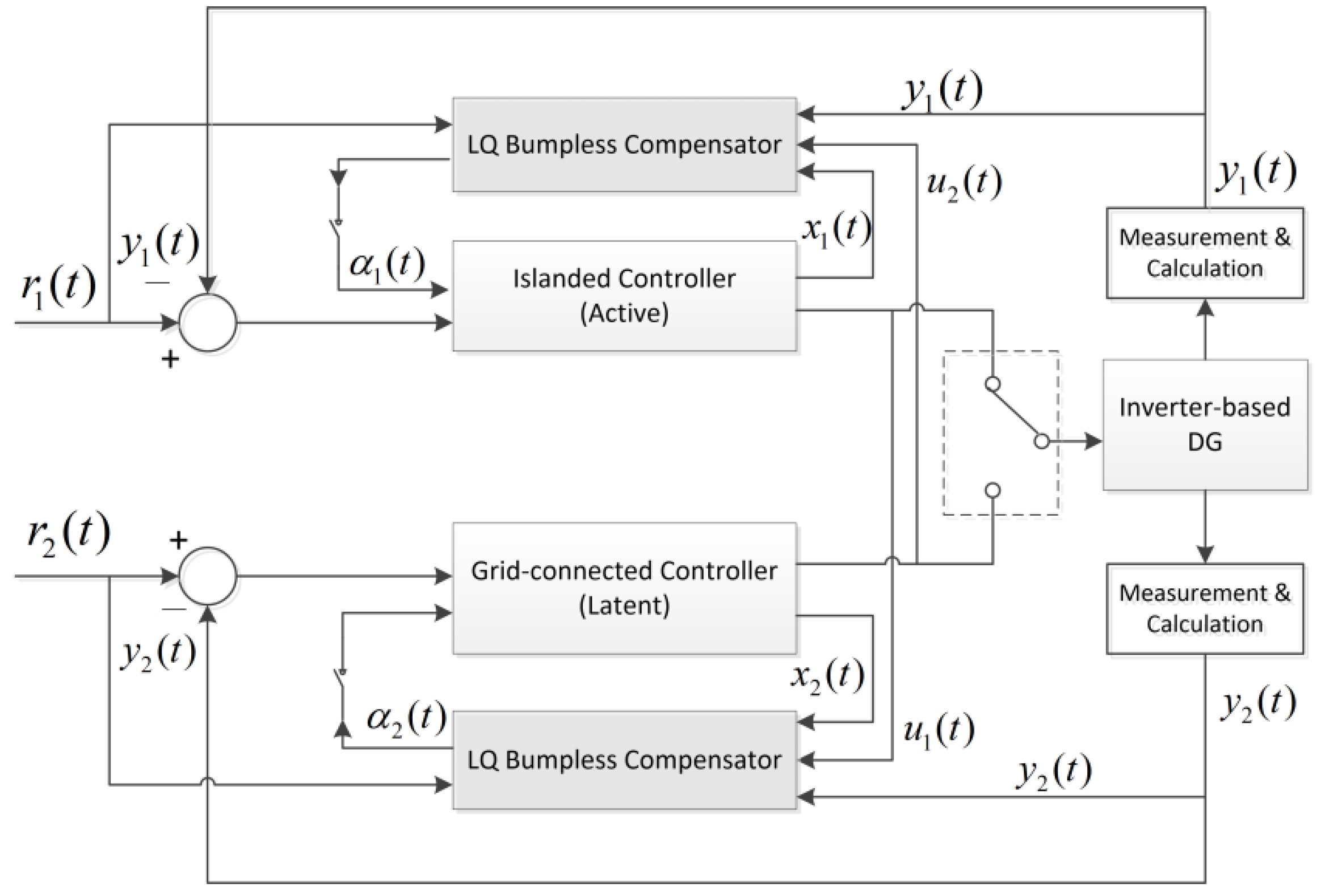
Figure 1 shows the scheme of a switched microgrids system with two candidate controllers under the bumpless transfer control strategy. It can be seen that there are two conditions needed to be satisfied to achieve a minimal transient jumping deviation when mode switching happens:

• The plant is driven by the output of active controller $u_a(t)$ and the plant input is switching from active controller to latent controller when the mode changes. Therefore, the two controllers should produce control output signals $u_a(t)$ and $u_l(t)$ as close as possible to each other, which will reduce the disturbance of the transient process. That can be expressed as $\underset{t\to \infty }{\lim }\left|u_l(t)-u_a(t)\right|=0$. This is the condition for output signals of two controllers.
• The active controller and the latent controller are driven by different signals. The active controller is triggered by reference tracking error with one DOF and the latent controller is triggered by reference mode error and bumpless compensator with two DOF. At the time of switching, when the controller is switching from the active to the latent, the driven signal for latent controller is switched from the bumpless compensator output $\alpha (t)$ and the reference mode error $e_a(t)$ to the reference tracking error $e_y(t)$. Therefore, to avoid large disturbance and maintain a good transient performance, we need to minimize these two kinds of driven signals, that is $\underset{t\to \infty }{\lim }\left|B_{l_1}{e}_a(t)+B_{l_2}\alpha (t)-B_a{e}_y(t)\right|=0$.

Thus, according to the above two control goals, a LQ optimal tracking control problem is formulated as follows.

The quadratic performance cost function for the design of bumpless transfer compensatory controller is written as:

$$J=\frac{1}{2}{\displaystyle {\int }_0^T[}{(u_l(t)-u_a(t))}^{T}Q(u_l(t)-u_a(t))+{(B_{l_1}{e}_a(t)+B_{l_2}\alpha (t)-B_a{e}_y(t))}^{T}R(B_{l_1}{e}_a(t)+B_{l_2}\alpha (t)-B_a{e}_y(t))]dt$$

(4)

where $u_a(t)$ and $u_l(t)$ are the outputs of active controller and latent controller, respectively. $Q$ and $R$ are corresponding positive weighting matrices.

The purpose of this paper is to find a bumpless transfer compensatory controller ${\alpha }^{*}(t)$ that can obtain the minimization of the performance cost index (4) subject to the equality constraints, as given by (1). We used the lagrangian multipliers method to solve the minimum problem with equality constraints. Combining (1), a lagrangian multiplier $\lambda (t)\in {ℝ}^n$ is introduced to construct an augmented functional $\widehat{J}$ as follows

$$\begin{array}{l}\widehat{J}=\frac{1}{2}{\displaystyle {\int }_0^T[}({(u_l(t)-u_a(t))}^{T}Q(u_l(t)-u_a(t))+{(B_{l_1}{e}_a(t)+B_{l_2}\alpha (t)-B_a{e}_y(t))}^{T}R(B_{l_1}{e}_a(t)+B_{l_2}\alpha (t)-B_a{e}_y(t)))\\ +{\lambda }^T(t)(A_l{x}_l(t)+B_{l_1}{e}_a(t)+B_{l_2}\alpha (t)-{\dot{x}}_l(t))]dt\end{array}$$

(5)

Forming the Hamiltonian $H(t)$ as follows

$$\begin{array}{ll}H(t)& =\frac{1}{2}({(u_l(t)-u_a(t))}^{T}Q(u_l(t)-u_a(t))+{(B_{l_1}{e}_a(t)+B_{l_2}\alpha (t)-B_a{e}_y(t))}^{T}R(B_{l_1}{e}_a(t)+B_{l_2}\alpha (t)-B_a{e}_y(t)))\\ & +{\lambda }^T(t)(A_l{x}_l(t)+B_{l_1}{e}_a(t)+B_{l_2}\alpha (t))\\ & =\frac{1}{2}({(C_l{x}_l(t)+D_{l_1}{e}_a(t)+D_{l_2}\alpha (t)-u_a(t))}^{T}Q(C_l{x}_l(t)+D_{l_1}{e}_a(t)+D_{l_2}\alpha (t)-u_a(t))\\ & +{(B_{l_1}{e}_a(t)+B_{l_2}\alpha (t)-B_a{e}_y(t))}^{T}R(B_{l_1}{e}_a(t)+B_{l_2}\alpha (t)-B_a{e}_y(t)))\\ & +{\lambda }^T(t)(A_l{x}_l(t)+B_{l_1}{e}_a(t)+B_{l_2}\alpha (t))\end{array}$$

(6)

Then augmented function $\widehat{J}$ can be rewritten as

$$\widehat{J}={\displaystyle {\int }_0^T[}H(t)-{\lambda }^T(t){\dot{x}}_l(t))]dt$$

(7)

For existence of a minimum of $\widehat{J}$, the necessary conditions should satisfy

$$\frac{\partial H}{\partial \lambda }={\dot{x}}_l$$

(8)

$$\frac{\partial H}{\partial x_l}=-\dot{\lambda }$$

(9)

$$\frac{\partial H}{\partial \alpha }=0$$

(10)

Equation (8) is state equation. Equation (9) is co-state equation. Combining Equation (3) with Equation (10), we have

$$\begin{array}{l}\frac{\partial H}{\partial \alpha }=0\Rightarrow D_{l_2}^{T}Q{D}_{l_2}\alpha +D_{l_2}^{T}Q{C}_l{x}_l+D_{l_2}^{T}Q{D}_{l_1}{e}_a-D_{l_2}^{T}Q{u}_a\\ +B_{l_2}^{T}R{B}_{l_2}\alpha +B_{l_2}^{T}R{B}_{l_1}{e}_a-B_{l_2}^{T}R{B}_a{e}_y+B_{l_2}^T\lambda =0\\ \therefore \alpha =M(D_{l_2}^{T}Q{u}_a+B_{l_2}^{T}R{B}_{l_1}{e}_y-D_{l_2}^{T}Q{C}_l{x}_l-(D_{l_2}^{T}Q{D}_{l_1}+B_{l_2}^{T}R{B}_{l_1})e_a-B_{l_2}^T\lambda )\end{array}$$

(11)

where

$$M={(D_{l_2}^{T}Q{D}_{l_2}+B_{l_2}^{T}R{B}_{l_2})}^{-1}$$

(12)

From co-state equation, combining (4), we have

$$\frac{\partial H}{\partial x_l}=-\dot{\lambda }\Rightarrow C_l^{T}Q{C}_l{x}_l+C_l^{T}Q{D}_{l_2}^{}\alpha +C_l^{T}Q{D}_{l_1}{e}_a-C_l^{T}Q{u}_a+A_l^T\lambda =-\dot{\lambda }$$

(13)

Suppose

$$\lambda =P{x}_l-g$$

(14)

where $P$ is known as the Riccati coefficient and $g\in {ℝ}^n$ is an adjoint vector to be solved. Substituting (11) and (14) into (13), we have

$$\begin{array}{ll}\dot{\lambda }& =-C_l^{T}Q{C}_l{x}_l-C_l^{T}Q{D}_{l_1}{e}_a-C_l^{T}Q{D}_{l_2}^{}M\left[D_{l_2}^{T}Q{u}_a+B_{l_2}^{T}R{B}_a{e}_y-D_{l_2}^{T}Q{C}_l{x}_l-(D_{l_2}^{T}Q{D}_{l_1}+B_{l_2}^{T}R{B}_{l_1})e_a-B_{l_2}^T(P{x}_l-g)\right]\\ & +C_l^{T}Qu-A_l^T(P{x}_l-g)\end{array}$$

(15)

And then, differentiating (14) on both sides, we can get

$$\dot{\lambda }=\dot{P}{x}_l+P{\dot{x}}_l-\dot{g}$$

(16)

Substituting (11) into (2), and then inserting them into (16), we have

$$\begin{array}{ll}\dot{\lambda }& =\dot{P}{x}_l+P[A_l{x}_l+B_{l_1}{e}_a+B_{l_2}M{D}_{l_2}^{T}Q{u}_a+B_{l_2}M{B}_{l_2}^{T}R{B}_a{e}_y-B_{l_2}M{D}_{l_2}^{T}Q{C}_l{x}_l\\ & -B_{l_2}M(D_{l_2}^{T}Q{D}_{l_1}+B_{l_2}^{T}R{B}_{l_1})e_a-B_{l_2}M{B}_{l_2}^{T}P{x}_l+B_{l_2}Mg]-\dot{g}\end{array}$$

(17)

Combining (15) and (17), the coefficients of $x_l$ in these two equations should be the same, and then we have

$$\begin{array}{l}\dot{P}+P{A}_l-P{B}_{l_2}M{D}_{l_2}^{T}Q{C}_l-P{B}_{l_2}M{B}_{l_2}^{T}P\\ =-C_l^{T}Q{C}_l+C_l^{T}Q{D}_{l_2}^{}M{D}_{l_2}^{T}Q{C}_l+C_l^{T}Q{D}_{l_2}^{}M{B}_{l_2}^{T}P-A_l^{T}P\end{array}$$

(18)

Based on (18), furthermore, we can obtain the famous differential Riccati equation as follows

$$\begin{array}{ll}-\dot{P}& =P{A}_l+A_l^{T}P-P{B}_{l_2}M{B}_{l_2}^{T}P-P{B}_{l_2}M{D}_{l_2}^{T}Q{C}_l-C_l^{T}Q{D}_{l_2}^{}M{B}_{l_2}^{T}P\\ & +C_l^{T}Q{C}_l-C_l^{T}Q{D}_{l_2}^{}M{D}_{l_2}^{T}Q{C}_l\end{array}$$

(19)

Equating the other coefficients of (15) and (16), we can have the following equation for $\dot{g}$

$$\begin{array}{ll}-\dot{g}& =(A_l^T-C_l^{T}Q{D}_{l_2}^{}M{B}_{l_2}^T-P{B}_{l_2}M)g\\ & +(P{B}_{l_2}M{D}_{l_2}^{T}Q{D}_{l_1}-P{B}_{l_2}M{B}_{l_2}^{T}R{B}_{l_1}-P{B}_{l_1}-C_l^{T}Q{D}_{l_1}^{}+C_l^{T}Q{D}_{l_2}^{}M{D}_{l_2}^{T}Q{D}_{l_1}+C_l^{T}Q{D}_{l_2}^{}M{B}_{l_2}^{T}R{B}_{l_1}^{})e_a\\ & +(C_l^{T}Q{D}_{l_2}^{}M{B}_{l_2}^{T}R{B}_a-P{B}_{l_2}M{B}_{l_2}^{T}R{B}_a)e_y+(C_l^{T}Q-P{B}_{l_2}M{D}_{l_2}^{T}Q-C_l^{T}Q{D}_{l_2}M{D}_{l_2}^{T}Q)u_a\end{array}$$

(20)

Then we can do the following definitions for the convenience of future calculation:

$$\begin{array}{l}N=(A_l^T-P{B}_{l_2}M-C_l^{T}Q{D}_{l_2}^{}M{B}_{l_2}^T{)}^{-1}\\ {\Omega }_a=P{B}_{l_2}M{D}_{l_2}^{T}Q{D}_{l_1}-P{B}_{l_2}M{B}_{l_2}^{T}R{B}_{l_1}-P{B}_{l_1}-C_l^{T}Q{D}_{l_1}^{}+C_l^{T}Q{D}_{l_2}^{}M{D}_{l_2}^{T}Q{D}_{l_1}+C_l^{T}Q{D}_{l_2}^{}M{B}_{l_2}^{T}R{B}_{l_1}^{}\\ {\Omega }_y=C_l^{T}Q{D}_{l_2}^{}M{B}_{l_2}^{T}R{B}_a-P{B}_{l_2}M{B}_{l_2}^{T}R{B}_a\\ \Phi =C_l^{T}Q-P{B}_{l_2}M{D}_{l_2}^{T}Q-C_l^{T}Q{D}_{l_2}M{D}_{l_2}^{T}Q\end{array}$$

(21)

When $T$ in Equation (7) tends to infinity, the Riccati coefficient has a solution on the steady state. Thus, when $T\to \infty$, $\dot{P}\to 0$, $\dot{g}\to 0$, then from (19) and (20), we have

$$\begin{array}{ll}0& =P{A}_l+A_l^{T}P-P{B}_{l_2}M{B}_{l_2}^{T}P-P{B}_{l_2}M{D}_{l_2}^{T}Q{C}_l-C_l^{T}Q{D}_{l_2}^{}M{B}_{l_2}^{T}P\\ & +C_l^{T}Q{C}_l-C_l^{T}Q{D}_{l_2}^{}M{D}_{l_2}^{T}Q{C}_l\end{array}$$

(22)

$$\begin{array}{l}0=N^{-1}g+{\Omega }_a{e}_a+{\Omega }_y{e}_y+\Phi u_a\\ \Rightarrow g=-N({\Omega }_a{e}_a+{\Omega }_y{e}_y+\Phi u_a)\end{array}$$

(23)

where $P$ can be obtained by the solution of algebraic Riccati Equation (22).

Once $P$ and $g$ are obtained from (22) and (23), the Lagrange coefficient $\lambda$ can be calculated from (14) by substituting $P$ and $g$ into (14). Then the bumpless transfer compensator output $\alpha (t)$ can be determined by (11) and furthermore can be expressed as follows for infinite time horizon.

$$\alpha =G{\left[\begin{array}{cccc}{x}_l& u_a& e_a& e_y\end{array}\right]}^T$$

(24)

where the Matrix $G$ is given by

$$G=M{\left[\begin{array}{c}{(-D_{l_2}^{T}Q{C}_l-B_{l_2}^{T}P)}^T\\ {(D_{l_2}^{T}Q-N\Phi )}^T\\ {(-D_{l_2}^{T}Q{D}_{l_1}-B_{l_2}^{T}R{B}_{l_1}-N{\Omega }_a)}^T\\ {(B_{l_2}^{T}N{B}_a+N{\Omega }_y)}^T\end{array}\right]}^T$$

(25)

From (25) we can see that the matrix of the bumpless transfer compensator is time invariant, which can be calculated out off-line. This bumpless transfer compensator will trigger the latent controller tracking the active controller in real time, and as soon as switching happens, the active controller can be smoothly transferred to the latent controller.

3. Application of Optimal Bumpless Transfer Control in Microgrids

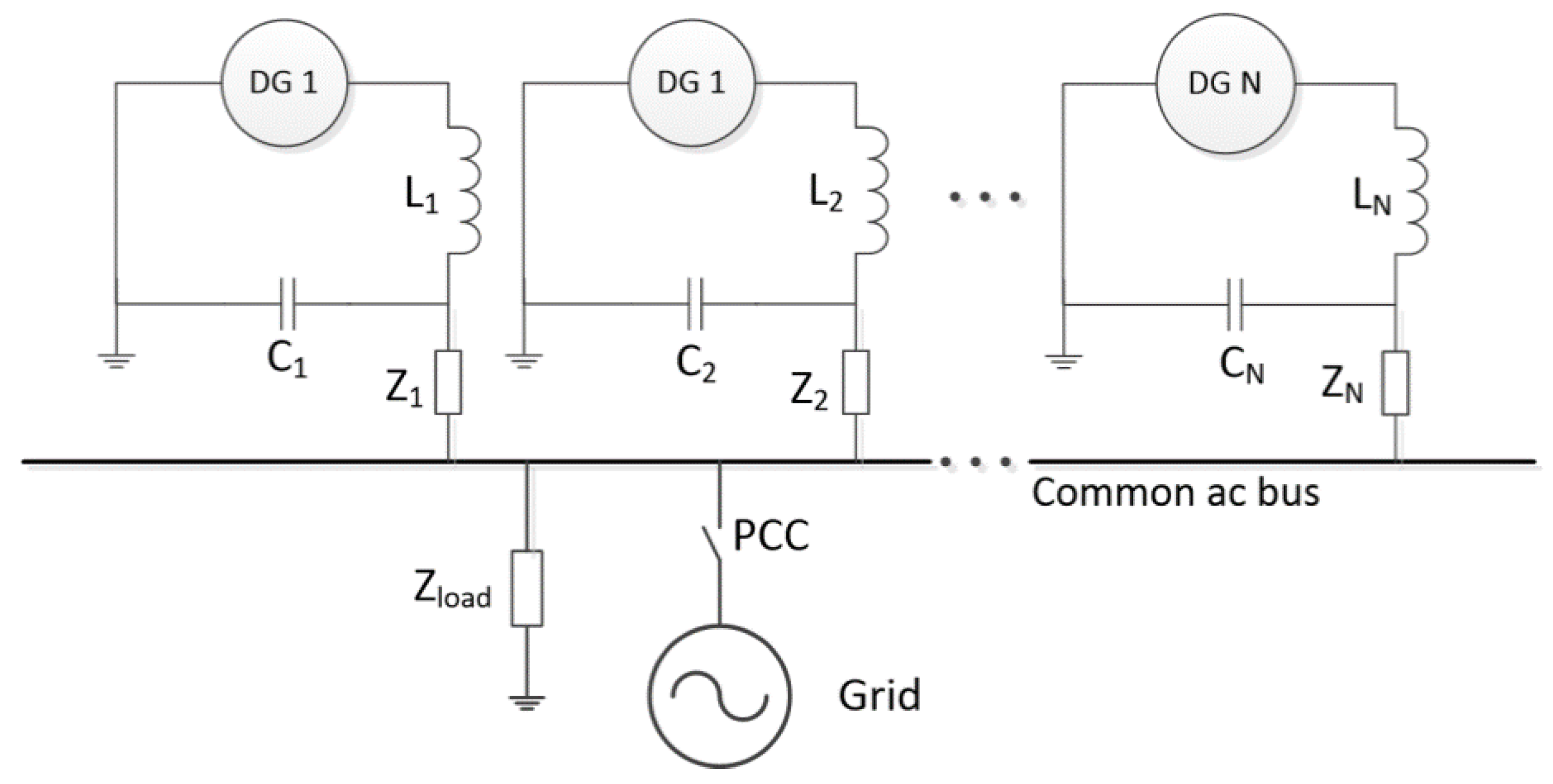
In this section, the proposed LQ-based bumpless transfer controller with two DOF is applied to the AC microgrids with two operation modes. The structure of the AC microgrids contains three parts: the inverter-based DG model, the line feeder model, and the microgrids network model. The equivalent power circuit is shown in Figure 2.

As mentioned above, two bumpless transfer compensatory controllers need to be designed respectively for the two operation modes. In the following section, we will discuss how to design this mode dependent LQ optimal bumpless compensator.

3.1. Islanded Operation Mode

In the islanded microgrids, the effect of the feeder impedance mismatch needs to be considered and compensated by extra control strategies. To overcome the drawback of the traditional droop control method, the current-based PI controller is designed in this paper to adjust the deviation caused by the traditional droop. Thus, the droop algorithm for inverter n can be modified into the following form.

$$\begin{array}{l}{\omega }_n={\omega }_n^{*}-m_n(I_{dn}-I_{dn}^{*}+\delta I_{dn})\\ E_n=E_n^{*}-n_n(I_{qn}-I_{qn}^{*}+\delta I_{qn})\end{array}$$

(26)

where ${\omega }_n^{*}$, $E_n^{*}$, $I_{dn}^{*}$, and $I_{qn}^{*}$ are the reference values. $m_n$ and $n_n$ are the droop parameters. $I_{dn}^{}$ and $I_{qn}^{}$ are the measured current. $\delta I_{dn}$ and $\delta I_{qn}$ are the compensate control inputs generated from the current-based PI controller, which can be expressed as

$$\begin{array}{l}\delta I_{dn}=k_{Pdn}(I_{dn}(t)-I_{dn}^{*}(t))+k_{Idn}{\displaystyle {\int }_0^t(I_{dn}(\tau )-I_{dn}^{*}(\tau ))}d\tau \\ \delta I_{qn}=k_{Pqn}(I_{qn}(t)-I_{qn}^{*}(t))+k_{Iqn}{\displaystyle {\int }_0^t(I_{qn}(\tau )-I_{qn}^{*}(\tau ))}d\tau \\ I_{dn}^{*}=\frac{{\displaystyle \sum _{n=1}^N{I}_{dn}}}{N},I_{qn}^{*}=\frac{{\displaystyle \sum _{n=1}^N{I}_{qn}}}{N}\end{array}$$

(27)

In this method, each inverter measures the output current and sends it to others to calculate the average current $I_{dn}^{*}$ and $I_{qn}^{*}$ to generate the compensate control value $\delta I_{dn}$ and $\delta I_{qn}$ from the PI controller, which will be finally sent to the current-based droop controller.

Based on the designed islanded PI controller above, to obtain the bumpless transfer compensatory controller $\alpha (t)$ of (2), we need to derive a state–space model of the current-based PI controller (27) and transform it into the standard state–space from as (1).

Define auxiliary state variables for both active and reactive current of inverter n as follows.

$$\{\begin{array}{l}{x}_{adn}={\displaystyle {\int }_0^t(I_{dn}(\tau )-I_{dn}^{*}(\tau ))}d\tau \\ x_{aqn}={\displaystyle {\int }_0^t(I_{qn}(\tau )-I_{qn}^{*}(\tau ))}d\tau \end{array}$$

(28)

Then, from (1) and (27), we can derive the coefficients of the state–space function (1) for both active and reactive currents as follows.

$$\begin{array}{l}\{\begin{array}{l}{A}_{adn}=0,B_{adn}=I,C_{adn}=k_{Idn},D_{adn}=k_{Pdn}\\ A_{aqn}=0,B_{aqn}=I,C_{aqn}=k_{Iqn},D_{aqn}=k_{Pqn}\end{array}\\ and\\ \{\begin{array}{l}{r}_{an}=I_{dn}^{*},y_{dn}=I_{dn}\\ r_{an}=I_{qn}^{*},y_{qn}=I_{qn}\end{array}\end{array}$$

(29)

where $k_{Idn},k_{Pdn}$ and $k_{Iqn},k_{Pqn}$ are the parameters of PI controller.

Finally, the proposed dynamic adaptive bumpless transfer compensatory algorithm in Section 2 is applied to (29) to get the bumpless transfer compensator output $\alpha (t)$, which will trigger the latent islanded controller, fast-tracking the active grid connected controller to achieve the smooth transfer when the switching happens.

3.2. Grid Connected Operation Mode

In this case, the parallel connected inverters not only need to keep system frequency and system voltage following the main grid, but only needs to supply constant P and Q as required. To track the given reference $P^{*}$ and $Q^{*}$, firstly we need to calculate the instantaneous output power of inverter as follows.

$$\begin{array}{l}p=\frac{3}{2}(E_{dn}{I}_{dn}+E_{qn}{I}_{qn})\\ q=\frac{3}{2}(E_{dn}{I}_{qn}-E_{qn}{I}_{dn})\end{array}$$

(30)

where $E_{dn}$ and $E_{qn}$ are the inverter n’s output voltage of d and q axis. $I_{dn}$ and $I_{qn}$ are the inverter n’s output current of d and q axis.

Secondly, the average power from LPF is calculated by

$$P=\frac{{\omega }_c}{s+{\omega }_c}p,Q=\frac{{\omega }_c}{s+{\omega }_c}q$$

(31)

Thirdly, to control the power output P and Q to track the given reference $P^{*}$ and $Q^{*}$, we incorporated $P-\omega$ and $Q-E$ droop characteristics to design a power-based PI controller and achieve the operation objectives of grid connected mode by regulating frequency and output voltage for each inverter. The control algorithm can be expressed as follows.

$$\begin{array}{l}\delta {\omega }_n=k_{PPn}(P_n(t)-P_n^{*}(t))+k_{IPn}{\displaystyle {\int }_0^t(P_n(\tau )-P_n^{*}(\tau ))}d\tau \\ \delta E_n=k_{PQn}(Q_n(t)-Q_n^{*}(t))+k_{IQn}{\displaystyle {\int }_0^t(Q_n(\tau )-Q_n^{*}(\tau ))}d\tau \\ and\\ {\omega }_n={\omega }_n^{*}-m_n(P_n-P_n^{*})+\delta {\omega }_n\\ E_{dn}=E_{dn}^{*}-n_n(Q_n-Q_n^{*})+\delta E_n\\ E_{qn}^{*}=0\end{array}$$

(32)

Based on the designed grid connected PI controller above, to obtain the bumpless transfer compensatory controller $\alpha (t)$ according to the latent controller form (2), firstly we need to derive a state–space model of the power-based PI controller (32) and equivalently transform into the standard state–space from (1).

We define auxiliary power-related state variables of inverter n as follows.

$$\{\begin{array}{l}{x}_{lPn}={\displaystyle {\int }_0^t(P_n(t)-P_n^{*}(t))}d\tau \\ x_{lQn}={\displaystyle {\int }_0^t(Q_n(t)-Q_n^{*}(t))}d\tau \end{array}$$

(33)

Then from (2) and (33), we can derive the coefficients of the state–space function (2) for both active and reactive current as follows.

$$\begin{array}{l}\{\begin{array}{l}{A}_{aPn}=0,B_{aPn}=I,C_{aPn}=k_{IPn},D_{aPn}=k_{PPn}\\ A_{aQn}=0,B_{aQn}=I,C_{aQn}=k_{IQn},D_{aQn}=k_{PQn}\end{array}\\ and\\ \{\begin{array}{l}{r}_{aPn}=P_n^{*},y_{Pn}=P_n\\ r_{aQn}=Q_n^{*},y_{Qn}=Q_n\end{array}\end{array}$$

(34)

where $k_{IPn},k_{PPn}$ and $k_{IQn},k_{PQn}$ are the parameters of PI controller.

Finally, the proposed dynamic adaptive bumpless transfer compensatory algorithm in Section 2 is applied to (34) to obtain the bumpless transfer compensator output $\alpha (t)$, which will trigger the latent grid connected controller, fast-tracking the active islanded controller to achieve the smooth transfer when the switching happens.

4. Simulations

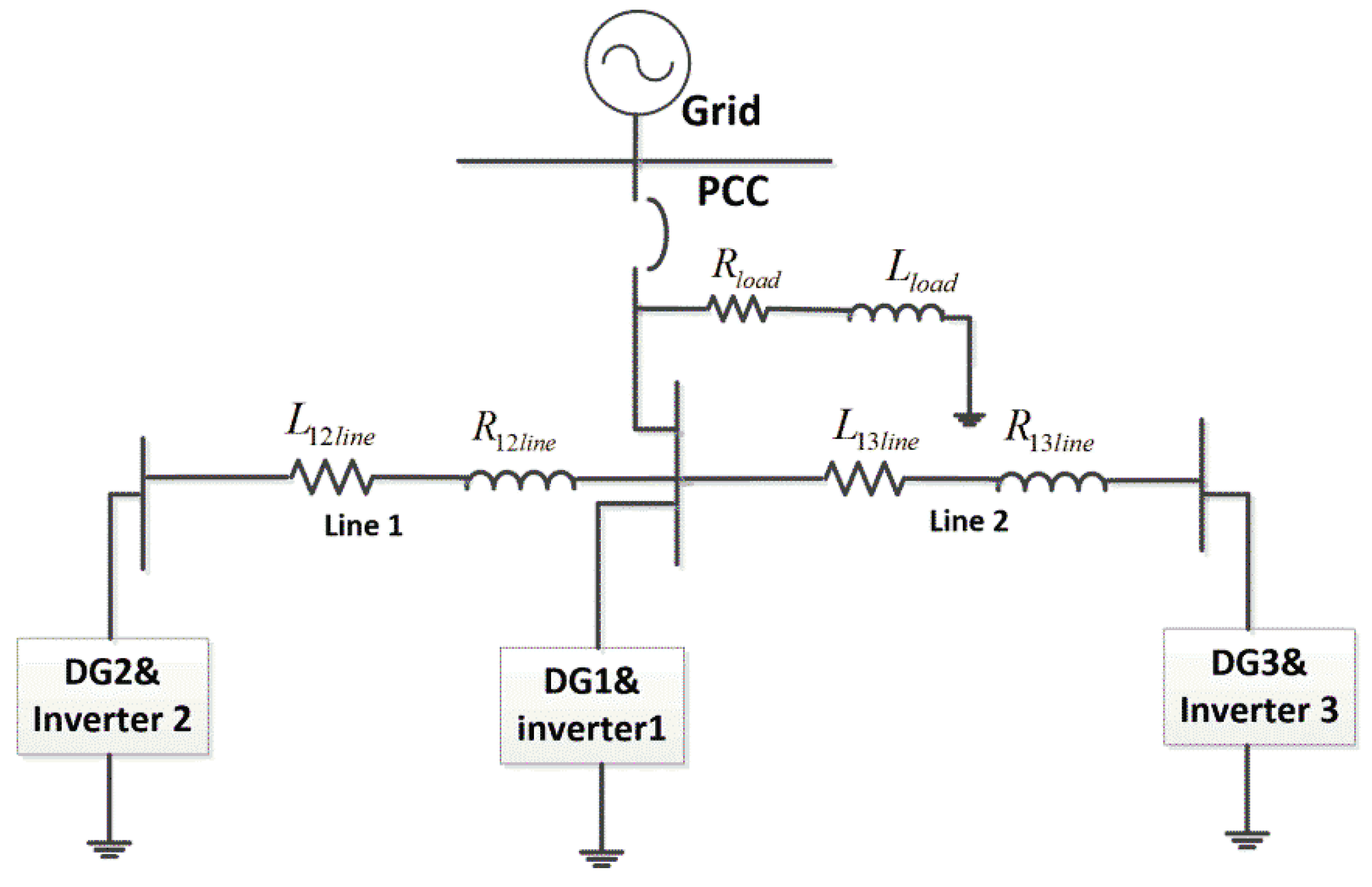
In this section, to validate the proposed mode-dependent bumpless transfer control strategy, a prototype microgrids (220 V, 50 Hz) with three inverters was built in SIMULINK. Figure 3 shows the structure. These inverters are controlled by distributed mode-dependent controllers.

To achieve bumpless transfer, two bumpless compensators need to be designed separately based on the proposed strategy in this paper. The specific calculation steps are as follows.

Step 1: obtain the state space model of the latent island controller. In this case, the current operation mode is grid connected mode. The system matrix of this state space model can be obtained from (29), where the parameters of PI controller $k_{Idn},k_{Pdn}$ and $k_{Iqn},k_{Pqn}$ can be tuned by Matlab PID control tuner app.

Step 2: obtain the state space model of the latent grid connected controller. In this case, the current operation mode is islanded mode. The system matrix of this state space model can be obtained from (34). Where the parameters of PI controller $k_{IPn},k_{PPn}$ and $k_{IQn},k_{PQn}$ can be tuned by Matlab PID control tuner app.

Step 3: obtain $P$ by the solution of algebraic Riccati equation (22) by using care command in Matlab.

Step 4: once $P$ is obtained, $g$ can be calculated from (23).

Step 5: calculate the Lagrange coefficient $\lambda$ from (14) by substituting $P$ and $g$ into (14).

Step 6: compute the feedback matrix $G$ from (25).

Step 7: determine the bumpless transfer compensator output $\alpha (t)$ by (25).

Three test cases were carried out.

Table 1. Microgrids system parameters.

Parameter	Value	Parameter	Value	Parameter	Value
Common bus voltage	220 V	System frequency	50 Hz	Droop control m1 = m2 = m3	$2.5\times {10}^{-3}$
DC–Input voltage	300 V	AC–Output voltage	220 V	Droop control n1 = n2 = n3	$3.5\times {10}^{-5}$
Capacity of inverter 1	3 KW	Capacity of inverter 2	3 KW	Capacity of inverter 3	3 KW
Filter 1 inductance	0.6 mH	Filter 2 inductance	0.6 mH	Filter 3 inductance	0.6 mH
Filter 1 capacitor	10 μF	Filter 2 capacitor	10 μF	Filter 3 capacitor	10 μF
Line 1 resistor	0.2 ohm	Line 2 resistor	0.2 ohm	Load resistor	150 ohm
Line 1 inductor	0.6 mH	Line 2 inductor	0.6 mH	Load inductor	0.3 mH

displays the system parameters of the microgrids network shown in Figure 3.

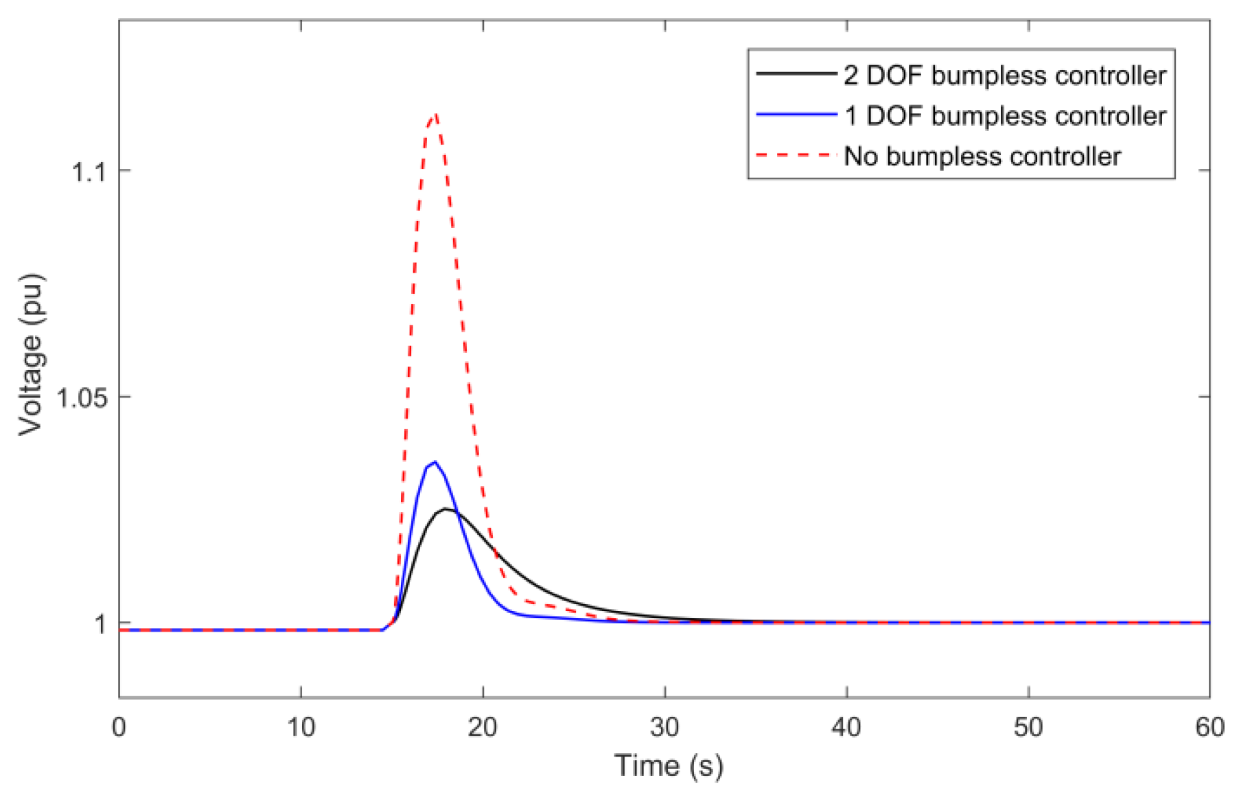
4.1. Case 1: Transition from Islanded Mode to Grid Connected Mode

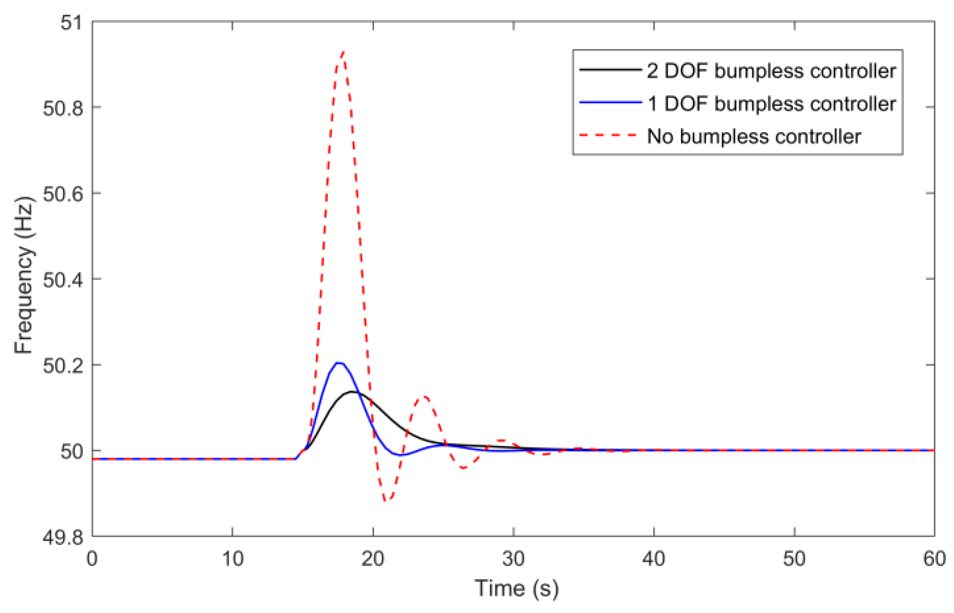
Initially, the microgrids operate in the islanded mode, then at t = 15 s, it connects to the main grid. The microgrids needs to be synchronized to the main grid. The results are shown in Figure 4 and Figure 5. Here, we make a comparison between the proposed two DOF bumpless control strategy and the one DOF bumpless control strategy used in [23].

From Figure 4 and Figure 5, we can see that the system frequency and the common bus voltage are fast-tracking the main grid to the nominal values after issuing the grid connection command. The maximum overshoot of frequency changes from 1.9% to 0.26% and the maximum overshoot of voltage changes from 11.7% to 2.3%. It is easy to see that the proposed two DOF bumpless transfer control strategy can fast drag the system back to the equilibrium point. Compared with the results of no compensator, it can be observed that the voltage peak is over 1.1 pu and the frequency peak is almost 51 Hz for a prolonged duration without any bumpless compensation. Furthermore, compared with the one DOF controller in [23], it has a better transient performance. The integral of squared error of frequency for these three cases are 3.5985, 0.2111, and 0.1443, respectively, and the integral of squared error of voltage for these three cases are 0.0646, 0.0064, and 0.0054, respectively. When operating in the grid connected mode, the frequency is settled to exactly 50 Hz and the PCC voltage is settled to 1 pu, which is the same as the voltage of the main grid.

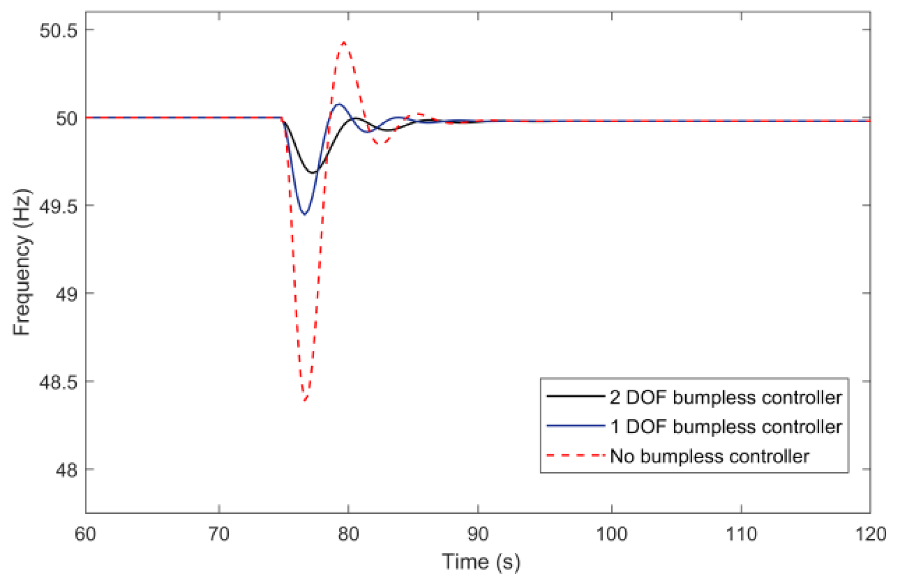
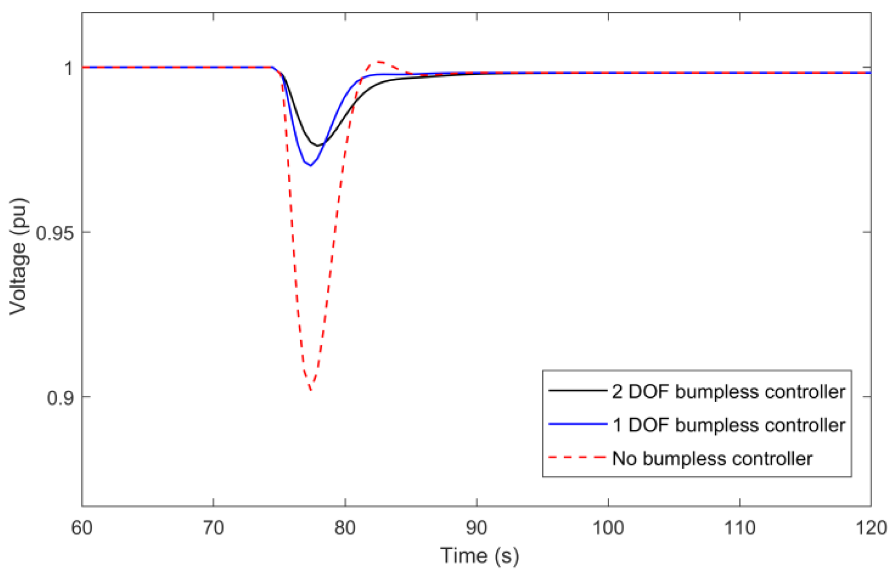
4.2. Case 2: Transition from Grid Connected Mode to Islanded Mode

At t = 75 s, microgrids disconnected from the main grid and operated in the islanded mode. The microgrids need to maintain the balance of system frequency and voltage. The results are shown in Figure 6 and Figure 7.

From Figure 6 and Figure 7, we can see that the microgrids system frequency and voltage dropped a little bit from the nominal value without the support of the main grid frequency and voltage after issuing the grid disconnection command. The maximum overshoot of frequency changed from 3.3% to 0.51% and the maximum overshoot of voltage changed from 9.5% to 2.2%. Compared with the results of no compensator, it can be observed that the voltage peak is over 0.9 pu and the frequency peak is over 47 Hz for a prolonged duration without any bumpless comparison. Furthermore, compared with the one DOF controller in [23], it has a better transient performance. It is easy to see that the proposed bumpless transfer control strategy can effectively restrict the transient behavior within a desirable limit. The integral of squared error of frequency for these three cases are 14.1613, 1.5336, and 0.6146, respectively, and the integral of squared error of voltage for these three cases are 0.0467, 0.0040, and 0.0032, respectively.

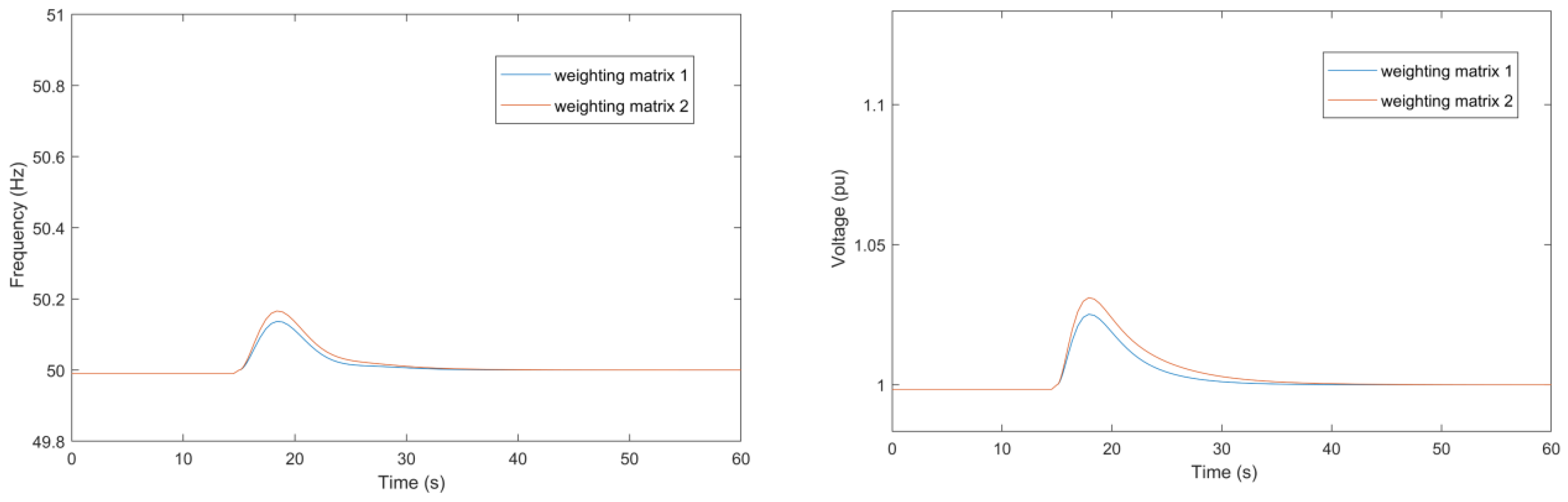
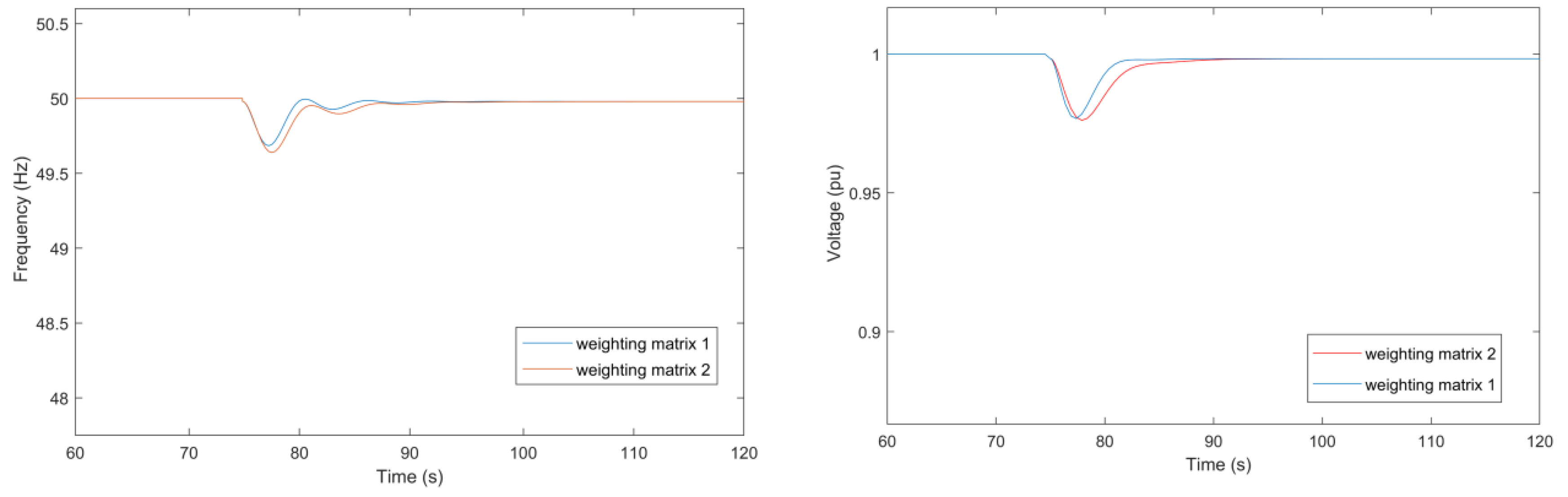
Weighting matrices Q and R in the quadratic performance cost function play a very important role in deciding the system transient performance. Here, we will do a small sensitivity study with the variation of R and Q. There are various methods reported in published literatures on how to select these weighing matrixes. We used the Bryson’s suggestion to select matrix R and Q [25] and do a comparison of two groups of Q and R. Comparison results are shown in Figure 8 and Figure 9.

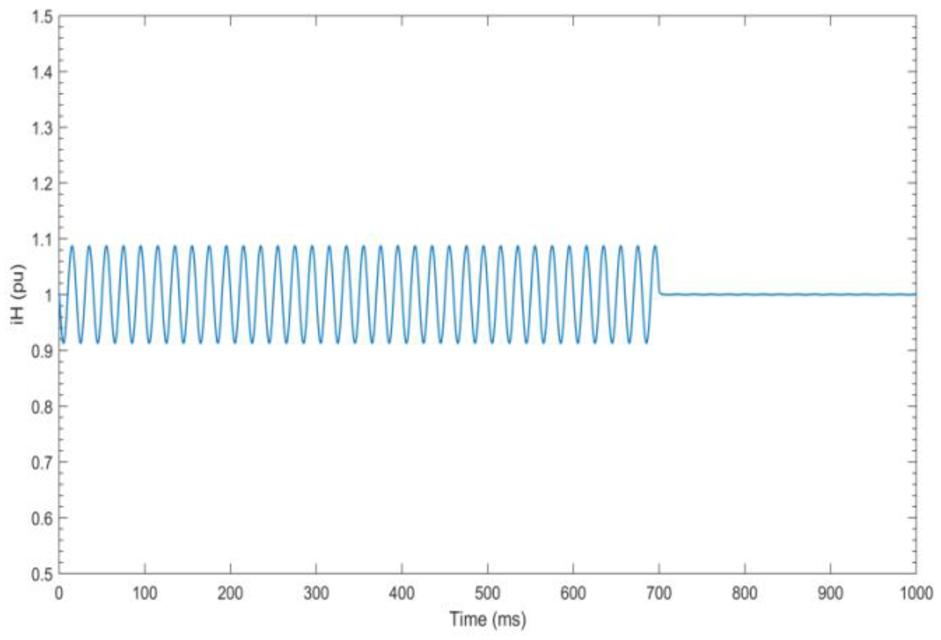
4.3. Case 3: Circulating Current When Line Impendences are Different

In order to validate the effectiveness of islanded mode controller after the system ran out of the main grid, we designed the case 3. In this case, the system initially operates in grid connected mode and at t = 700 ms it disconnected. After the bumpless compensator does its work, the islanded controller does its contribution to suppress the circulating current, even with the mismatches of the output impedance of each inverter. In this case, the resistors of Line 1 and Line 2 are different. Line 1 is 0.2 ohm and Line 2 is 0.4 ohm. The results of the circulating current of inverter 2 and inverter 3 are shown in Figure 10.

4.4. Case 4: More Complicated Transition Scenarios Validation

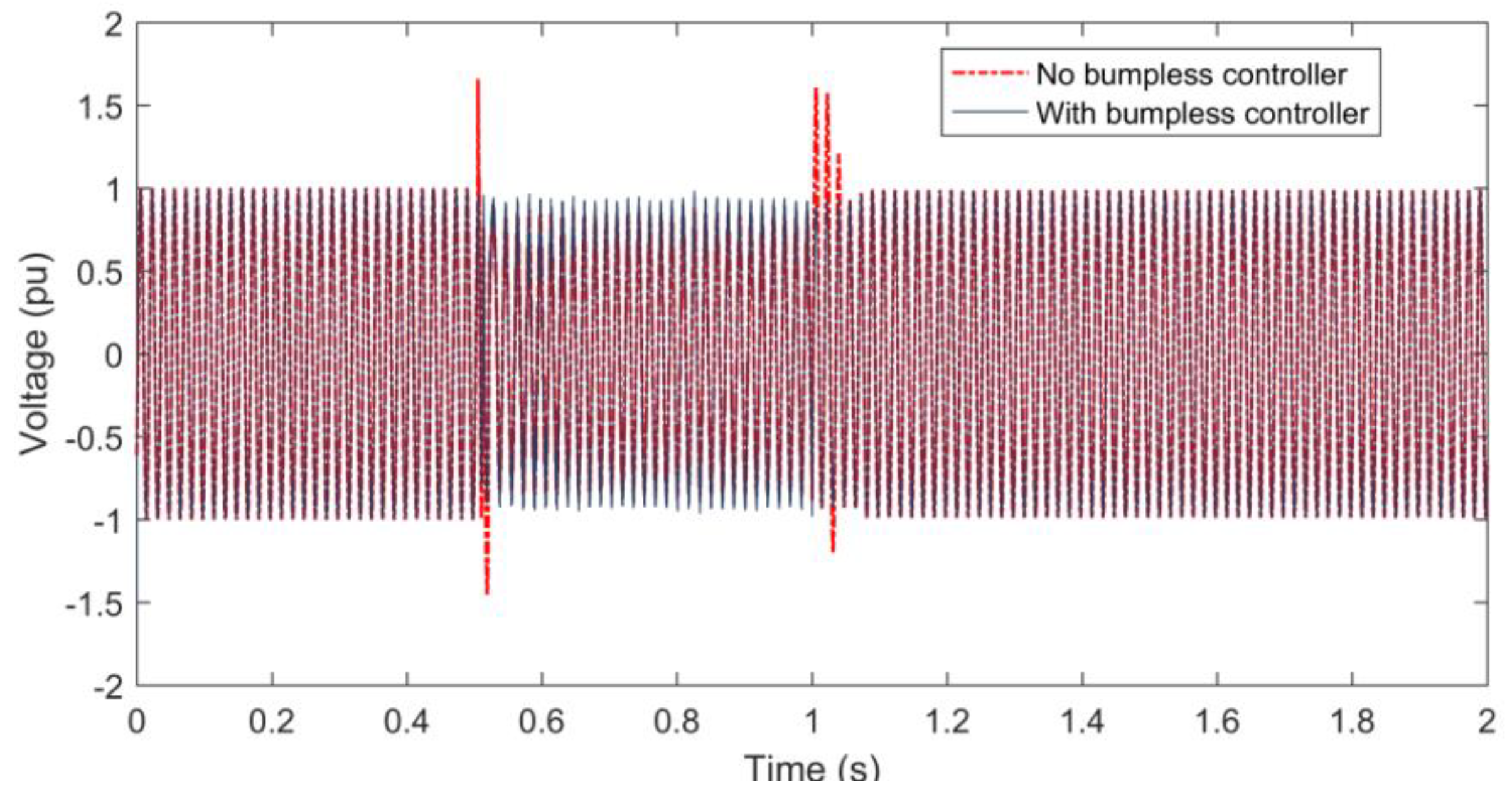
In this case, we enlarged the test case to a common medium voltage microgrids with more complicated transition scenarios. In this system, two 125 kw PV arrays were parallel connected via inverters to a 25 kv 60 Hz grid. To clearly show the transition performance of voltage amplitude, we will shorten the simulation time. The scenarios are as follows:

From t = 0 s to t = 0.5 s, microgrids operated in a grid connected mode. MPPT was used to keep the power almost constant at rated 125 kW by MPPT. At the beginning, load 1 is connected with P = 250 kW.

• At t = 0.5 s, microgrids ran out of the main grid and, meanwhile, the sun irradiance was ramped down from $1\mathrm{kw}/{\mathrm{m}}^2$ to $0.2\mathrm{kw}/{\mathrm{m}}^2$.
• At t = 1 s, microgrids were reconnected to the main grid.
• At t = 1.5 s, load 2 is on with P = 250 kW.
• At t = 2 s, the simulation stops.

From the scenarios, we can see that, initially, microgrids operate in the grid connected mode and the controller can synchronize the frequency and voltage safely with the main grid, as well as supply constant power as requested (250 kW required by load 1). Then at t = 0.5 s, microgrids is disconnected, this scenario is to check the effectiveness of islanded bumpless controller. Then at t = 1 s, microgrids is reconnected to the main grid, this scenario is to check the effectiveness of grid connected bumpless controller. Finally at t = 1.5 s, to check the impact of load change on power quality and the tracking performance of mode controller, load 2 (250 kW) is connected to the system.

Figure 11 shows the results of PCC voltage (phase A) response in the whole running process. Transition happens at t = 0.5 s from the grid connection to the islanded mode and at t = 1 s is connected back. We can see that the proposed bumpless controller successfully suppresses the transient jump and helps PCC voltage have a fast recovery to the stable stage with a slight drop from the nominal value without the support of the main grid.

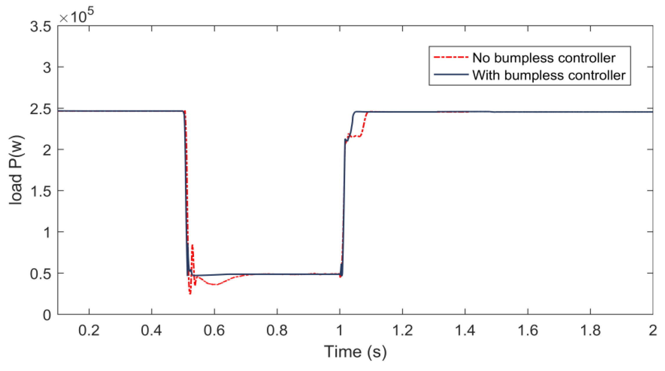
Figure 12 is the dynamics of active power of load 1. We can see that initially in grid connected mode, the load can work in their nominal point and the total consuming power is 250 kW, then at t = 0.5 s, microgrids is disconnected and meantime sun irradiance is ramped down from $1\mathrm{kw}/{\mathrm{m}}^2$ to $0.2\mathrm{kw}/{\mathrm{m}}^2$, we can see that only the PV system can provide power to load 1, so the total consuming power is reduced to about 50 kW. Then at t = 1 s, microgrids is reconnected to the main grid and it can support complementary power to load 1, so load 1 can work its nominal power again. During the transitions at t = 0.5 s and t = 1 s, we can see that the proposed bumpless controller effectively suppress the overshoots in transitions.

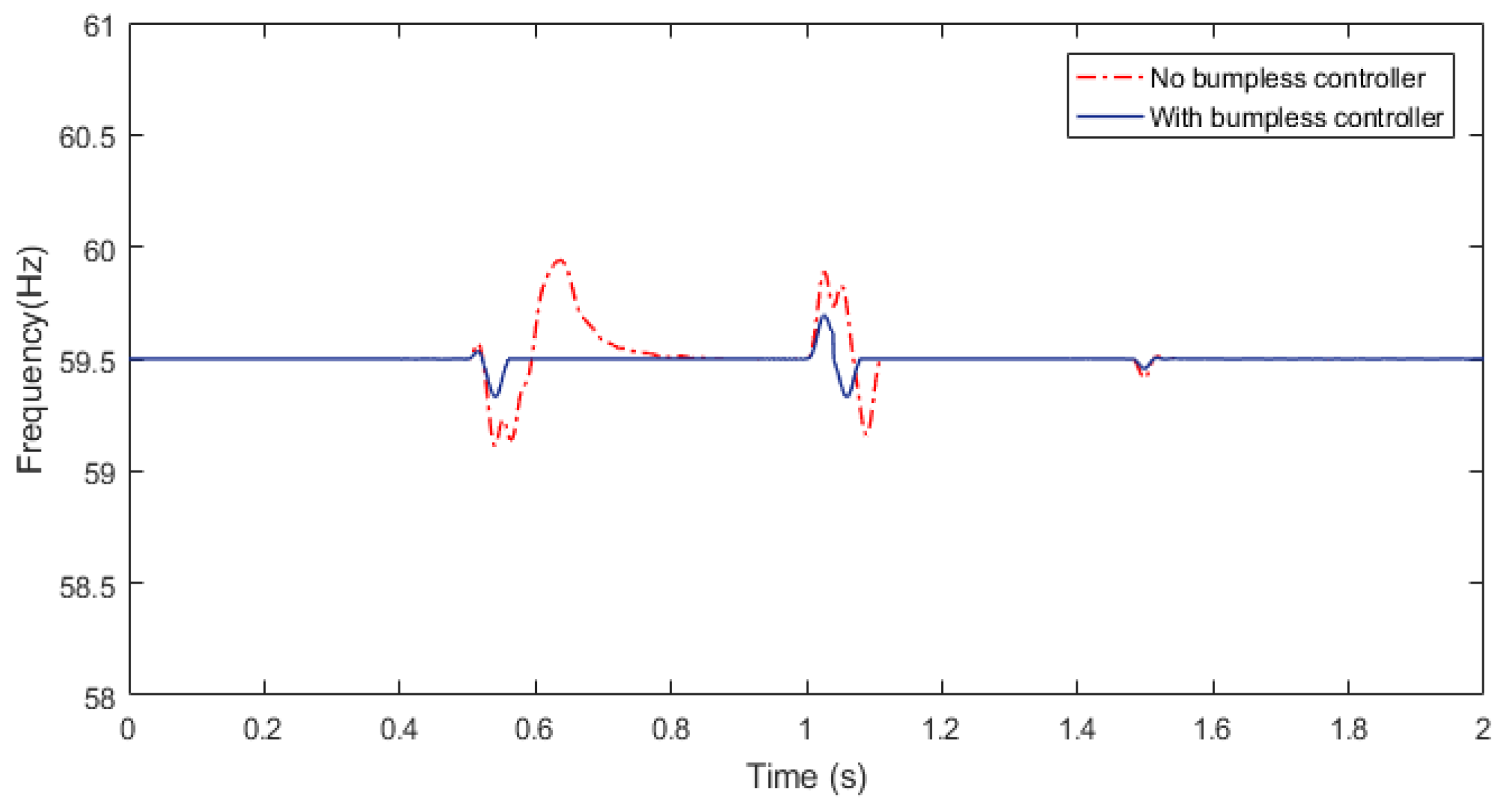
Figure 13 is the dynamics of the system frequency. During the switching, although there are some fluctuations produced, it is easy to see that the proposed bumpless transfer control strategy can help the system get a better transient behavior. We can see that the new added load (250 kW) also has a little impact on the system frequency and the proposed bumpless strategy can also reduce the overshoot in this load change transition, but it is not very effective. So in future work, we need to consider more transition cases to improve the performance of the bumpless control strategy.

5. Conclusions

In this paper, two separate controllers were designed for two operation modes of the microgrids. To deal with the problem of bumpless transfer for microgrids with these two operation modes, a two DOF bumpless controller was proposed to adaptively compensate the control input discontinuity and reference step when mode transfer happens. This bumpless algorithm is effectively forcing the latent controller tracking the active controller, as well as guaranteeing the plant output, tracking the reference as close as possible to achieve the continuity of the switching behavior by minimizing the transient performance criteria in terms of these two degrees of driven signals. Effectiveness of the proposed two DOF LQ-based bumpless transfer control strategy is validated from simulation results by comparisons with both the results of no bumpless controller and one DOF bumpless controller.