Article

Model-Independent Derivative Control Delay Compensation Methods for Power Systems

Room 157, School of Electrical and Electronic Engineering, University College Dublin, Belfield, Dublin 4, Ireland
*
Author to whom correspondence should be addressed.
Energies 2020, 13(2), 342; https://doi.org/10.3390/en13020342
Submission received: 5 December 2019 / Revised: 26 December 2019 / Accepted: 7 January 2020 / Published: 10 January 2020

Abstract

:
The paper examines the effectiveness of utilizing the derivatives of time delayed, wide-area signals in mitigating their destabilizing impact on power system dynamic response. In particular, the paper discusses two derivative control-based delay compensation methods, namely proportional-derivative (PD) and predictor-based delay compensation. The two methods are compared in terms of their open-loop signal fidelity and their impact on the closed-loop system stability. The paper also provides a technique to carry out small-signal stability analysis with inclusion of derivative control based compensation, which leads to a Neutral Time-Delay System (NTDS). In addition, we provide a new theorem on the stability of the NTDS. Finally, nonlinear time domain simulations and eigenvalue analysis based on the IEEE 14-bus and New England 39-bus systems were carried out for the sake of comparison of the two delay compensation methods.

1. Introduction

1.1. Motivation

Communication delays introduced into power systems can be divided into closed-loop and open-loop delays. Closed-loop delays appear in controllers fed by remote signals, such as in wide-area damping controllers [1,2]. These delays can significantly decrease the damping of oscillatory modes, and even lead to system collapse. Open-loop delays appear in on-line monitoring and stability assessment [3,4,5,6]. These delays distort the original signals and therefore result in errors for the on-line monitoring and stability assessment. These errors may mislead the Transmission System Operators (TSOs) and thus impact on the operation and reliability of the overall power system. Accordingly, the main objectives of delay compensation methods aiming at mitigating the negative impact of communication delays on power systems are twofold, namely to avoid the unstable issues resulting by the closed-loop delays and to improve the fidelity of the signals impacted by the open-loop delays. The derivative (D) term of the conventional PID controller has been proved to be a simple but effective method to compensate time-delays. Several D-term-based delay compensation methods have been developed [7,8,9]. Their application to power systems is limited, and no systematic method for their evaluation has been presented thus far. This paper proposes an approach to evaluate the effect of D-term-based delay compensation, on both closed-loop and open-loop delays in power systems.

1.2. Literature Review

1.2.1. Communication Delays in Power Systems

Communication delays in power systems result from a series of processes along the data communication, from the measurement device to the control center, including long-distance data delivery, data packet dropout, noise, communication network congestion, etc. [10]. Due to these phenomena, such delays are time-variant. For the sake of simplicity, many studies have considered communication delays as constant [11,12,13]. In [8,14,15], communication delays are modeled through stochastic processes. However, a precise delay model is required in order to obtain an accurate stability assessment of a time-delay system [16,17]. The authors of [10,18], with thorough discussions on the communication process of Wide-Area Measurement System (WAMS) and data from a real-world power system, pointed out that the magnitude of communication delays in power systems is affected by the random data packet dropout and stochastic network-induced latency. A data-packet based delay model that accounts for these random and stochastic issues is provided in [19]. In the remainder of the paper, D-term-based delay 43 compensation methods are tested with the realistic communication delay model proposed in [19].

1.2.2. Compensation of Delays in Control Loops

Robust wide-area controllers have been proposed to mitigate the negative impact of closed loop delays [20]. However, control design for improved robustness against time-delays may deteriorate the overall dynamic response of the system [21]. Consequently, conventional controllers with external delay compensation often perform better than robust controllers. Another approach that has been commonly utilized to compensate delays in control loops is the use of predictive controllers [22,23,24]. Nevertheless, most predictive controllers are model-dependent and, thus, their effectiveness relies on the availability of an accurate dynamic model and the parameters of the system, which is not the case in power systems. Therefore, model-independent delay compensation methods are more practical for 53 power system applications. Moreover, Chaudhuri et al., showed that the model-independent delay compensation methods can perform equally well or even better than model-dependent ones [25].

1.2.3. Compensation of Delays in on-Line Monitoring

The extent of similarity between an originally sent signal and the signal actually received can be expressed in terms of fidelity [26]. In common practice, fidelity is utilized as a measure of the degree of amplitude and phase angle deviations of the input signal of amplifiers. With this regard, delays impact on the amplitude and phase angle of a signal by introducing a time shift. Moreover, as we show in the example and case study, the delay compensation introduces an amplitude distortion which can be conveniently quantified in terms of fidelity. Finally, we note that, in the literature, fidelity has been already used in the context of delayed dynamic systems (see, e.g., [9]). Methods that focus on the improvement of signals fidelity have been rarely considered in the power system literature. Meanwhile, the communication system community focuses on achieving high signal fidelity through new technologies, such as 5G and quantum communication. D-term-based delay compensation methods, including PD [7] and model-independent predictor-based compensation [9], have been developed to improve the signal fidelity in networked control systems. In this paper, we discuss the application of PD and D-term predictor-based compensation in power systems.

1.2.4. D-Term-Based Delay Compensation

In classical control, one of the main limitations of utilizing the D-term is its sensitivity with respect to input noise. However, with the development of filtering techniques [27,28,29], the noise introduced in signals can be largely mitigated. In addition, most signal-sending devices in power systems, such as Phasor Measurement Units (PMUs), are already equipped with proper filters [30]. In this context, the application of D-term-based delay compensation schemes becomes a feasible solution.
On the other hand, the unpredictable impact on the stability of the overall system can be a problem for the D-term to compensate the closed-loop delay in power system. From a mathematical viewpoint, since D-term delay compensation methods introduce the derivatives of delay variables, the system becomes Neutral Time-Delay System (NTDS) [31]. There is no general theoretical proof that the transformed NTDS will have enhanced stability properties. To evaluate the stability of the power system with the derivatives of delay variables, Roy et al., proposed a Lyapunov–Razumikhin functional approach [8]. The method, however, is not suitable for real-world power systems, due to its rapidly increasing complexity of function construction with the size of the system. Alternatively, The authors of [32,33] proposed a practical method to solve the eigenvalue analysis of NTDSs, which is simpler and more efficient. This paper is based on eigenvalue analysis and provides a systematic method to solve the small-signal stability analysis of power systems with inclusion of D-term based delay compensation.

1.3. Contributions

This paper proposes systematic approaches to evaluate the effectiveness of model-independent D-based delay compensation methods for power systems. In particular, it discusses the performance of two compensation methods, namely PD [7] and predictor-based compensation [9]. The specific contributions of the paper are the following:
  • A discussion on the maximum fidelity that the two delay-compensation methods for wide-area controllers can achieve is presented.
  • A technique to solve small-signal stability analysis of power systems with inclusion of either constant or realistically-modeled communication delays in the derivatives of the state variables is proposed.
  • A new theorem on the stability of the NTDS is derived.
  • A thorough comparison of the performance of PD and predictor-based delay compensation methods in power systems, including both open-loop and closed-loop scenarios, is shown.

1.4. Organization

The paper is organized as follows. Section 2 introduces the two D-term-based delay-compensation method, and describes the small-signal stability analysis approach for the power systems with inclusion of the D-based delay compensation. Section 3 compares the effect of these two delay-compensation methods on the signal fidelity improvement through a simple numerical example. Section 4 discusses the practical implementation of the D-based compensation at the receiving end of a WAMS. In Section 5, the IEEE 14-bus system and the New England 39-bus system are utilized to compare the dynamic behaviors of the proposed delay-compensation methods. Finally, Section 6 draws conclusions and outlines future work.

2. D-Based Delay Compensation Methods and Small Signal Stability

This section provides the formulation of model-independent delay compensation methods, namely the PD method proposed in [7] and the predictor-based method proposed in [9]. Both methods are assumed to be implemented at the signal receiving end. Figure 1 illustrates the implementation of the compensation methods, where x is the original signal, τ is the communication delay, and x com is the compensated signal.

2.1. Power System Model with Inclusion of Delays

The dynamic behavior of a power system with inclusion of time-delays can be studied through a set of Delay Differential Algebraic Equations (DDAEs), as follows:
x ˙ ( t ) = f x ( t ) , y ( t ) , x d ( t ) , y d ( t ) 0 m = g x ( t ) , y ( t ) , x d ( t ) , y d ( t ) ,
where f : R 2 n + 2 m R n are the differential equations; g : R 2 n + 2 m R m are the algebraic equations; x R n are state variables; y R m are algebraic variables; and 0 m is a column of m zeros. For simplicity, the following discussion focuses on the case of a single constant delay τ .
Differentiating Equation (1) around a given equilibrium point, we get:
Δ x ˙ = f x Δ x + f x d Δ x d + f y Δ y + f y d Δ y d 0 m = g x Δ x + g x d Δ x d + g y Δ y + g y d Δ y d .
The linearized system in Equation (2) can be written in the following form of Delay Differential Equations (DDEs) with multiple delays [32]:
Δ x ˙ = L 0 Δ x + L 1 Δ x d + k = 2 [ L k Δ x ( t k τ ) ] ,
where
L 0 = f x + f y L , L 1 = f x d + f y d L + f y P , L k = Q N k 2 P , k 2 ,
and
L = g y 1 g x , M = g y 1 g x d , N = g y 1 g y d , P = M + N L , Q = f y N + f y d .

2.2. PD Delay Compensation

Consider a signal x ( t ) , x R . If the delayed signal is x d ( t ) = x ( t τ ) , the signal compensated by the PD method can be described as:
x com A ( t ) = x d ( t ) + K τ x ˙ d ( t ) ,
where K τ is the compensation gain. Selection of a value of K τ that is around the magnitude of the delay τ typically yields the best dynamic performance [34]. The rationale behind this rule is given below. We have:
x ( t ) = x ( t τ + τ ) x d ( t ) + τ x ˙ ( t ) + O ( τ 2 ) ,
where O ( τ 2 ) = τ 2 2 x ¨ ( t ) . If x is a state variable and the constant delay τ is small, namely τ 2 2 x ¨ ( t ) 0 , the following approximation holds:
x ( t ) x d ( t ) + τ x ˙ ( t ) .
At the receiving end, the time derivative of the non-delayed signal is unknown, thus we assume the following approximation:
x ˙ ( t ) x ˙ ( t τ ) ,
which leads to rewriting Equation (4) as:
x ( t ) x d ( t ) + τ x ˙ d ( t ) .
Comparing Equation (5) with Equation (4), one can consider K τ τ . If τ is time-varying, then K τ can be set around the mean value of the delay τ ¯ .

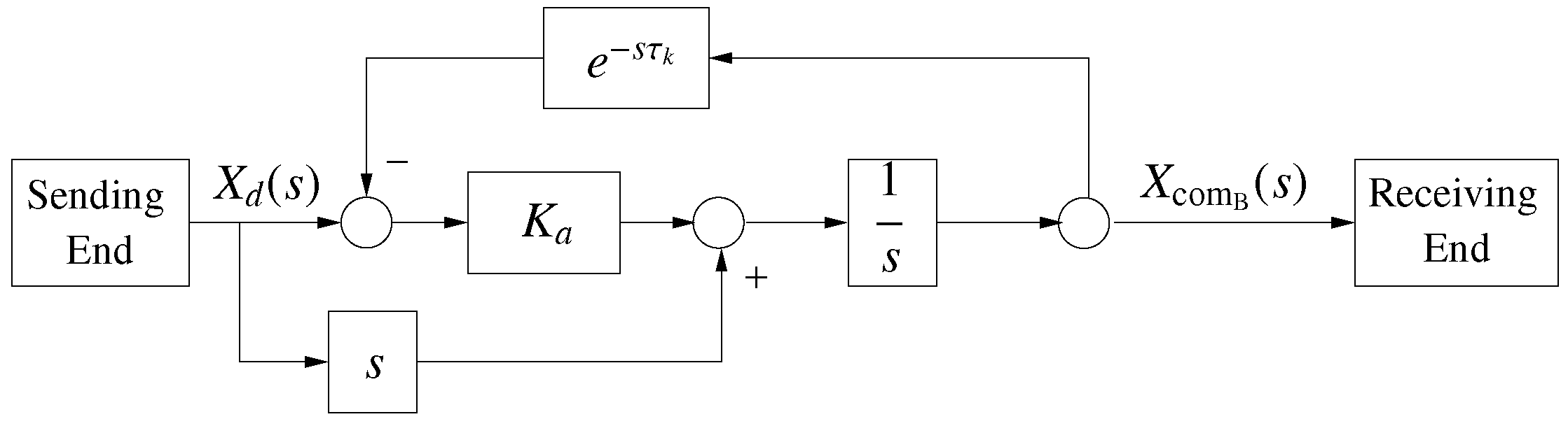
2.3. Predictor-Based Delay Compensation

The predictor-based delay compensation is given by:
x ˙ com B ( t ) = x ˙ d ( t ) + K a x d ( t ) x com B ( t τ ) .
For the constant delay case, Zheng et al., [9] proved that, to ensure the convergence of the predictor error, the compensation gain K a should be within the range:
0 < K a τ < π 2 .
Similarly, for the time-varying delay case, one can use:
0 < K a τ ¯ < π 2 ,
where τ ¯ is the mean value or, alternatively, the maximum value of the time-varying delay. However, since the above inequality is often too conservative, especially in the case of time-varying delays, it is preferable to verify the convergence of the predictor-based compensation of time-varying delays through numerical tests.

2.4. Power System Model with Inclusion of Delay Compensation

If the delay-compensation technique is applied to a power system, the delayed variables x ( t τ i ) in Equation (3) are replaced by the compensated variables. Thus, the standard form for the small-signal model of the power system implemented with the proposed delay compensation is a Neutral Time-Delay System (NTDS). The derivative terms that appear in the delay-compensation methods, namely Equations (4) and (6), lead to the following formulation:
x ˙ ( t ) = F x ( t ) , y ( t ) , x d ( t ) , y d ( t ) , x ˙ d ( t ) 0 m = G x ( t ) , y ( t ) , x d ( t ) , y d ( t ) , x ˙ d ( t ) ,
where F : R 3 n + 2 m R n are the differential equations and G : R 3 n + 2 m R m are the algebraic equations. We refer to this system as the compensated system. We state the following Theorem:
Theorem 1.
We the consider system in Equation (1), in which we apply a derivative control based delay-compensation technique. The system that appears has the form of Equation (7), which is a NTDS. Following a small disturbance into the compensated system, a necessary and sufficient condition for the equilibrium solution to be asymptotically stable is that the real parts of all roots of the determinant of Δ ( λ ) are negative, where Δ ( λ ) is given by:
Δ ( λ ) = λ I p A 0 e λ τ A 1 k = 2 e λ k τ A k ,
where F F , G G for x ˙ d ( t ) = y ˜ d ( t ) , and
A 0 = F x + F y A , A 1 = F x d + F y d A + F y D , A k = E C k 2 D , k 2 ,
with
A = F y 1 F x , B = F y 1 F x d , C = F y 1 F y d , D = B + C A , E = F y C + F y d .
The series in Equation (8) converges if ρ ( C ) < 1 , where ρ ( · ) is the spectral radius of the eigenvalues of a matrix.
The proof can be found in the Appendix A.
Remark 1.
The matrix function in Equation (8) is the characteristic matrix [31]. I p is the identity matrix of order p. The solutions of Equation (A3) are called the characteristic roots or spectrum.
Remark 2.
If the series in Equation (8) converges, the critical eigenvalues that have the largest real parts can be obtained through a Chebyshev discretization method, as described in [13].

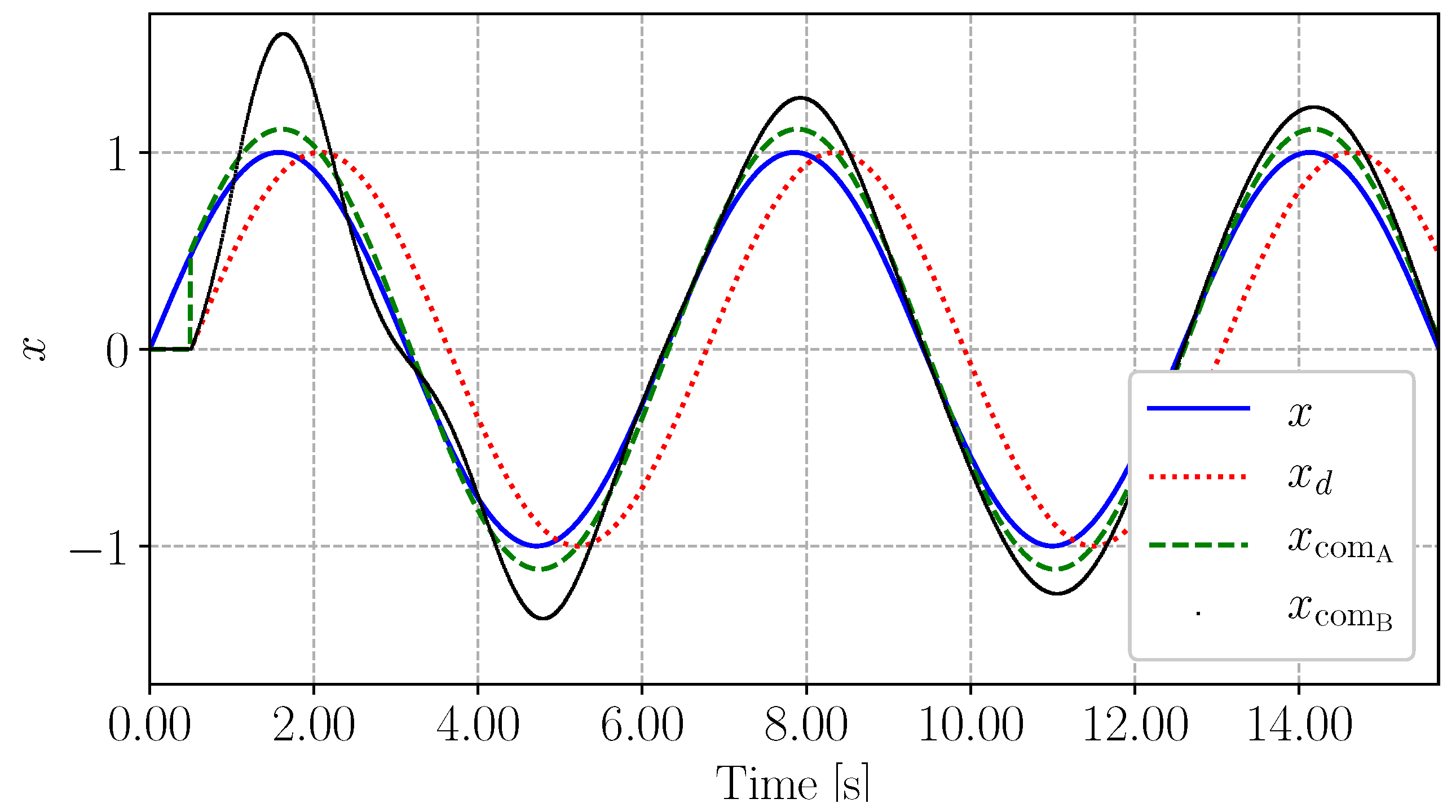
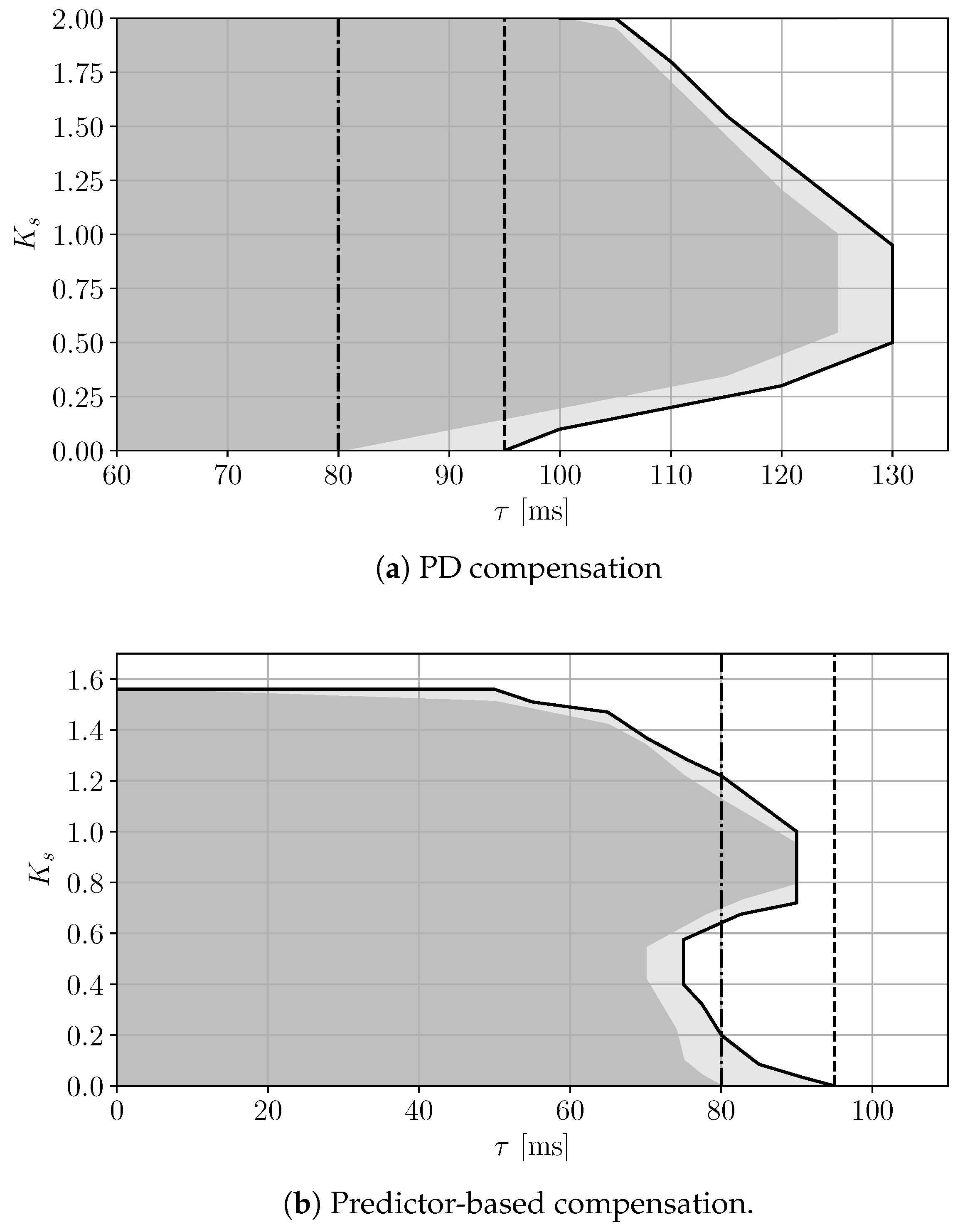
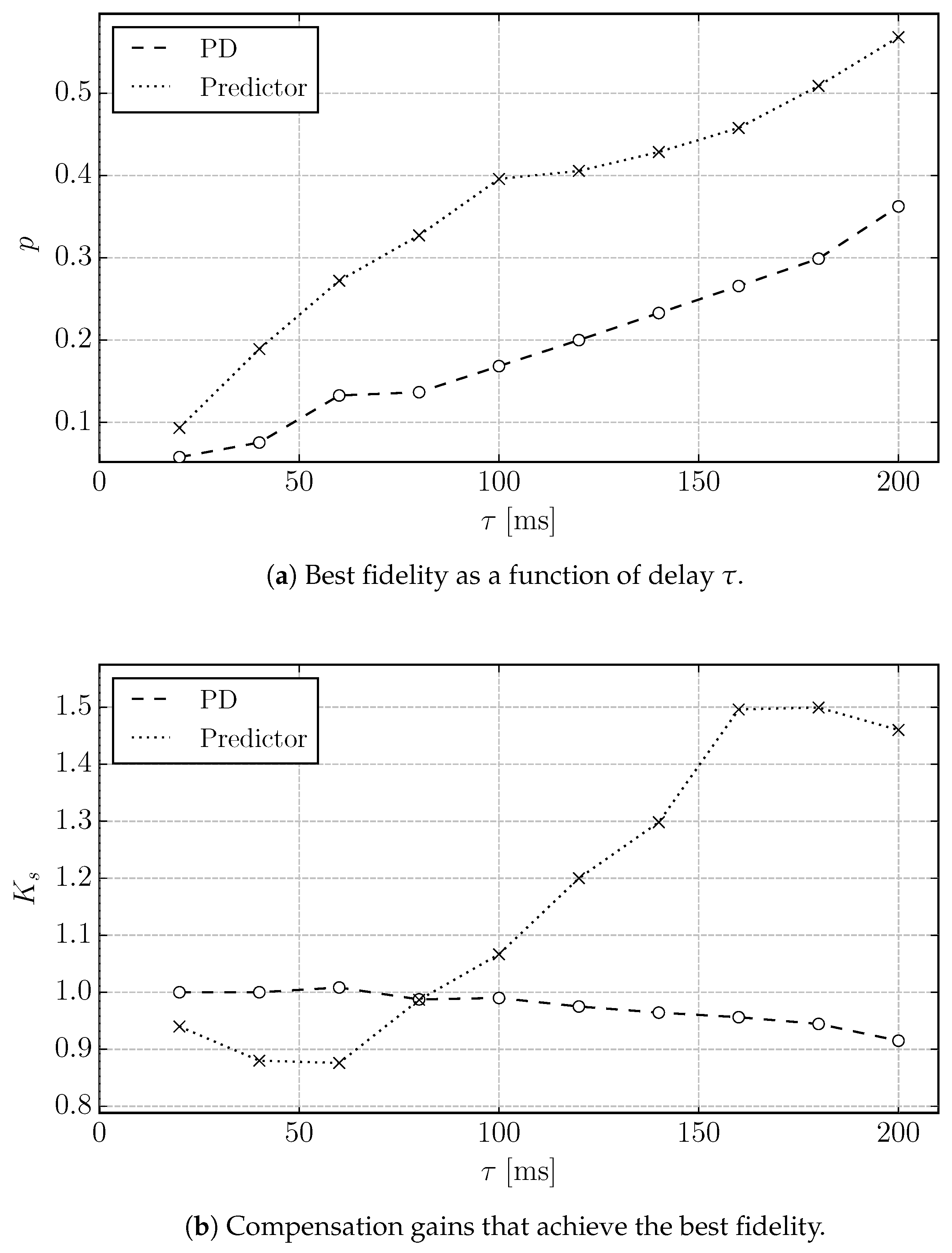
3. Fidelity Comparison

This section discusses the effect of the PD and predictor delay compensation methods on the fidelity of a received signal. To quantify the fidelity improvement, Zheng et al., [9] established a normalized performance index p, as follows:
p = | | x com x | | 2 | | x d x | | 2 .
If p < 1 , the compensation improves the fidelity of the received signal. The smaller is the value of p, the more accurate is the compensation effect.

Illustrative Example

To illustrate and compare the fidelity of Equations (4) and (6), let us consider the following simple signal:
x ( t ) = 0 , if t < 0 sin ( t ) , if t 0 x d ( t ) = x ( t τ ) ,
with τ = 0.5 s.
According to the discussions in Section 2.2 and Section 2.3, we consider the following range of the compensation gains: K τ [ 0 , 1 ] and K a [ 0 , 3.14 ] . Figure 2 shows the variations of the performance index p computed based on the received signals in [ τ , 5 π ] s as the compensation gain varies. The PD-based method provides the best performance for K τ = 0.50 , with a corresponding performance index p = 0.2588 . The predictor-based method shows the best performance for K a = 2.59 , with a performance index p = 0.4942 . Figure 3 shows the trajectories of the compensated signals obtained with the methods, for K τ = 0.50 and K a = 2.59 , respectively.
Figure 3 shows that both methods effectively compensate the phase lag induced by the time-delay. However, they introduce small errors on the amplitudes of the periodic signal. These small errors can be fixed through higher-order compensation [7], the study of which, however, is out of the scope of the paper. The PD compensation achieves a relatively smaller amplitude error and, thus, a better fidelity, especially during the first swing.

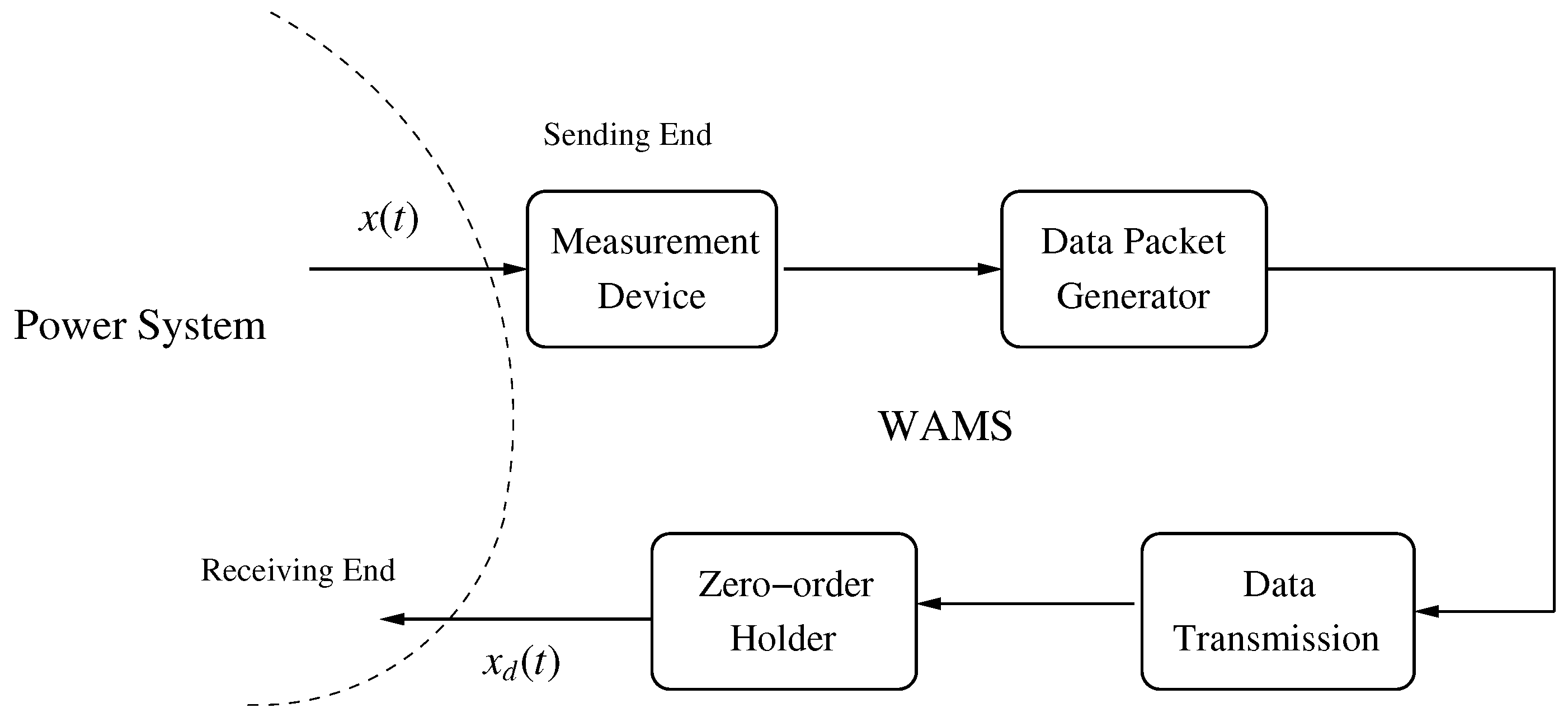
4. Wide-Area Measurement Delay Compensation

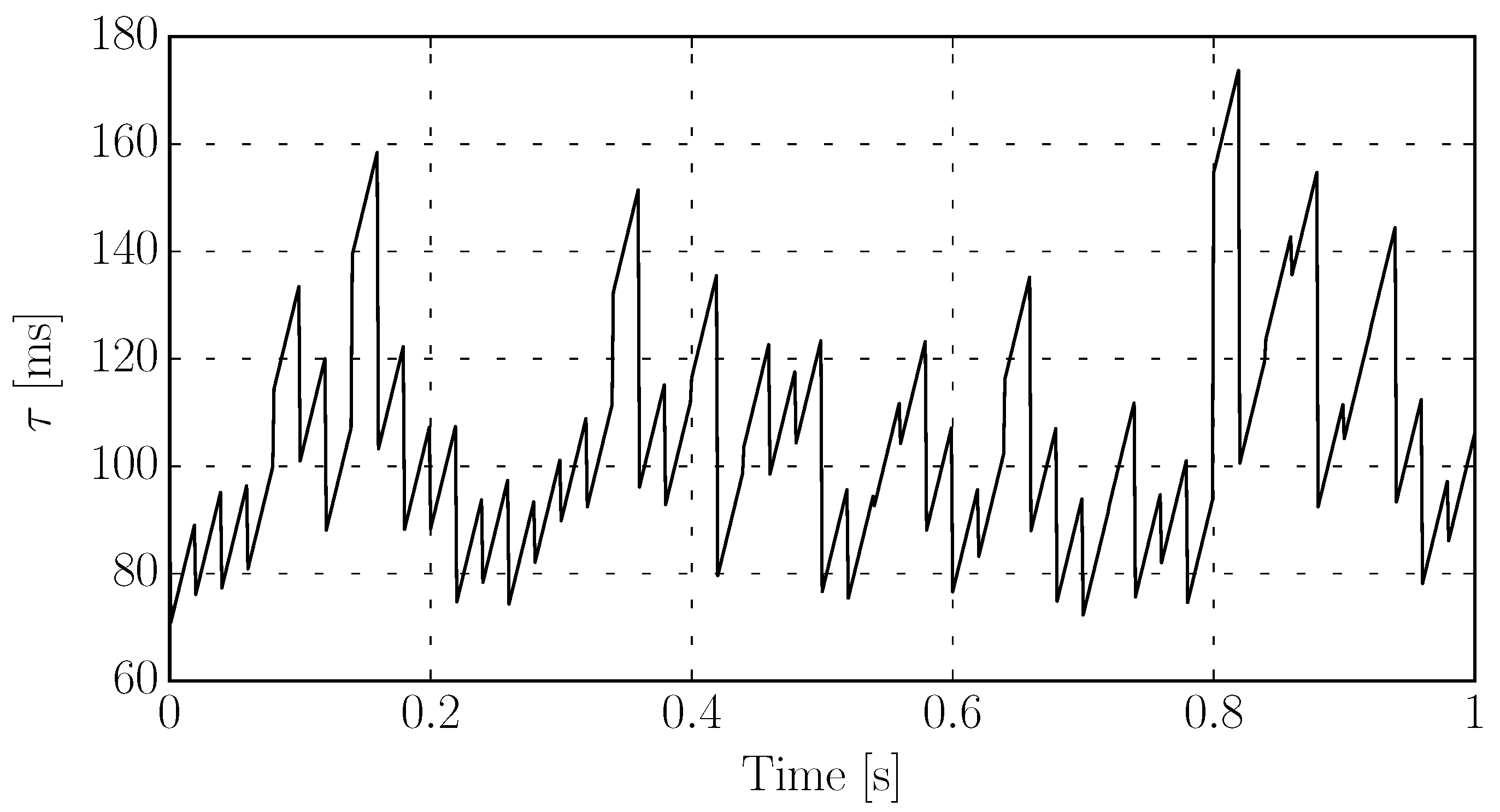
4.1. Wide-Area Measurement Delay Model

Figure 4 shows a time-varying WAMS delay model according to the wide-area communication process discussed in [19].
The signal x ( t ) , which we assume to be a state variable of the DDAE system defined in Equation (1), is collected at a given sampling rate and digitized as data packets. Each packet is then transmitted through a communication network and processed through a zero-order holder (ZOH), which helps to avoid dynamic issues resulting from the possibility that the data packet is lost. Latency arises during this process. The resulting signal at the receiving end can be presented as x ( t τ ( t ) ) . Although the communication process in Figure 4 is digitized, appropriate modeling of the time-varying delay τ ( t ) allows treating the WAMS-based control loop as a part of the continuous model. Under some simplifying assumptions, a time-varying WAMS delay τ ( t ) can be modeled as follows:
τ ( t ) = τ o + τ s ( t ) + τ p ( t ) ,
where τ o is the constant delay for each data packet; τ s ( t ) is a stochastic function that results from network-induced noise and uncertainties, as well as the probability of a data packet loss; and τ p ( t ) is a quasi-periodic sawtooth function that is equal to the time past the receiving of the latest data packet.
Figure 5 shows the time dependency of a typical WAMS delay. In this example, τ o = 70 ms; τ s is Gamma distributed with scale factor a = 10 ms and shape factor b = 2 ; and τ p has a period T = 20 ms and dropout rate c = 10 % . The mean value of the WAMS delay τ ( t ) is:
τ ¯ = τ o + a b 1 c + T 2 ( 1 c ) 2 = 104.57 ms .
Replacing in the characteristic matrix in Equation (A3) the constant delay τ with the time-varying delay in Equation (11) yields:
Δ ( λ ) = λ I n A 0 k = 1 e λ k τ o h p ( λ ) h s ( λ ) A k ,
where
h p ( λ ) = 1 c T λ 1 + ( c 1 ) e λ T 1 c e λ T , h s ( λ ) = 1 + a 1 c λ b .
The critical eigenvalues of Equation (13), however, need to be determined with an iterative technique [19]. The accuracy of the resulting critical eigenvalues heavily relies on the choice of the initial guess for λ .

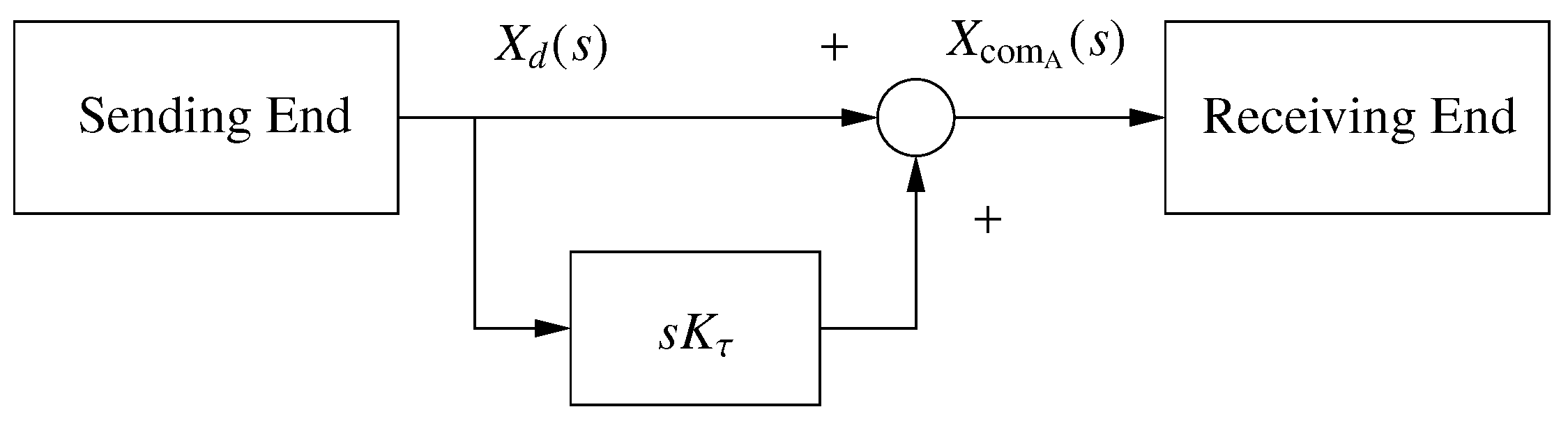
4.2. Implementation of the Delay Compensation

For clarity, the schemes of the PD and predictor-based compensation are shown in Figure 6 and Figure 7, respectively.
Both compensation methods require the first derivative of the delayed signal. As discussed in Section 4.1, the transmission of a signal in WAMS is digitized. Assuming that a data packet arrives at time t k , before receiving the next packet at t k + 1 , the first derivative of the delayed signal utilized by the compensation methods can be set as:
x ˙ ( t ) x ( t k ) x ( t k 1 ) t k t k 1 , t [ t k , t k + 1 ] .
The predictor-based delay compensation also includes a feedback on the predictor error with delay τ k . In general, such a delay is different for each received data packet and its magnitude can be obtained from the time stamp of the data packet itself [25].

5. Case Study

This section provides a thorough comparison of the performances of the PD and predictor-based compensation methods in power system applications. Section 5.1 focuses on the stability impact of the two methods on the IEEE 14-bus system. Section 5.2 studies the best fidelity that the compensation methods can achieve and their effect on the inter-area oscillation modes of the New England 39-bus system.
All simulations in this section were obtained using the Python-based software tool dome [35]. The dome version utilized here was based on Fedora Linux 25, Python 3.6.2, cvxopt 1.1.9, klu 1.3.8, and magma 2.2.0. The hardware consisted of two 20-core 2.2 GHz Intel Xeon CPU s, which were utilized for matrix factorization and Monte-Carlo time-domain simulations; and one nvidia Tesla K80 gpu, which was utilized for the small-signal stability analysis.

5.1. IEEE 14-Bus System

In this section, the IEEE 14-bus system model serves to illustrate the stability impact of the derivative term of the two compensation methods discussed in Section 2. The static and dynamic data of this system can be found in [36]. The system includes one Power System Stabilizer (PSS), which is fed by the rotor speed error of the synchronous machine connected at bus 1. The system with the PSS, and without inclusion of any delay, is stable. The most poorly damped complex pair of eigenvalues has damping ratio ξ = 9.37 % .

5.1.1. Constant Delay

Assume a constant delay τ introduced in the input signal of the PSS. The stability delay margin of the 14-bus system is τ = 95 ms, and the delay margin for which the damping ratio is ξ 5 % is τ = 80 ms. To depict the effect of the delay compensation, the small-signal stability maps of τ against the compensation gains are shown in Figure 8, where K s is a unified quantity to normalize the compensation gains for different values of τ . For PD compensation,
K s = K τ τ ,
and, for predictor-based compensation,
K s = K a τ .
The stability maps are obtained by carrying out small-signal stability analysis 30 × 50 times, in the intervals τ ( 0 , 150 ] ms; K s [ 0 , 2 ] for PD; and K s [ 0 , 1.6 ] for predictor-based compensation.
Figure 8 shows the effect of the two methods. The PD appears to work better than the predictor-based compensation for the 14-bus system. In particular, with a proper gain, the PD increases the small-signal stability delay margin from 90 ms to 130 ms. On the other hand, the predictor-based compensation cannot provide any improvement of the stability delay margin. The delay margin of damping ratio ξ > 5 % is increased from 80 ms to 95 ms by the PD and to 90 ms by the predictor-based compensation.

5.1.2. WAMS Delay

Let us now assume that the control input signal of the PSS is obtained from a WAMS that introduces the time-varying delay shown in Figure 5. In this scenario, the IEEE 14-bus system is unstable, since the rightmost pair of eigenvalues is 0.2053 ± j 11.1262 .
Table 1 shows the rightmost eigenvalues of the IEEE 14-bus system with inclusion of WAMS delay and delay compensation. In this table, a reference quantity K m is utilized to present the value of the compensation gain, which is a referring maximum value of the compensation according to the discussions in Section 2 K m = 2 τ ¯ = 0.2 for PD; K m = π 2 τ ¯ = 15 for predictor-based compensation. According to Table 1, the PD can stabilize the time-varying delay system with K τ [ 0.6 K m , K m ] . In addition, the damping ratio of all eigenvalues of the system with PD compensation and K τ = 0.8 K m is ξ > 5 % . On the other hand, similar to the results obtained for the constant delay scenario, the predictor-based compensation is not effective in stabilizing the time-varying delay system.

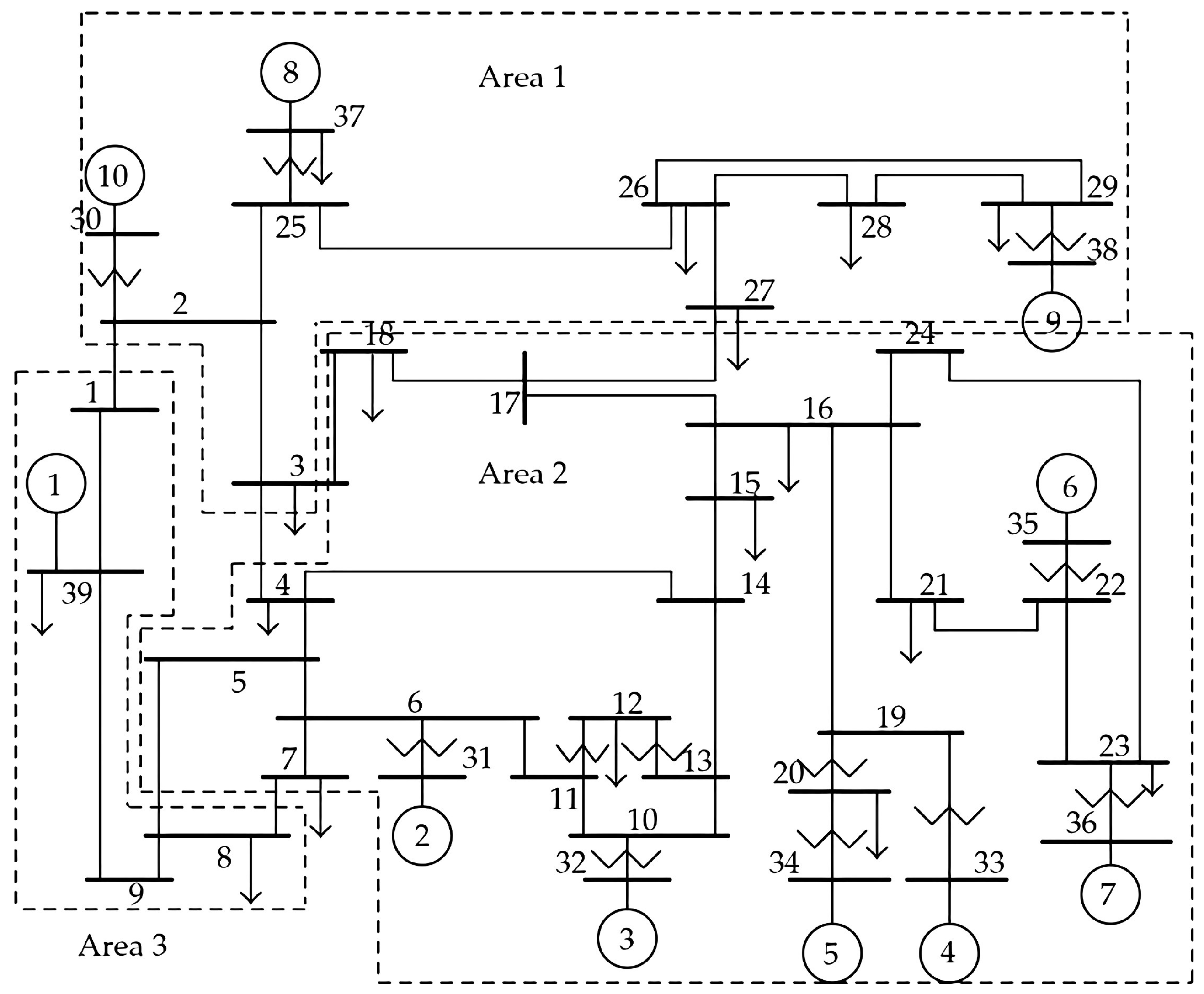
5.2. New England System

This section further discusses the dynamic response of the two delay compensation methods through the New England 39-bus 10-machine system. The static and dynamic data of this system can be found in [37]. The system has been divided into three areas, as shown in Figure 9. Each area includes a PSS, at bus 39, 32, and 35, respectively, to damp the inter-area oscillations. The dynamic behaviors of the 39-bus system shown in the rest of this section are following the N 1 contingency line 1–2 outage.

5.2.1. Constant Delay

Assume that the output signal of the PMU introduces a constant delay τ before arriving at a control center. Figure 10 shows the best fidelity that the compensation methods can achieve and their corresponding compensation gains against different values of τ . Figure 10 was obtained through 10 × 40 time domain simulations for τ ( 0 , 200 ] ms and K s [ 0 , 1.6 ] . The performance index p was computed based on the trajectories of the signals from τ to 49 s after the contingency.
Figure 10 shows that both compensation methods effectively improve the fidelity of the delayed signal for τ [ 0 , 200 ] ms. The PD achieves better fidelity than the predictor-based compensation. Another advantage of the PD, as shown in Figure 10b, is that the optimal compensation gain is always around the fixed quantity K s = 1 for different scenarios, while the optimal gain of the predictor-based compensation varies for different scenarios. Thus, in real-world applications, tuning of the parameters of the PD is easier than that required by the predictor-based method.

5.2.2. WAMS Delay

Let us assume that the measurements are obtained through a WAMS and that the signals are affected by time-varying delays, as shown in Figure 5. In this scenario, time domain simulation results show that the the smallest fidelity of the PD ( p = 0.37 ) is obtained for K τ = 0.095 . The predictor-based compensation achieves the best fidelity ( p = 0.4 ) for K a = 12.5 . Following the line outage, the trajectories of the original, delayed, and compensated signals that yield their best fidelity, are shown in Figure 11. Both methods are able to compensate the phase lag introduced by the delayed signal, but the predictor-based compensation performs slightly worse than the PD, especially during the first swings.
Finally, we consider the scenario where the delayed signal from the PMU feeds the PSS of the generator connected to bus 39. Figure 12 shows the trajectory of the rotor speed of synchronous machine 1 with different input signals of the PSS. Results indicate that the time-varying WAMS delay deteriorates the dynamic oscillations following the contingency. The PD compensation with K τ = 0.095 and the predictor-based compensation with K a = 12.5 , respectively, yield the best overall dynamic performance and effectively fully compensate the communication delay.

6. Conclusions

This paper demonstrates that a derivative term can effectively compensate communication delays of wide-area controllers of power systems. To this aim, the time-domain and eigenvalue analysis methods are utilized to evaluate the effect of the proposed delay compensation methods. The case study provides thorough comparisons of the dynamic behavior of the PD as well as the predictor-based compensation on power system applications. The PD performs better than the predictor-based compensation, according to the scenarios considered in the case study.
These results show that the predictive compensation performs worse than the PD during the first swing of the signal following a contingency. In power systems, the first one or two seconds, i.e., the first swing, following a contingency are the most critical part of the transient and a poor dynamic response in the first swing can deteriorate the whole transient behavior of the system. Controllers that are most effective during the first swing are thus to be preferred. It is important to note, however, that these results do not imply that the PD compensation is always better than the predictor one. In fact, there exist dynamic systems for which the predictive compensation works better than the PD compensation. However, this is not the case of the scenarios considered in the paper. These scenarios represent, as far as we appreciate and based on several tests, typical power systems applications.
Future work will focus on higher-order derivative compensation methods and on validating the proposed compensation methods on hardware-in-the-loop tests.

Author Contributions

All authors equally contributed to this work. All authors have read and agreed to the published version of the manuscript.

Funding

This work was supported by: Science Foundation Ireland, by funding Muyang Liu, Ioannis Dassios, Georgios Tzounas, and Federico Milano under Grant No. SFI/15/IA/3074.

Conflicts of Interest

The authors declare no conflict of interest.

Appendix A

This appendix provides the proof of Theorem 1.
Proof. 
The derivative terms that appear in the delay-compensation methods, i.e., Equations (4) and (6), lead to the formulation in Equation (7). Due to the presence of the independent variables x ˙ d ( t ) , Equation (7) is an NTDS. By introducing the extra equations:
0 n = y ˜ ( t ) x ˙ ( t ) ,
which also means that x ˙ d ( t ) = y ˜ d ( t ) , the NTDS can be transformed into DDAEs in the form of Equation (1). Then, one has:
F ( x , y , x d , y d , x ˙ d ) = F ( x , y , x d , y d , y ˜ d ) G ( x , y , x d , y d , x ˙ d ) = G ( x , y , x d , y d , y ˜ d ) ,
and
F ( x , y , x d , y d , y ˜ d ) F ( x , x d , y ^ , y ^ d ) G ( x , y , x d , y d , y ˜ d ) G ( x , x d , y ^ , y ^ d ) ,
where y ^ = ( y , y ˜ ) . Hence,
x ˙ = F ( x , x d , y ^ , y ^ d ) 0 m + n = G ( x , x d , y ^ , y ^ d ) ,
where F : R 4 n + 2 m R n ; G : R 4 n + 2 m R m + n ; and x R n , y ^ R m + n . Finally, we obtain the following linearized system:
Δ x ˙ = F x Δ x + F x d Δ x d + F y ^ Δ y ^ + F y ^ d Δ y ^ d 0 m + n = G x Δ x + G x d Δ x d + G y ^ Δ y ^ + G y ^ d Δ y ^ d .
The small-signal stability of Equation (7) can be defined through the critical right-most eigenvalues of the pencil of the linearized system in Equation (A1). The fourth and second authors [32] showed that the linearized system in Equation (A1) can be written in the following form of DDEs with multiple delays:
Δ x ˙ = A 0 Δ x + A 1 Δ x d + k = 2 [ A k Δ x ( t k τ ) ] ,
where A k , k = 0 , 1 , 2 , , are given by:
A 0 = F x + F y A , A 1 = F x d + F y d A + F y D , A k = E C k 2 D , k 2 ,
and
A = F y 1 F x , B = F y 1 F x d , C = F y 1 F y d , D = B + C A , E = F y C + F y d .
Assuming the delay τ is constant, the roots of the determinant of Δ ( λ ) are the solutions of
det Δ ( λ ) = 0 ,
where Δ ( λ ) is given by Equation (8). The system is stable at the given point if and only if all the eigenvalues of Equation (8) have strictly negative real-parts. For asymptotic stable states, we have that Re ( λ ) < 0 , or, equivalently, since τ > 0 , τ Re ( λ ) < 0 . Then,
| e τ [ Re ( λ ) + i Im ( λ ) ] | < | e i τ Im ( λ ) | ,
or, equivalently,
| e τ λ | < 1 .
The matrix series in Equation (8) can be written as:
k = 2 e λ k τ C k 1 D = k = 1 [ e λ ( k + 1 ) τ C k ] D .
Hence, the matrix series k = 2 e λ k τ C k 1 D converges if and only if k = 1 e λ ( k + 1 ) τ C k converges. By applying the D’Alembert criterion, k = 1 e λ ( k + 1 ) τ C k converges if:
lim k + e λ ( k + 2 ) τ C k + 1 e λ ( k + 1 ) τ C k < 1 ,
or, equivalently,
| e λ τ | lim k + C k + 1 C k < 1 ,
by using C k + 1 C k C we get:
| e λ τ | lim k + C k + 1 C k | e λ τ | lim k + C k C C k < 1 ,
or, equivalently,
C < | e λ τ | < 1 ,
or, equivalently,
C < 1 .
Hence, the matrix series k = 2 e λ k τ C k 1 D in Equation (8) converges if ρ ( C ) = < 1 holds. □

References

  1. Zhang, Y.; Bose, A. Design of wide-area damping controllers for interarea oscillations. IEEE Trans. Power Syst. 2008, 23, 1136–1143. [Google Scholar] [CrossRef]
  2. Mokhtari, M.; Aminifar, F.; Nazarpour, D.; Golshannavaz, S. Wide-area power oscillation damping with a fuzzy controller compensating the continuous communication delays. IEEE Trans. Power Syst. 2013, 28, 1997–2005. [Google Scholar] [CrossRef]
  3. Milano, F.; Ortega, Á.; Conejo, A.J. Model-agnostic linear estimation of generator rotor speeds based on phasor measurement units. IEEE Trans. Power Syst. 2018, 33, 7258–7268. [Google Scholar]
  4. Zhao, L.; Abur, A. Multi area state estimation using synchronized phasor measurements. IEEE Trans. Power Syst. 2005, 20, 611–617. [Google Scholar] [CrossRef]
  5. Zhu, L.; Lu, C.; Dong, Z.Y.; Hong, C. Imbalance learning machine-based power system short-term voltage stability assessment. IEEE Trans. Ind. Inform. 2017, 13, 2533–2543. [Google Scholar] [CrossRef]
  6. Yu, J.J.Q.; Lam, A.Y.S.; Hill, D.J.; Li, V.O.K. Delay aware intelligent transient stability assessment system. IEEE Access 2017, 5, 17230–17239. [Google Scholar] [CrossRef] [Green Version]
  7. Tian, Y.C.; Levy, D. Compensation for control packet dropout in networked control systems. Inf. Sci. 2008, 178, 1263–1278. [Google Scholar] [CrossRef] [Green Version]
  8. Roy, S.; Patel, A.; Kar, I.N. Analysis and design of a wide-area damping controller for inter-area oscillation with artificially induced time delay. IEEE Trans. Smart Grid 2019, 10, 3654–3663. [Google Scholar] [CrossRef]
  9. Zheng, Y.; Brudnak, M.J.; Jayakumar, P.; Stein, J.L.; Ersal, T. A predictor-based framework for delay compensation in networked closed-loop systems. IEEE/ASME Trans. Mechatron. 2018, 23, 2482–2493. [Google Scholar] [CrossRef]
  10. Wang, S.; Meng, X.; Chen, T. Wide-area control of power systems through delayed network communication. IEEE Trans. Power Syst. 2012, 20, 495–503. [Google Scholar]
  11. Naduvathuparambil, B.; Valenti, M.C.; Feliachi, A. Communication delays in wide area measurement systems. In Proceedings of the 34th Southeastern Symposium on System Theory, Huntsville, LA, USA, 19 March 2002; pp. 118–122. [Google Scholar]
  12. Ye, H.; Liu, Y.; Zhang, P. Efficient eigen-analysis for large delayed cyber-physical power system using explicit infinitesimal generator discretization. IEEE Trans. Power Syst. 2016, 31, 2361–2370. [Google Scholar] [CrossRef]
  13. Milano, F.; Anghel, M. Impact of time delays on power system stability. IEEE Trans. Circuits Syst. I Regul. Pap. 2012, 59, 889–900. [Google Scholar] [CrossRef]
  14. Stahlhut, J.W.; Browne, T.J.; Heydt, G.T. Latency viewed as a stochastic process and its impact on wide area power system control signals. IEEE Trans. Power Syst. 2008, 23, 84–91. [Google Scholar] [CrossRef]
  15. Yao, W.; Jiang, L.; Wu, Q.H.; Wen, J.Y.; Cheng, S.J. Delay-dependent stability analysis of the power system with a wide-area damping controller embedded. IEEE Trans. Power Syst. 2011, 26, 233–240. [Google Scholar] [CrossRef]
  16. Papachristodoulou, A.; Peet, M.M.; Niculescu, S. Stability analysis of linear system with time-varying delays: Delay uncertainty and quenching. In Proceedings of the 46th IEEE Conference on Decision and Control, New Orleans, LA, USA, 12–14 December 2007; pp. 2117–2118. [Google Scholar]
  17. Liu, M.; Ortega, Á.; Milano, F. PMU-based Estimation of the Frequency of the Center of Inertia and Generator Rotor Speeds. In Proceedings of the IEEE PES General Meeting, Atlanta, GA, USA, 4–8 August 2019; pp. 1–5. [Google Scholar]
  18. Lu, C.; Zhang, X.; Wang, X.; Han, Y. Mathematical expectation modeling of wide-area controlled power systems with stochastic time delay. IEEE Trans. Smart Grid 2015, 6, 1511–1519. [Google Scholar] [CrossRef]
  19. Liu, M.; Dassios, I.; Tzounas, G.; Milano, F. Stability analysis of power systems with inclusion of realistic-modeling wams delays. IEEE Trans. Power Syst. 2019, 34, 627–636. [Google Scholar] [CrossRef]
  20. Padhy, B.P.; Srivastava, S.C.; Verma, N.K. A wide-area damping controller considering network input and output delays and packet drop. IEEE Trans. Power Syst. 2017, 32, 166–176. [Google Scholar] [CrossRef]
  21. Ghosh, S.; Folly, K.A.; Patel, A. Synchronized versus non-synchronized feedback for speed-based wide-area pss: Effect of time-delay. IEEE Trans. Smart Grid 2018, 9, 3976–3985. [Google Scholar] [CrossRef]
  22. Yao, W.; Jiang, L.; Wen, J.; Wu, Q.; Cheng, S. Wide-area damping controller for power system interarea oscillations: A networked predictive control approach. IEEE Trans. Control Syst. Technol. 2015, 23, 27–36. [Google Scholar] [CrossRef]
  23. Zhao, Y.; Liu, G.; Rees, D. Networked predictive control systems based on the hammerstein model. IEEE Trans. Circuits Syst. II Express Briefs 2008, 55, 469–473. [Google Scholar] [CrossRef]
  24. Yu, X.; Jiang, J. Analysis and compensation of delays in ff h1 fieldbus control loop using model predictive control. IEEE Trans. Instrum. Meas. 2014, 63, 2432–2446. [Google Scholar] [CrossRef]
  25. Chaudhuri, N.R.; Ray, S.; Majumder, R.; Chaudhuri, B. A new approach to continuous latency compensation with adaptive phasor power oscillation damping controller (pod). IEEE Trans. Power Syst. 2010, 25, 939–946. [Google Scholar] [CrossRef]
  26. Sarkar, T.K.; Ji, Z.; Kim, K.; Medouri, A.; Salazar-Palma, M. A survey of various propagation models for mobile communication. IEEE Antennas Propag. Mag. 2003, 45, 51–82. [Google Scholar] [CrossRef] [Green Version]
  27. Huang, Z.; Schneider, K.; Nieplocha, J. Feasibility studies of applying kalman filter techniques to power system dynamic state estimation. In Proceedings of the 2007 International Power Engineering Conference (IPEC 2007), Singapore, 3–6 December 2007; pp. 376–382. [Google Scholar]
  28. Zhou, N.; Meng, D.; Lu, S. Estimation of the dynamic states of synchronous machines using an extended particle filter. IEEE Trans. Power Syst. 2013, 28, 4152–4161. [Google Scholar] [CrossRef]
  29. Zhao, J. Dynamic state estimation with model uncertainties using h extended kalman filter. IEEE Trans. Power Syst. 2018, 33, 1099–1100. [Google Scholar] [CrossRef]
  30. Liu, Y.; Liu, Y.; Zhang, Y.; Guo, J.; Zhou, D. Wide Area Monitoring through Synchrophasor Measurement. In Smart Grid Handbook; Liu, C., McArthur, S., Lee, S., Eds.; Wiley: Hoboken, NJ, USA, 2016; pp. 1–18. [Google Scholar]
  31. Michiels, W.; Niculescu, S.I. Time-delay systems of neutral type. In Stability and Stabilization of Time-Delay Systems: An Eigenvalue-based Approach; Society for Industrial and Applied Mathematics: Philadelphia, PA, USA, 2007; pp. 15–31. [Google Scholar]
  32. Milano, F.; Dassios, I. Small-Signal Stability Analysis for Non-Index 1 Hessenberg Form Systems of Delay Differential-Algebraic Equations. IEEE Trans. Circuits Syst. I Regul. Pap. 2016, 63, 1521–1530. [Google Scholar] [CrossRef]
  33. Liu, M.; Dassios, I.; Milano, F. On the stability analysis of systems of neutral delay differential equations. Circuits Syst. Signal Process. 2019, 38, 1639–1653. [Google Scholar] [CrossRef] [Green Version]
  34. Liu, M.; Tzounas, G.; Milano, F. A model-independent delay compensation method for power systems. In Proceedings of the Milan PowerTech, Milano, Italy, 23–27 June 2019; pp. 1–6. [Google Scholar]
  35. Milano, F. A Python-based software tool for power system analysis. In Proceedings of the IEEE PES General Meeting, Vancouver, BC, Canada, 21–25 July 2013; pp. 1–5. [Google Scholar]
  36. Milano, F. Power System Modeling and Scripting; Springer: London, UK, 2010. [Google Scholar]
  37. Milano, F.; Ortega, Á. Converter-Interfaced Energy Storage Systems: Context, Modelling and Dynamic Analysis; Cambridge University Press: Cambridge, UK, 2019. [Google Scholar]
Figure 1. Implementation of D-based delay compensation methods.
Energies 13 00342 g001
Figure 2. Illustrative Example. Performance index p for t [ τ , 5 π ] s of D-based compensation methods as the compensation gains vary: (top) PD-based compensation; and (bottom) predictor-based compensation.
Energies 13 00342 g002
Figure 3. Illustrative Example. Trajectories of sending (x), delayed ( x d ), PD-based compensated ( x com A ), and predictor-based compensated ( x com B ) signals.
Energies 13 00342 g003
Figure 4. WAMS elements and their interaction with the power system.
Energies 13 00342 g004
Figure 5. Trajectories of a typical WAMS delay within 1 s.
Energies 13 00342 g005
Figure 6. PD delay compensation diagram.
Energies 13 00342 g006
Figure 7. Predictor-based delay compensation diagram.
Energies 13 00342 g007
Figure 8. Stability maps τ K s of delay compensation methods for the IEEE 14-bus system. Shaded regions are stable. Dark shaded regions indicate ξ > 5 % . The dashed and dashed-dotted vertical lines indicate the stability delay margin and the delay margin for ξ > 5 % , respectively, of the system without delay compensation.
Energies 13 00342 g008
Figure 9. New England 39-bus 10-machine three-area system.
Energies 13 00342 g009
Figure 10. Best compensation effects of the PLL at bus 39 with different constant delays for the New England system.
Energies 13 00342 g010
Figure 11. Trajectories of the measured signals of the PMU installed at bus 39 of the New England system.
Energies 13 00342 g011
Figure 12. Trajectories of the rotor speed of the synchronous machine 1 of the New England system.
Energies 13 00342 g012
Table 1. Rightmost eigenvalues of the IEEE 14-bus system with WAMS delay and delay compensation. K m = 2 for the PD and K m = 15 for the predictor-based compensation.
Compensation GainPDPredictor-Based
0.2 K m 0.1030 ± j 11.2144 0.1841 ± j 11.1718
0.4 K m 0.0133 ± j 11.2987 0.1989 ± j 11.1762
0.6 K m 0.1138 ± j 11.4314 0.2285 ± j 11.1854
0.8 K m 0.1328 ± j 0.0343 0.2885 ± j 11.2056
1.0 K m 0.1228 ± j 15.2758 0.3494 ± j 11.2279
1.2 K m 0.0626 ± j 15.5234 0.4736 ± j 11.2796

