1. Introduction
The theory of complex systems and its applications to modeling network behavior and parameters has brought new methodology and interesting concepts in many areas of science [
1]. There are many examples of possible applications [
2,
3,
4,
5,
6]. Power systems are exposed to a wide range of security threats, including cyber-attacks, failures of its different devices and nodes, weather extreme conditions, terrorist attacks, etc. Many countries try to face these threats by applying smart grid technologies. The research made in the last years gave significant results in reducing the risk of potential blackouts [
7]. Nevertheless, serious failures resulting in large-scale blackouts still occur from time to time [
8]. Such extreme events have serious consequences not only for the broadly understood economy, power system integrity, national security, etc. but also should be the basis of a deeper look on the possible conclusions. We believe that the theory of complex systems with its conceptual apparatus is the answer. This is very important, taking into account the possible future plans related to the energetic security and energy independence of different countries of the EU (European Union), for example, the electrical power connection (bridge) between Poland and Lithuania.
In 2004, Poland and Lithuania, as members of the EU started a new program devoted to cooperation in the field of development of energy, energetic security, and safety of region, an increase of competitiveness, and protection of the natural environment. Among these activities, we have the actions of Polish refinery Orlen and also plans of direct connection of the Baltic energy markets (BEMIP). In the field of electrical energy, the most important is a construction of power connection between Poland and Lithuania as a counterweight to the existing electrical connections of Lithuania, Latvia, and Estonia with Russia via IPS/UPS (the wide area synchronous transmission grid of some post-Soviet republics) system. A Polish–Lithuanian company, LitPol Link, was established to carry out preliminary work in the construction of the energy bridge project. The company’s shares were divided between Polish Electrical Networks (pl. Polskie Sieci Energetyczne, PSE) and Litgrid AB. This step is toward the guarantee of Central Europe’s electrical energy independence [
9].
The quality of the energy supplied is one of the key aspects of a functioning energy system. It is very important not only to deliver power with the best possible quality parameters, such as fluctuations in RMS (root mean square) voltage value, high harmonic content, or frequency fluctuations [
10], but also the continuity and reliability of supply is crucial. SAIDI (
System Average Interruption Duration Index) and SAIFI (
System Average Interruption Frequency Index) parameters [
11] allow to easily measure the stability of the supplied energy, indicating the average time of interruptions in the network operation and the frequency of their occurrence, allowing to assess the quality of the topological structure of connections indirectly.
Breakdowns can be caused not only by atmospheric events but can also be caused intentionally, endangering the safety of the industry. In the long run, the reduced stability of the energy sector leads to a decrease in the attractiveness of the economy for investors [
12].
Properly designed topology of node connections in power networks allows increasing the resistance of the net to damages caused by intentional and random events [
13]. The power grid is an ordered pair of sets
S = {
D, C}, where
D is a set of devices and
C a set of mutual relations between these devices, in other words, a set of configurations. The configuration is an unambiguously defined state of the system structure containing current switches off and on. The current configuration can also be represented as a graph
G = {
V, E} containing nodes
V and edges
E. The typical approach to determining the state of the network is defined by the KDM and EPC (the formats for recording short-circuit data in power networks, commonly used in Poland) standards for writing power flow data [
14].
PSE, the Polish National System Operator, is responsible for the reliability of connections on the highest-voltage lines and on some high-voltage lines, while individual Distribution System Operators (DSO) are responsible for the remaining high-, medium-, and low-voltage lines, whose task is to supply electricity to final customers within the power region. The basis of the policy of electricity supply security is to react as quickly as possible to changes in the system parameters in order to maintain energy quality [
15]. Having in mind that the power grid can be modeled as a graph
G, in this paper, we focus on possible applications of complex systems and networks theory in modeling power network vulnerability. We will focus only on high-voltage lines and nodes related to DSO Rzeszów in the south-eastern part of Poland.
In this paper, the representation of a real electrical (110 kV) network as a graph of nodes and edges is shown. The topological parameters of the network are analyzed. We assume that this real net has some of the features that are omnipresent in complex networks. Usually, such networks consist of many more nodes and are mostly related to social and media relations, but remembering that power network ensures constant electrical energy transport (flow), the importance of such networks is at least at the same level as others. There aren’t many case studies where the parameters of power networks are shown in terms of complex systems, but having in mind that nowadays the distinction between the energy producer and the energy consumer is very difficult (we have a presumption) the features of real power grid can be (and should be) represented in terms of complex networks features and some calculated parameters will allow to describe not only topological parameters of this network but also have a real physical meaning and can be used for analysis of network stability, consistency, and support protection of network safety. We calculated several topological parameters that describe a real electrical network and show that this network can be seen in terms of complex networks. Our analysis is based on the removal of some network nodes (for instance, this can be understood as their failure), and the significant changes appeared in the whole network topology. They lead to a drop in network efficiency and, in turn, to the increase of the energy transmission cost.
The rest of the paper is organized as follows: the short introduction to complex systems apparatus and the concept of complex networks is given in
Section 2. The analysis of case study and source data based on Network Workbench (made by Katy Börner, Alessandro Vespignani, Albert-László Barabási, Indiana University, Bloomington, IN, USA), NetworkX (Aric Hagberg and others, Los Alamos National Laboratory), and Gephi software (initially written by students of University of Technology of Compiègne, The Gephi consortium) packages is given in
Section 3.
Section 4 shows conclusions and the paper summary.
2. Complex Network Model and Power Grid
The concept of complex systems has its roots dated back to the ‘80s of the 20th century. This concept is based on the general systems theory (GST) proposed in the ‘30s of the 20th century by von Bertalanffy [
16,
17] and lately developed by Klir [
18]. Usually [
19] the term system
S is understood as a being
B consisting of
n elements
E = {
e1, e2, …, en}, each element poses
m attributes
A = {
a1, a2, …, am} and between elements there are
k possible different long- or short-range relations
R = {
r1, r2, …, rk},
S = B(
E, A, R). Typically, the definition of complex systems is based on Aristotle’s rule:
the whole is more than the sum of its parts, but there are some taxonomies that precise this general definition and explain some important details [
20].
Complex systems pose many interesting features that can be described in spatial and temporal domains [
21]. In the spatial domain, one of the possible pieces of evidence of complexity in the system are the complex networks. Modelling such networks is usually based on an abstracted graph
G = {V, E} containing
n nodes (vertices
V = {
v1, v2, …, vn}) connected by
m edges
E = {
e1, e2, …, em}. The graph topology can be described as an
n × n adjacency matrix
A = {
aij}, where every
aij element is 1 (if nodes
i and
j are connected by the edge) or 0 (if vertices
i and
j are not connected). Graph
G can be seen as weighted (between each node
i and
j, there is a number
ℓij) or unweighted. In the second case, we are only interested in the fact that there is or no connection, whereas the first case stands for additional information about graph edges: weights
ℓij can represent, e.g., physical distances, cost of transport, communication time, the velocity of the chemical reaction, edge throughput. The second case is a special first-case having
ℓij = 1, ∀
i ≠ j. For every two nodes in the graph, one can calculate the shortest path length
dij as the smallest sum of the
ℓij between all the possible paths in the graph between
i and
j,
dij ≥ ℓij, ∀
i ≠ j. We can also define the efficiency
εij = 1 /
dij, ∀
i ≠ j. If
dij =
∞, then
εij = 0.
The short paths between
i and
j nodes mean high efficiency, and over the whole graph, it can be defined as [
22]:
Given the Equation (1), where
dij is the shortest path between nodes
i and
j, it is easy to calculate the average efficiency of the whole network. There are two types of network efficiency: global and local. Global one (defined by Equation (1)) refers to the entire network, but for each vertex
i there is a possibility to define the local efficiency
Eloc(
Gi), which is the average efficiency of the local subgraphs and shows the fault tolerance of the system; it also indicates the efficient communication between the first neighbors of node
i when
i is removed [
22]. It can also be reflected in the cost of the entire network, as well as, the cost of energy transmission. If the efficiency falls, then the cost rises (for example: in transporting information).
The existence of connections between the nearest neighbors of a vertex i can be described by the clustering coefficient
C. Suppose that a vertex in the network has
ki edges that connect this vertex to other
ki nodes. All of these nodes are node
i neighbors [
14]
The clustering coefficient
Ci of node
i is then defined as the ratio between the number
Ei of edges that exist among these
ki nodes and the total possible number of node connections [
14]
Going further, the clustering coefficient of a vertex can be defined as the ratio of 3-cliques in which this vertex participates. The clustering coefficient value for the whole network is the average of
Ci over all
i [
14].
The distance between two vertices in a network is the number of edges between them in the shortest path. The maximum of all shortest path lengths is the network diameter. The average path length
ℓ can be used to measure the scattering of the network [
23].
Many complex networks seem to be characterized by the so-called small-world property. Even with a large network size, there is often quite a short path between any two vertices. In complex networks, the average shortest paths between two vertices scales as the logarithm of the number of vertices [
23].
For a totally random network, the distribution of node degrees (having direct connection with
k vertices) is described by the Poisson’s distribution [
24]; however, many studies [
24,
25,
26] in recent years indicate that in some random networks, this is moving away from the classic Poisson’s distribution in favor of the power law distributions, which can be described as:
Networks described with power-law distributions are called scale-free networks because they can’t be described in any characteristic scale [
8]; however, this phenomenon is visible only for networks having a sufficient number of nodes. It is stated in [
21] that removing some nodes from the graph will cause cascading consequences, because of the network weakening, but after some time, the system will evolve to a stable state. In the worst-case scenario, the failure of real nodes in the power grid can trigger the whole network cascading outages [
21,
27]. The wide-area blackouts occur frequently, more than one would expect, and these failures are random and independent. According to United States government reports, the number of blackout accidents has not decreased significantly since 1965, despite the fact that many improvements have been made to the electrical power network [
14]. Looking at the problem from the side of complex networks gives a new opportunity to study the possible behavior of the network [
13,
28].
3. Case Study
In this Section, the power grid (110 kV) data obtained from the DSO for Rzeszów and its surroundings (
Figure 1) have been entered into the Gephi software package in the form of a graph. Each network node in
Figure 1 represents a separate vertex of the graph (
Figure 2). The connections between nodes have been redrawn in the form of graph edges, which means that the network of graph connections is the same as the real layout of the transmission network. The created graph (
Figure 2) has 102 vertices and 117 edges. The average vertex degree of the original graph is 2.27, and the average efficiency of the graph is
E(
G) = 0.18. The average value of the path length in the graph is
ℓ = 7.66, and its diameter is 20. The vertices degree was calculated basing on the number of edges that are incident to each node. We assume that edges haven’t got the direction (are undirected) because energy flow can be bidirectional.
For security reasons, it is not possible to show all details concerning, e.g., location and exact parameters of the network nodes (note again: these are the physical parts of the system located in different parts of the south-eastern part of Poland). The aim of the below-presented simulations of the network behavior is to examine the network’s susceptibility to failures (mostly measured by the average efficiency E(G)) and check its (graph) parameters in emergency situations.
The graph can be analyzed in many ways, for example, in
Figure 2, some rings of a large diameter network can be distinguished, which corresponds to the actual connections in the electricity grid. The rings and related bypasses are a typical solution that increases the electrical network reliability; even if one node with a low degree is not working, there is a possibility to ensure the transport of electrical energy.
Figure 3 shows the graphical analysis of the network (from
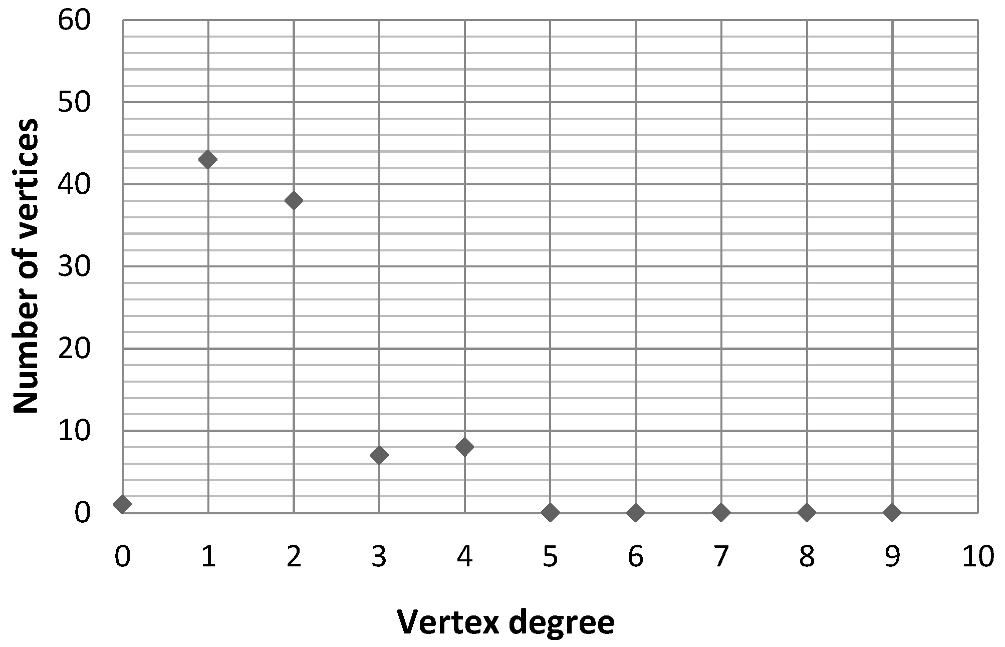
Figure 2) degree centrality. This parameter is the simplest vertices centrality measure; it requires the count of how many connections nodes have—here those numbers are converted into a 0–\–1 scale (the node STW has 1; other node’s centrality is a fraction of its degree). Let’s note that in the case of electrical network node degree shows, taking into account Kirchoff’s law, the number of possible current flows. The bluer the node color, the more important is the node, but there are also more possible current flows ensuring energy supply. The most important nodes are STW, BGC, CHM, RZE, PEL—the names are related to their physical (geographical) localization in the system. These nodes pose the highest degree (the node distribution of the original network is given in
Figure 4) and will be the basis of our carried analysis.
Below we will examine some of the network parameters introducing accidents (nodes failures). The process is carried out basing on the following approach: successive vertices of the graph are removed, starting from the nodes with the highest degrees; after a node removal, when the next one fails, the previous one is not returned to the network. However, because from
Figure 4 it can be seen that there is one node with
k = 9, one node with
k = 6, and three nodes with
k = 5, we decided to create a special scenario for failures appearance (in
Figure 5b a scheme illustrates how to eliminate vertices through the fifth degree through all subsequent stages).
After each removal of the vertex graph properties will be examined. Among them, there are vertex degree distribution, the average vertex degree, the graph density, network efficiency, the clustering coefficient, the average path length, and the graph diameter.
According to the scenario, the first removed vertex will be STW (
k = 9), then BGC (
k = 6), next we have three possibilities: RZE, CHM, and PEL (all with
k = 5). Assuming that nothing distinguishes any vertex with the same degree
k in the network, for three removed vertices (with
k = 5) there are three possible scenarios, for four removed vertices (one node with
k = 5 has been already removed) there are four possible scenarios, and the last one is when there are five removed vertices (
Figure 5).
We assumed that if the node has a high degree it is very important for the whole network (and the system). In the emergency case or during the terrorist attack it can be supposed that such nodes will also be the most exposed. In successive steps, the failures will be related to the nodes colored in red in the diagrams.
Step 1. The first vertex to be removed is the STW (
Figure 6, the red one), which has
k = 9 and this means that its counterpart in the real network has a connection to nine other nodes.
It should be expected that when a high degree node is removed from the network, significant changes can appear in the graph structure.
Figure 7 shows the node degree distribution.
There is a particularly significant decrease (from 50 to 42 nodes) in the number of vertices with degree k = 2 and an increase (from 25 to 30 nodes) in the number of vertices with degree k = 1. This situation is caused by the breaks of the rings in the graph.
The graph lost its consistency, some of its vertices and groups of vertices were separated from its main part (see
Figure 8); however, it can be seen that the majority of the nodes still have any connection to the network; the transport of energy can be ensured. There is still one vertex of the sixth degree and three vertices of the fifth degree. The number of vertices that are not connected to the rest of the network is 11.
Step 2. BGC node is the second most important node in the network, which has connections with six other nodes (see
Figure 8). The nodes degree distribution (
Figure 9) shows a further increase in the number of
k = 1 nodes (now it is 35); the number of nodes with
k = 2, and
k = 3 is almost unchanged. If this node BGC is removed, almost all rings in the graph are separated (
Figure 10a). From
Figure 10b, it can be seen that after this step, the graph was divided into two large subgraphs and several short chains. The number of nodes that are not connected to the majority of the vertices is equal to 49—this is almost half of the number of all network nodes (this is 102). So, after the removal of two nodes, network was divided into two comparable in node numbers subsets. The DSO Centre can apply this information in order to know when the whole network will lose its consistency. It seems to be obvious that the nodes with the highest degree are the most important ones (they ensure the electrical energy transport to many other nodes) in the whole network and the breakdown of any of them can cause serious consequences, but in fact, we were able to show that the breakdown of the only one (STW node—see
Figure 6) can cause graph inconsistency (see
Figure 8 (bottom left part), more than two subgraphs)—this is equivalent to the situation that there is no flow of electrical energy. Even if it is assumed that the STW node is always fully protected and will never breakdown, the breakdown of another node (BGC node—see
Figure 8) will again cause graph inconsistency (see
Figure 10b). The same can be said about the nodes with degree 5 (namely PEL, CHM, RZE). This is the immanent feature of a real net of 110 kV that exists and is managed by one Polish DSO.
Step 3. The analyzed graph (
Figure 2 or
Figure 10a) has 3 vertices of degree 5. In order to obtain reliable results in the form of graph parameters after the elimination of each successive vertex, it was necessary to assume three possible variants (
Figure 5b) of the failure progressing with nodes of
k = 5 degree to conduct several parallel simulations and averaging the obtained results. The elimination of subsequent nodes from the highest through lower degrees requires consideration of more and more cases of failure development. The possible directions of the failure process, as well as the possibility of predicting the damage of a specific nodes are hard to be predicted. In order to make the obtained results credible, simulations were performed in all possible failure paths, and then the obtained results were averaged. For example, when three nodes were removed (
Figure 5b), three paths were possible (one for the node (STW) of the ninth degree, one for node (BGC) of the sixth degree, and three for nodes (RZE, PEL, and CHM) of the fifth degree). The breakdown of the fourth node doubled the number of possible paths of failure/attack on nodes, while the addition of the fifth node is the common end of the development path of failure for the fifth-degree nodes. In total, the number of possible pathways was 6 (1 × 1 × 3 × 2 × 1). The 5th degree vertices are RZE, CHM, and PEL.
Figure 10a shows the location of these vertices in the graph.
Figure 11 shows the graph after the removal of all three vertices with
k = 5 degrees (in total five nodes were removed). These nodes have been eliminated, taking into account all possible combinations (see
Figure 5b, the last step) in order to maintain the reliability of the results. The graph is divided into several unconnected large subnetworks and a few smaller ones. However, if in the next step only the node PEL is removed, the number of nodes connected to the majority of the graph equals the number of disconnected nodes.
It is not difficult to conclude that the further removal of nodes with degree
k = 4 could only be considered theoretically since the actual network (
Figure 11) would be almost completely incapable of any operation.
The scheme and order of the elimination of nodes are illustrated in
Figure 5a,b, while the averaged values from the last stage, along with the rest of the data, are illustrated in the following charts (
Figure 12,
Figure 13 and
Figure 14).
With the removal of subsequent nodes, the distribution of degrees of vertices has changed—at the beginning the dominant group was the vertices of degree 2 (many chains as a part of rings), and after the last stage of the removal, the dominant group are the vertices of degree 1. This means that they are connected by only one edge with another vertex.
The distribution of degrees (
Figure 14) of vertices in the graph after the last stage of the simulation (when the nodes STW, BGC, RZE, CHM, PEL were removed) has changed significantly compared to the original state of the network (
Figure 4).
The maximum degree of the vertex is 4, which is a significant difference compared to the original value of 9.
The changes of graph parameters (average vertex degree, graph density, network efficiency, clustering coefficient, average path length, graph diameter) calculated during the analysis are presented in
Figure 15,
Figure 16,
Figure 17,
Figure 18,
Figure 19,
Figure 20.
The average degree of the vertex of the graph decreased after the removal of five nodes with the highest degree. This was a linear decrease (
Figure 15). Very similar observations were recorded at the graph density coefficient (
Figure 16).
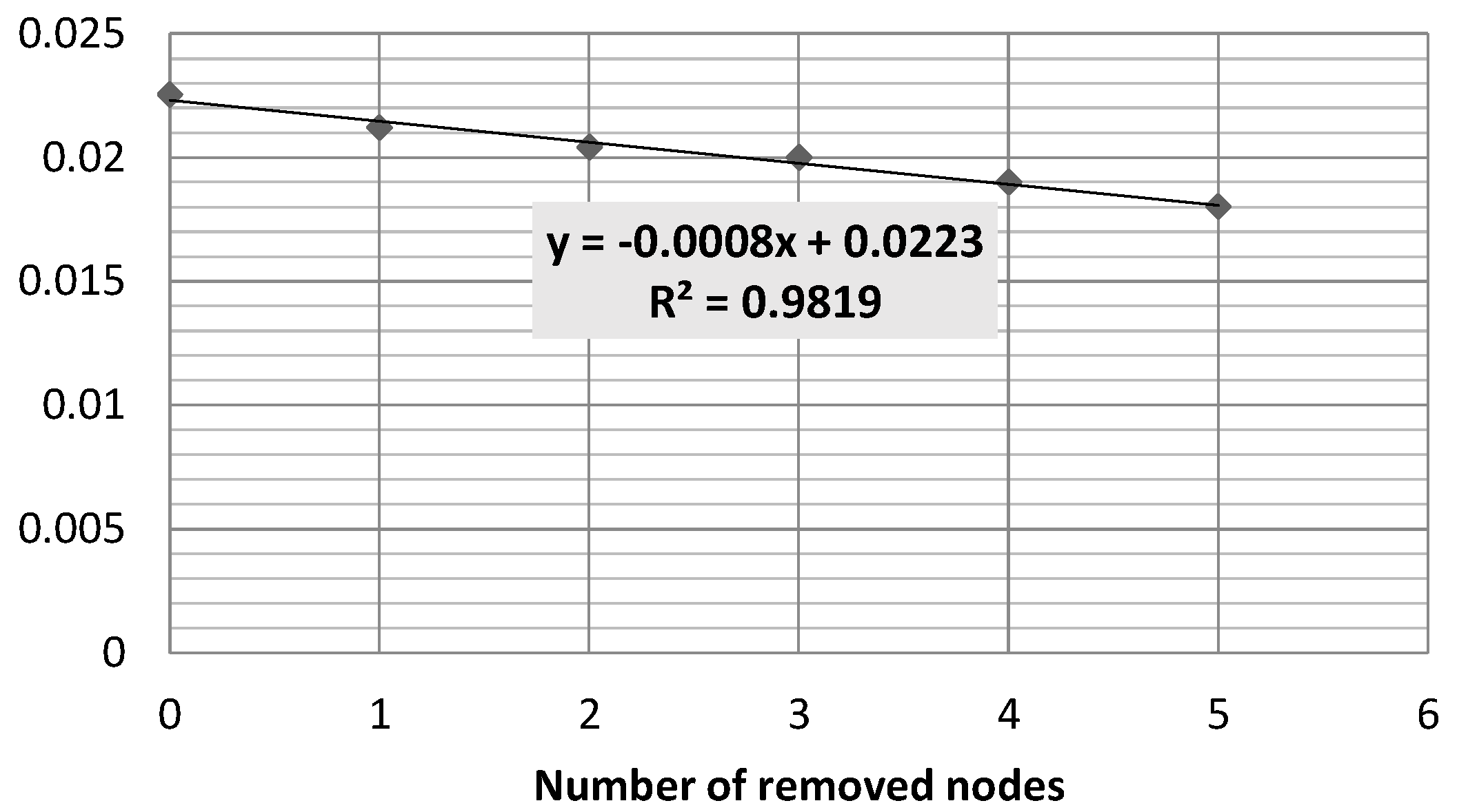
The value of the network efficiency parameter (
Figure 17—it is given in log-lin scale) decreased very rapidly when the first nodes were removed. The graph has become less concentrated, which is also confirmed by the decrease in the clustering coefficient value (
Figure 18).
The observed changes (
Figure 17) are represented by a semi-power law. We have focused only on the core of the network (lines of high voltages, 110 kV); therefore, it is not possible to indicate the existence of the (expected) power law, but let’s note that removing only five nodes caused the decrease of the network efficiency from 0.182 to 0.048 (almost four times, see
Table 1).
Remembering that at the beginning the average value of the path length in the graph was
ℓ = 7.66 it can be seen that after removal of node STW, it increased to 9.14 and finally fell to 5.643 (see
Table 1,
Figure 20). The network diameter at the beginning was 20, then it increased to 25 (removal of STW node) and established a value 17 (
Figure 21). The clustering coefficient of the graph (
Figure 19) decreased the most after removing the first vertex and after removing each vertex of the fifth degree.
In the analyzed case both values decreased in relation to the initial value (primary form of the network) except for the state after the removal of the first (and most important) node with the most connections.
The meaning of the parameters calculated in
Table 1 is as follows:
The number of nodes and edges in the graph corresponds to the physical number of objects in the transmission network (here, the nodes understood as transformers, power distribution stations, and the edges understood as transmission lines).
The average vertex degree is the average number of connections (edges, 110 kV power lines) per node—does not have to be high for network security, as opposed to graph density and clustering coefficient.
The graph density shows the ratio between the number of existing edges and the number of all possible edges in the graph. In dense graphs, this ratio is close to 1 and corresponds to a high number of redundant backup connections (bypasses). These connections are costly for DSO, but they protect against the loss of connections and separation of nodes from the main part of the network.
The average clustering coefficient parameter for node i was defined by Equations (2) and (3) and for the whole graph is calculated as an average of the overall graph node. As with graph density, the clustering coefficient also translates to certain extent into the number of network redundancies.
The
local (per node) and
average efficiency parameters describe the physical efficiency of the system as it was written in
Section 2 and can be calculated by Equation (2).
The average path length and graph diameter describe the physical properties of the system. The first one is defined by Equation (4), whereas the second one represents the highest of the shortest path between each pair of vertices in the graph. The higher the values of these parameters, the more geographically extensive is the system; simulations of the most important node failures reduce these values because it divides the network into smaller and independent parts, however, they cannot be able to ensure energy transport (they are disconnected from the main graph).


