Sliding Mode Control for Micro Turbojet Engine Using Turbofan Power Ratio as Control Law

Abstract

The interest in turbojet engines was emerging in the past years due to their simplicity. The purpose of this article is to investigate sliding mode control (SMC) for a micro turbojet engine based on an unconventional compound thermodynamic parameter called Turbofan Power Ratio (TPR) and prove its advantage over traditional linear methods and thrust parameters. Based on previous research by the authors, TPR can be applied to single stream turbojet engines as it varies proportionally to thrust, thus it is suitable as control law. The turbojet is modeled by a linear, parameter-varying structure, and variable structure sliding mode control has been selected to control the system, as it offers excellent disturbance rejection and provides robustness against discrepancies between mathematical model and real plant as well. Both model and control system have been created in MATLAB^® Simulink^®, data from real measurement have been taken to evaluate control system performance. The same assessment is conducted with conventional Proportional-Integral-Derivative (PID) controllers and showed the superiority of SMC, furthermore TPR computation using turbine discharge temperature was proven. Based on the results of the simulation, a controller layout is proposed and its feasibility is investigated. The utilization of TPR results in more accurate thrust output, meanwhile it allows better insight into the thermodynamic process of the engine, hence it carries an additional diagnostic possibility.

1. Introduction

Aviation industry always have to face the challenge of sustainability [1] which permanently inspires researchers to find novel approaches [2,3].

Turbojet engines, even if their utilization has reduced in commercial aviation during the past decades due to their comparably less propulsive efficiency [4], still have a role in different propulsion systems. There is an increasing interest in Unmanned Aerial Vehicles (UAV’s) in the past decade [5], which has led to a considerable interest in developing micro turbojet engines, as stated in [6,7] or [8], because these engines can be applied on military UAV’s, which can include high-speed aircraft (as shown in [9]), where the turbojet already provides fair propulsive efficiency. Meanwhile, there is an ever-increasing interest in radio-controlled model airplanes that imitate real aircraft in civil sector as already reported by [10], and these devices are becoming more attractive [11]. Micro turbojet engines can act as auxiliary power plant of sailplanes, one can find really early initiatives like [12] as well as recent studies presented e.g., [13]. Although the non-optimal speed range of sailplanes turbojets can still be an alternative to piston engines, because they feature relatively simple structure along with reduced weight which is a benefit for small units, as it was stated by [14]. On the other hand, as the aero-thermodynamic processes are similar to large scale engines possibly with bypass, micro turbojet engines can be utilized in research and education as well, as reported by several authors such as [15,16] or [17]. According to [18], results obtained on turbojet engine can be used to draw conclusions about non-propulsion power development units, which further enhances the role of turbojets in research applications. In several cases turbojets form the basis of a different development version like turboprop, as found in [19]. Variable nozzles are already being under investigation for turbofan engines as mentioned in [20], which system can also be assessed on turbojet engines ([21] or [22]).

Control of turbine engines is an inevitable system of the power plant that ensures fast and accurate reaction of the engine on changing demands from the flight crew. They must provide precise regulation of thrust output even if this parameter is traditionally not measurable when the engine is installed. Although there have been investigations into the possibility of thrust measurement during flight reported by [23], the control of turbine engines still depends on rotating speed and EPR.

SMC is one of the important research field in control theory and design of the last decades. It is a kind of Variable Structure Control systems (VSCS) which was evolved by Soviet scientists Emel’yanov and Barbashin in the late 1960s; they have laid the fundamentals of this technology as reported by their articles [24] and respective textbooks [25,26]. Some years later this technology has spread after having been presented to the Western scientific community through textbook written by Itkis [27] and journal article prepared by Utkin [28]. SMC has been developed as a new control design method for a wide range of systems including nonlinear, time-varying, discrete, large-scale, infinite-dimensional, stochastic, and distributed systems as mentioned by [29].

SMC is a nonlinear control method that has proven an effective robust control for modifying the dynamics of nonlinear systems by application of a discontinuous control signal according to [30]. This robust control methodology has been applied to a wide variety of practical systems, such as general industrial applications, e.g., electric power systems including permanent magnet synchronous motors which are favorable in transportation [31], electromechanical [32] and electro-hydraulic systems [33], and robotics including multitude of medical usages like robotic scalpel position control [34] or control for lower limb rehabilitation as well [35]. Furthermore, aerospace controls are also involved, like space manipulators [36], thrust-vector control for spacecraft landing [37] active suppression for combustion instabilities [38], or limit protection control for gas turbine engines [39] as well as setpoint tracking control with output constraints for turbofans [40].

SMC systems are designed to guide the system states onto a particular surface in the state space, named sliding surface. Once the sliding surface is reached, SMC maintains the states on the close neighborhood of the sliding surface. According to Utkin [28] or Ali and Abdulridha [30], there is a two stage controller design:

• First part: implies the design of sliding surface, that the sliding motion satisfies design specifications.
• Second part: concerns the choice of a control law which will make the switching surface attractive for the state of the system.

The aim of this article is to establish sliding mode control (SMC) for single stream micro turbojet engine based on linear, parameter-varying mathematical model using the unconventional Turbofan Power Ratio (TPR) as the basis of the control law.

The novelty of this research lies in the fact that a compound thermodynamic variable, which has originally been utilized on high bypass ratio turbofans for secondary thrust control law, is now investigated, how it can be applied to the control system of turbojet engines as primary thrust parameter. The main hypothesis of the present work is that TPR is applicable to single stream turbojets as the basis of thrust control system because it is proportional to the thrust output. Despite the apparent contradiction between the designation of TPR and the turbojet application, the authors have already proven in [41] that the TPR allows its usage for control of turbojet engines and it has a considerable advantage over conventional rotor speed or Engine Pressure Ratio (EPR) as well.

In this article the authors introduce the steps of the design of a sliding mode controller for a micro turbojet engine with fixed exhaust nozzle which allows reducing the system to a Single-Input-Single-Output (SISO) structure. As a unique feature that must be emphasized, in contrast to conventional control laws that use rotating speed or engine pressure ratio, this control relies on TPR, which is perfectly proportional with thrust, allowing an accurate control. Throughout the paper, in Section 2 the mathematical model of the engine is first introduced, in which Section 2.1 describes the LPV model which is chosen, since there were measurements and identification of the particular engine according to a linear state space representation, which was extended over the entire operating range of the engine. The next step was to design the controller itself, this step is described in Section 2.2. The creation of a simulation in MATLAB ^® Simulink^® is detailed in Section 3, by splitting into a theoretical background in Section 3.1 and the description of the simulation itself in Section 3.2. The comparison of simulation and other control laws is performed in Section 3.3, comparison of SMC with conventional PID control is accomplished in Section 3.4. The results, including comparison of simulation and measurement data from the turbojet, are presented in Section 4. Using these data, the authors have proven that the control is performing properly through the entire operating range of the engine. Section 5 discusses the results and proposes a buildup for the control system. Finally, in Section 6 the authors provide the conclusion of the performed work and give an outline of future work.

2. Design of SMC for Micro Turbojet Engine

2.1. LPV Model of the Turbojet

The research work was conducted on a PD-60R engine which was converted from turbocharger into turbojet. Figure 1 represents the major aerodynamic stations that play an important role in defining the model of the engine along the longitudinal section that shows the schematic construction of the turbojet. Station 0 is the undisturbed ambient condition, where both pressure and temperature are measured. Station 1 is intake, this location does not include sensors on the particular engine. Compressor inlet and outlet are represented by station 2 and 3, respectively. In these locations the corresponding total pressures $p_{t2}$ and $p_{t3}$ are monitored. Station 4 is turbine inlet, where the non-uniform temperature field does not allow the measurement of turbine entry temperature. Therefore, as it is conventional on other engine types, exhaust gas temperature $T_{t5}$ is measured at the turbine discharge, which is located at station 5. The temperature $T_{t4}$, which is the turbine inlet temperature used hereafter, is not measured, it is computed using $T_{t5}$ and other measured parameters. Finally, jet pipe exhaust is indicated with station 8, but in the particular system this station is not equipped with sensors.

The mathematical model that simulates real plant behavior provides an evaluation of controller and engine cooperation. Models can be based on black-box approach, when the physical details are out of scope and a simplified transfer function of the plant is obtained [42], or they can use physical laws to describe the operation of the plant with more or less details as described in [22,43]. For the present research, an intermediate solution is chosen, which is a linear state-space model with variable parameters to enable accurate simulation through the entire operating range of the engine. The solution is intermediate, since state-space model relies on physical laws described below, but is also simplified into matrices that do not immediately reveal the original physical plant. The LPV model is based on a linear state-space representation of the turbojet, which uses the assumption that the engine comprises of three main storage capabilities that determine the dynamic behavior:

• kinetic energy storage in the rotating assembly, which depends on the rotating speed n;
• heat energy storage in the combustion chamber, that can be described by turbine inlet total temperature $T_{t4}$;
• mass storage in the combustion chamber, which is proportional to the turbine inlet total pressure $p_{t4}$, by converting mass using ideal gas law.

The above mentioned parameters form the main governing equations of the system. The conservation laws lead to the following main correlations (1)–(3) with respect to rotor speed n, turbine inlet total pressure $p_{t4}$ and turbine inlet total temperature $T_{t4}$, respectively. These comprise the state vector x. The main control law is based on $TPR$, which is defined in (4), this parameter is the output y of the system. This formula has been rearranged to reflect the dependence on state variables.

$$\dot{n}=\frac{P_T{\eta }_m-P_C}{\mathsf{\Theta }{\left(\frac{\pi }{30}\right)}^{2}n}$$

(1)

$${\dot{p}}_{t4}=\frac{p_{t4}}{T_{t4}}{\dot{T}}_{t4}+\frac{R_g{T}_{t4}}{V_{CC}}({\dot{m}}_3+{\dot{m}}_{fuel}-{\dot{m}}_4)$$

(2)

$${\dot{T}}_{t4}=\frac{1}{c_v{m}_{CC}}[({\dot{m}}_3{h}_3+{\dot{m}}_{fuel}{H}_a{\eta }_{CC}-{\dot{m}}_4{h}_4)-c_v{T}_{t4}({\dot{m}}_3+{\dot{m}}_{f}uel-{\dot{m}}_4)]$$

(3)

$$TPR=\frac{p_{t3}}{p_{t2}}\sqrt{\frac{T_{t4}}{T_{t2}}}=\frac{p_{t4}}{{\sigma }_{CC}{p}_{t2}}\sqrt{\frac{T_{t4}}{T_{t2}}}=y$$

(4)

Let us consider the conventional linear state-space representation of the above described system, where the partial derivatives, which determine the dynamics of the plant, are considered changing with the operational mode of the engine, thus the modeled object has variable matrices, which yield the system of Equations (5) and (6), as described in textbooks like [44] or [45]. The tilde sign shown over the variables indicates the deviation from a selected nominal operating condition.

$$\dot{\tilde{x}}=A\left(p\right)\tilde{x}+B\left(p\right)\tilde{u}$$

(5)

$$\tilde{y}=C\left(p\right)\tilde{x}+D\left(p\right)\tilde{u}$$

(6)

In [41] the authors have established the mathematical model and have shown an identification that was performed for a single selected nominal operating point. Then, using multiple stable operating points from the same measurement, the entire range has been modeled, where the originally constant matrix members have been replaced by interpolated values determined from the discrete points. The main difference in contrast to conventional LPV models (like [46]) is that the interpolation uses TPR as decision variable.

The normal operating range of the PD-60R is indicated in

Table 1. Main parameters of PD-60R micro turbojet engine.

Operating Condition	n (1/min)	${\pi }_C$ (-)	$T_{t4}$ (K)	TPR (-)
Idle	63,000	1.22	885	2.15
Nominal	113,900	1.97	1015	3.69
Maximal	120,900	2.14	1025	4.03

. Although the original T3 40 trim turbocharger compressor was intended to reach up to 153,400 rpm by the manufacturer Honeywell, due to different bearings, the current speed range is according to Table 1. The measurement included a total of eleven different steady state operating conditions, during which the main parameters have been recorded to provide data for identification.

The measurement for identification was performed between idle and nominal, the main engine parameters are indicated in Figure 2, where the chart starts from the stabilized idle condition, and it shows state variables, command input in percentage, thrust and TPR as well. The latter is scaled by a factor of ten, rotor speed is indicated in thousands of rpm, $T_{t4}$ is divided by ten, and finally $\mathsf{\Delta }{p}_{t4}$ is the gauge pressure at turbine inlet above atmospheric one. The measurement was carried out in multiple steps, thus the engine can sufficiently be stabilized in each different operating mode.

At each stable operating regime the main parameters have been evaluated in order to obtain the matrix members as shown in (7) to (9). Matrix D is excluded as the system does not have a direct feed forward behavior. The equations also indicate the nominal values which are considered as reference values for Figure 3, that correspond to the nominal operating condition indicated in Table 1.

$$\mathbf{A}=\left[\begin{array}{ccc}\frac{\partial \dot{n}}{\partial n}& \frac{\partial \dot{n}}{\partial p_{t4}}& \frac{\partial \dot{n}}{\partial T_{t4}}\\ \frac{\partial {\dot{p}}_{t4}}{\partial n}& \frac{\partial {\dot{p}}_{t4}}{\partial p_{t4}}& \frac{\partial {\dot{p}}_{t4}}{\partial T_{t4}}\\ \frac{\partial {\dot{T}}_{t4}}{\partial n}& \frac{\partial {\dot{T}}_{t4}}{\partial p_{t4}}& \frac{\partial {\dot{T}}_{t4}}{\partial T_{t4}}\end{array}\right]=\left[\begin{array}{ccc}-14.21& 9.376& 102.5\\ 6295& -4393& 52320\\ -15.04& 9.381& -686.5\end{array}\right]$$

(7)

$$\mathbf{B}=\left[\begin{array}{c}\frac{\partial \dot{n}}{\partial {\dot{m}}_{fuel}}=0\\ \frac{\partial p_{t4}}{\partial {\dot{m}}_{fuel}}=\frac{p_{t4}}{m_{CC}}\\ \frac{\partial T_{t4}}{\partial {\dot{m}}_{fuel}}=\frac{H_a{\eta }_{CC}-c_v{T}_{t4}}{c_v{m}_{CC}}\end{array}\right]=\left[\begin{array}{c}0\\ 6.749\\ 1.552\end{array}\right]·{10}^8$$

(8)

$$\mathbf{C}=\left[\begin{array}{c}\frac{\partial TPR}{\partial n}=0\\ \frac{\partial TPR}{\partial p_{t4}}=\frac{1}{{\sigma }_{CC}{p}_{t2}}\sqrt{\frac{T_{t4}}{T_{t2}}}\\ \frac{\partial TPR}{\partial T_{t4}}=\frac{TPR}{2T_{t4}}\end{array}\right]=\left[\begin{array}{c}0\\ 1.879\\ 150.7\end{array}\right]·{10}^{-5}$$

(9)

The different matrix members naturally change throughout the operational envelope of the micro turbojet engine. These changes are covered by an interpolation between individual discrete point values identified via measurement. This method has been based on the description offered by [47]. The different members are indicated in Figure 3, where red lines represent the rotor speed derivatives, green lines stand for the turbine inlet total pressure derivatives, and the turbine inlet total temperature derivatives are shown with blue lines. The input matrix members are magenta, and output matrix parts are drawn with black. The piecewise linear interpolation was practical selection because several parameters show significant variation between neighboring points.

2.2. Sliding Mode Control for Micro Turbojet Engine

As it has been emphasized in previous sections of this article, the novelty of the developed control system is that it utilizes TPR as primary thrust parameter instead of conventional rotor speed or EPR.

The two-step design begins by determining the sliding surface, which is typically defined by the equation shown in (10), as a function of error and error derivative. In (10), the scalar parameter p defines how quickly the controller drives the plant towards the new reference condition. In the present case, the authors have chosen $p=4$, which already provides sufficient rise time as will be discussed in the results part of this article.

$$\sigma =\dot{e}+p·e$$

(10)

The main difference using TPR also inhibits a different calculation of the error and its derivatives. The tracking error is equal to the difference between the actual TPR output of the system and the desired TPR, as shown in (11).

$$e=TP{R}_{act}-TP{R}_{des}=\frac{p_{t4}}{{\sigma }_{CC}{p}_{t2}}\sqrt{\frac{T_{t4}}{T_{t2}}}-TP{R}_{des}$$

(11)

The derivatives of (11) will be used in the calculation of the sliding surface. Even if the desired TPR could be divided into the similar factors like the actual TPR, this change would not make sense, as if the operator of the engine commands higher TPR, it will not act independently on these variables.

The derivative of the turbine and compressor inlet total pressure are defined in the Equations (12) and (13) below. In the present research the turbine inlet pressure is changing due to variations in operating mode of the engine, but the compressor inlet pressure is maintained at a constant value. Later, in further steps of this research the $p_{t2}$ can be subject to changes to represent different flight conditions.

$$\frac{\partial e}{\partial p_{t4}}=\frac{1}{{\sigma }_{CC}{p}_{t2}}\sqrt{\frac{T_{t4}}{T_{t2}}}$$

(12)

$$\frac{\partial e}{\partial p_{t2}}=-\frac{p_{t4}}{{\sigma }_{CC}{\left(p_{t2}\right)}^2}\sqrt{\frac{T_{t4}}{T_{t2}}}$$

(13)

The dependency of the error term e on combustion chamber pressure recovery factor ${\sigma }_{CC}$ is shown by the corresponding derivative as indicated in (14). Typical values for different combustion chamber designs lie around $0.93,\dots ,0.97$, meanwhile the variation of a given type is naturally limited to around $\pm 0.01$ of the nominal value. Hence, this parameter is considered constant in the present step of the research, but according to measurement results, the model should incorporate the possibility to handle this parameter as variable for later developments.

$$\frac{\partial e}{\partial {\sigma }_{CC}}=-\frac{p_{t4}}{{\left({\sigma }_{CC}\right)}^2{p}_{t2}}\sqrt{\frac{T_{t4}}{T_{t2}}}$$

(14)

The derivative of turbine inlet total temperature $T_{t4}$ is shown in (15).

$$\frac{\partial e}{\partial T_{t4}}=\frac{p_{t4}}{2{\sigma }_{CC}{p}_{t2}\sqrt{T_{t4}}\sqrt{T_{t2}}}$$

(15)

The derivative of compressor inlet total temperature $T_{t2}$ can be defined as (16), similarly to $p_{t2}$, it is defined but not used yet, its usage is maintained for future development.

$$\frac{\partial e}{\partial T_{t2}}=-\frac{p_{t4}\sqrt{T_{t4}}}{2{\sigma }_{CC}{p}_{t2}{T}_{t2}\sqrt{T_{t2}}}$$

(16)

The tracking error derivative calculation follows the structure $\frac{\partial e}{\partial x}·\frac{\partial x}{\partial t}$ for all x parameters, which is indicated in (17).

$$\begin{array}{c}\dot{e}=\frac{\sqrt{T_{t4}}}{{\sigma }_{CC}{p}_{t2}\sqrt{T_{t2}}}\frac{\partial p_{t4}}{\partial t}-\frac{p_{t4}\sqrt{T_{t4}}}{{\sigma }_{CC}{\left(p_{t2}\right)}^2\sqrt{T_{t2}}}\frac{\partial p_{t2}}{\partial t}-\frac{p_{t4}\sqrt{T_{t4}}}{{\left({\sigma }_{CC}\right)}^2{p}_{t2}\sqrt{T_{t2}}}\frac{\partial {\sigma }_{CC}}{\partial t}+\hfill \\ \hfill \frac{p_{t4}}{2{\sigma }_{CC}{p}_{t2}\sqrt{T_{t4}}\sqrt{T_{t2}}}\frac{\partial T_{t4}}{\partial t}-\frac{p_{t4}\sqrt{T_{t4}}}{2{\sigma }_{CC}{p}_{t2}{T}_{t2}\sqrt{T_{t2}}}\frac{\partial T_{t2}}{\partial t}\end{array}$$

(17)

The second step is to determine the control input, which results in an action that drives the sliding variable $\sigma$ to zero in a finite time by directing system trajectories onto the sliding surface. The engine is modeled as a SISO structure, the only control input being the ${\dot{m}}_{fuel}$ fuel mass flow rate supplied to the combustion chamber.

A typical problem for SMC systems is the phenomenon of chattering, when the error is close to zero and due to the discontinuous sign function that determines control input, the controller effort changes rapidly between two opposite values. This is disadvantageous for mechanical actuators or other system components, like fuel pump. To overcome this problem, there are multiple solutions, one of which is widely used, which is the use of saturation instead of sign function. The definition is found in (18), where a small, positive number $ϵ$ is introduced into the denominator. If $\sigma$ approaches zero, the saturation smoothens the change of the output.

$$SAT=\frac{\sigma }{\left|\sigma \right|+ϵ}$$

(18)

3. Methods for Simulation of SMC in MATLAB ^® Environment

3.1. Description of the Simulation Software

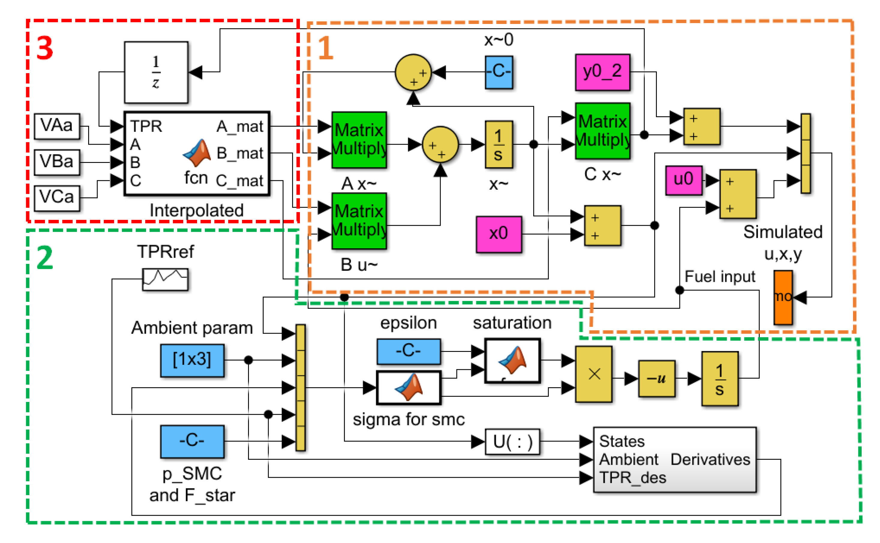
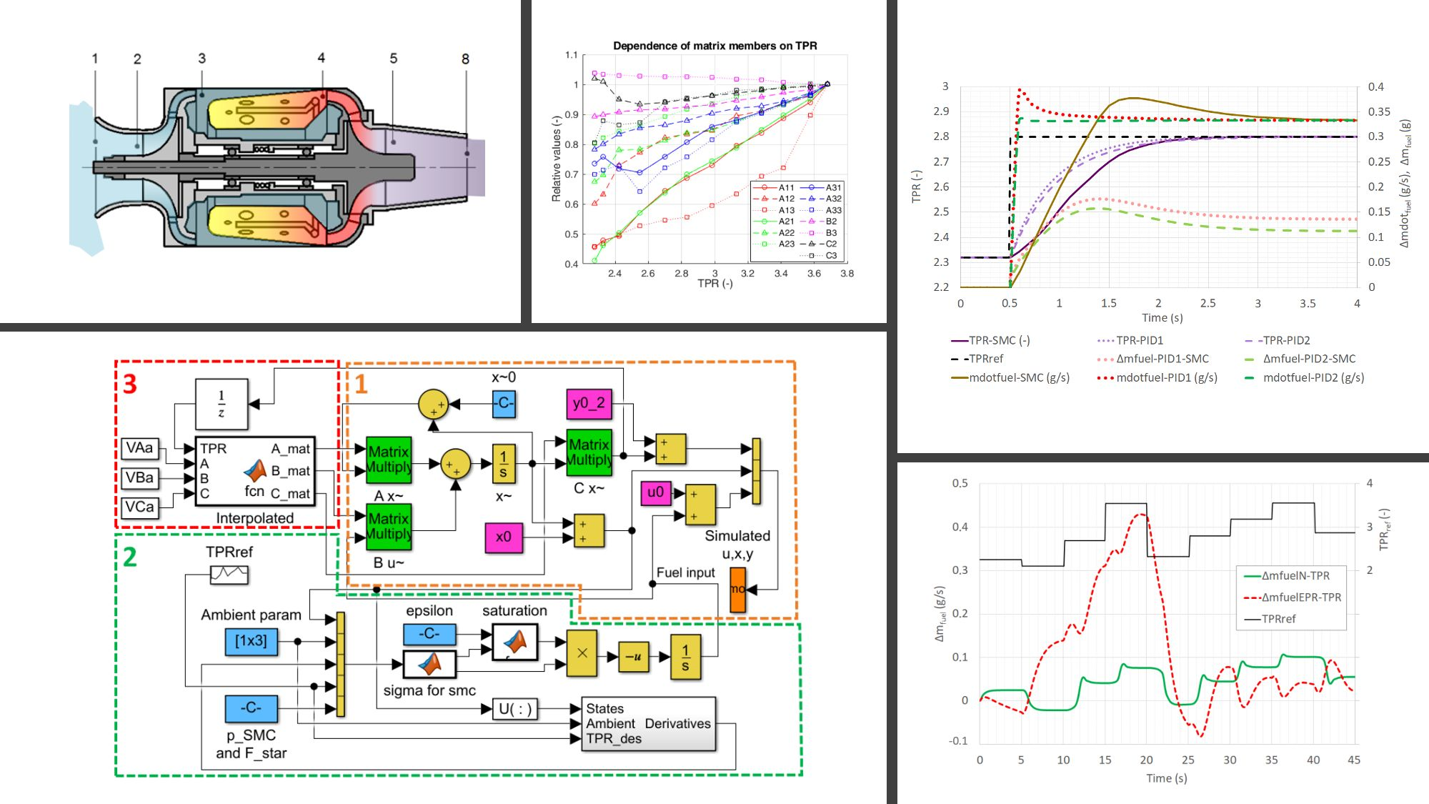
In order to validate the performances of sliding mode control, a set of simulation were performed in Simulink^® version R2018b without using any specific toolboxes, according to the block structure indicated in Figure 4. The purpose of the following simulations is to show the suitability of the proposed approach and its superior performance against a traditional Proportional-Integral-Derivative (PID) based approach. The block diagram consists of three main parts; the first one, which is labeled #1 with orange dashed boundary, represents the state space model which is the basis of this work, the second shows the SMC model and it is indicated with #2 in within green box; meanwhile, the last one #3 defines the LPV decomposition of system matrices and input scheduling, surrounded by red rectangle.

The state space model, indicated by #1 in Figure 4, represents the dynamic behavior of our engine. It comprises the calculation of state variable derivatives using matrices A and B, the calculation of which will be described later; furthermore, it contains standard mathematic operations like addition (circles), vector concatenate (vertical bar) and integration (blocks labeled “1/s”), the latter providing the finite changes due to dynamic behavior of state variables. The light blue box at the center top part includes the initial conditions labeled ${\tilde{x}}_0$, while the three magenta blocks serve for transitioning from deviation model into real physical parameters by defining initial conditions for state vector, input and output. The green boxes represent matrix multiplication, which is the core of the state space model. The orange colored simulated variable output transfers the results into MATLAB workspace for further investigation after the simulation has ended.

The second main block encircled by green borders represents the controller and its related functions. The main part of SMC is found in the center of this block, labeled as “sigma for SMC”. This is a MATLAB function, i.e., it contains the conventionally written program that performs the necessary calculation. On the left side of this entity, one can see a tall vector concatenation, which introduces system states, ambient parameters, derivatives, reference and coefficients p and $F^{*}$ to the main block. The reference TPR block contains a sequence which corresponds to another measurement, in order to make it sure the model can be validated against real operational data. The second MATLAB function in this area is labeled “saturation”, this ensures that the chattering can be eliminated by defining a small, positive value $ϵ$, which is found just left of the parent block in a blue rectangle. The saturation block receives $\sigma$ from sigma calculation, the second output is $F^{*}$, which is multiplied with the output of saturation block, then negation and integration take place. One important input group for the sigma calculation are the derivatives of different variables. The sub-model in the right bottom corner includes discrete time derivation for states, ambient and TPR demand. Values with higher noise components also include discrete-time low-pass filter. These values are then sent to the vector concatenate at the entry of sigma block.

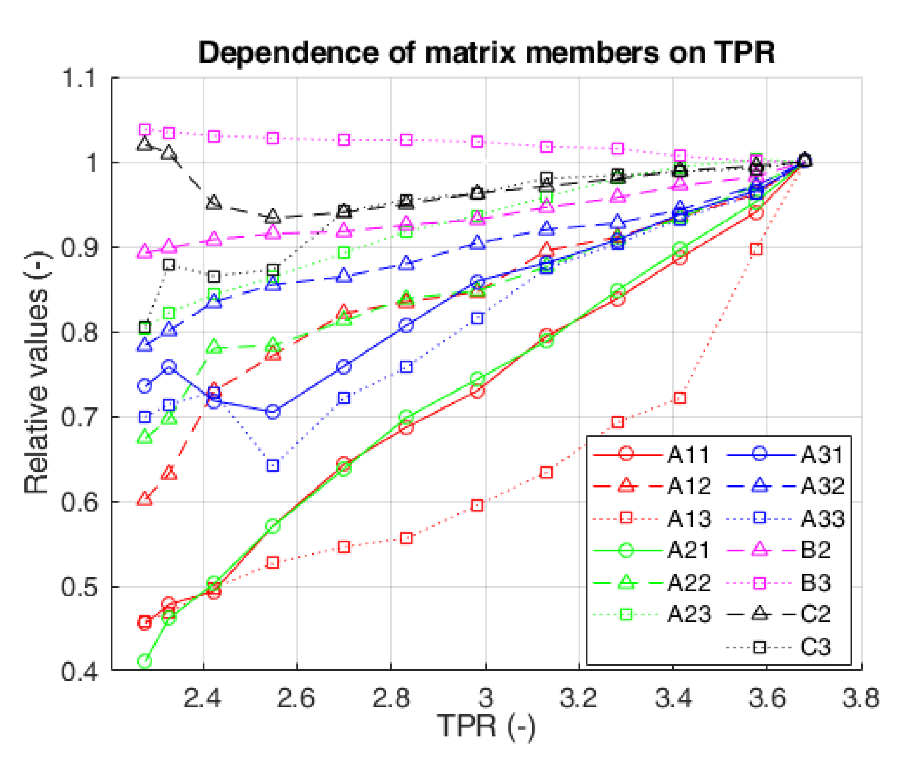
The last group contains the LPV decomposition. This utilizes another MATLAB function, where the label also explains the behavior, i.e., this function provides piecewise linear interpolation between specified operating points. The three input matrices are compound, three-dimensional arrays, where the individual 2D matrices are ‘stacked’ in the third dimension. Each ‘plane’ therefore corresponds to a previously specified (measured) operating condition with a corresponding TPR value. The interpolation will select two neighbors depending on actual TPR, which comes through a unit delay in order to eliminate the algebraic loop in the system.

The simulation has a fixed step setting with the fundamental sample time being $5\times {10}^{-4}$ s. Automatic solver selection has been enabled, but according to the simulations already performed, MATLAB has selected almost exclusively the ode3 Bogacki-Shampine solver.

3.2. Description of the Simulation

The simulation includes three main steps, the first one is comparison to measurement, the second is to provide comparison between SMC for different control parameters TPR, EPR and rotor speed; finally, the third part consists of PID systems to prove the superior performance of SMC itself.

The first simulation was arranged to provide validation with real measured data. For this reason, the main steps in the reference TPR correspond to those values, which were acquired during the engine operation. It must be noted, that the authors have carried out a different measurement for validation, in contrast to the original measurement for identification. The evaluated period of the original measurement took a total of three minutes and ten seconds, but because the simulation does not include noise (i.e., it does not completely simulate real world environment), the simulated parameters will hold a stable value after each transient. Therefore, the transients have been simulated only with sufficient time (5 s) for each to allow all the parameters to approach at their respective values and stabilize. Thus, the simulation was only 45 s, which reduced simulation time and the amount of data generated by the software. In order to match the full length of the measured and simulated time series, the stable values of simulated parameters have been extrapolated.

The range in which different parameters were running throughout the simulation is indicated in

Table 2. Ranges of different engine parameters.

Parameter	Minimum	Maximum
n (×1000 rpm)	71.124	111.8
$p_{t4}$ (kPa)	124.0	183.8
$T_{t4}$ (K)	870	1001
$TPR$ (-)	2.25	3.56
$EPR$ (-)	1.019	1.146

. These values will be important in the later part of the investigation to be set as boundaries for the other assessments.

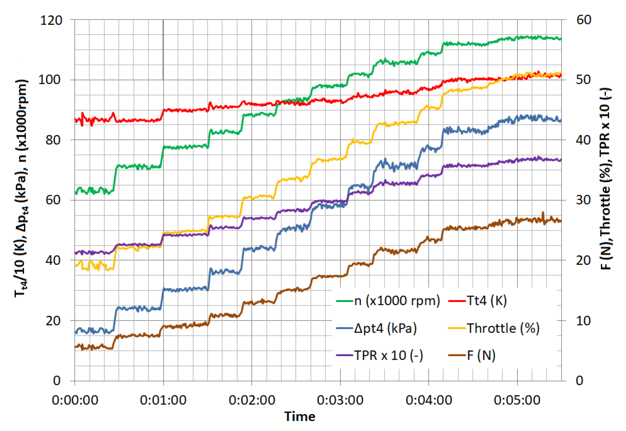
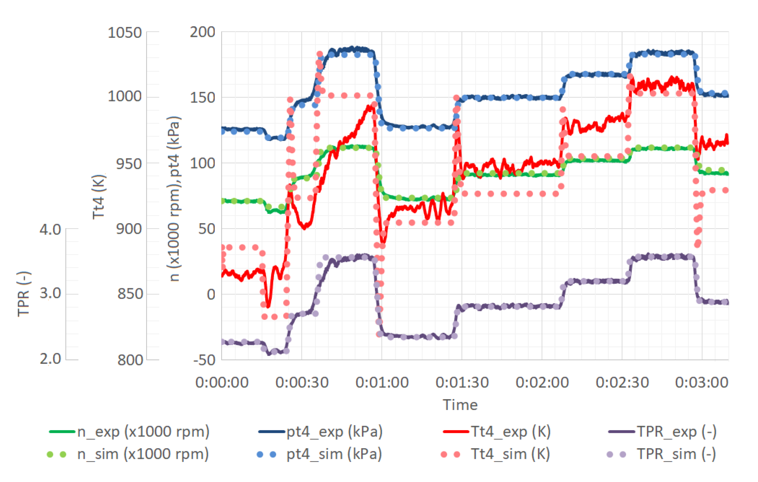
The primary parameters including state variables and TPR are indicated in Figure 5 which shows both measured and simulated values. The formers are indicated by dark solid lines, meanwhile, the latter are shown with lighter dotted series. According to the time series, the majority of the simulated parameters follow the measured data correctly, i.e., the identification can be accepted with the full operating range. There is only one variable, $T_{t4}$, which has lower accuracy, but it is also slightly exaggerated due to the different scale in use. On the other hand, there are multiple explanations for the inability of this parameter to match the corresponding measurement. The error is considered to be introduced by the measurement itself, as the engine has only six evaporation tubes for the fuel injection due to its small size. Therefore, the temperature field is somewhat heterogeneous at turbine inlet and outlet as well. In order to reduce the influence of measurement equipment toward the flow itself, there was only one thermocouple installed to measure the outlet temperature $T_{t5}$ and a calculation based on other thermodynamic parameters yielded the turbine inlet temperature $T_{t4}$. The calculation and derived errors have surely contributed to the increased error levels. In different operating conditions one can see both positive and negative overshoots, however, the trend of the parameter follows the awaited values correctly. As a second founding, one can state that simulation always introduces peaks at the beginning of transient processes. This can be explained as the gas turbine first receives changing fuel injection, then it can react according to the dynamics of the system, that is, the rotor speed can change, which in turn affects the air mass flow rate and the temperature can finally decay.

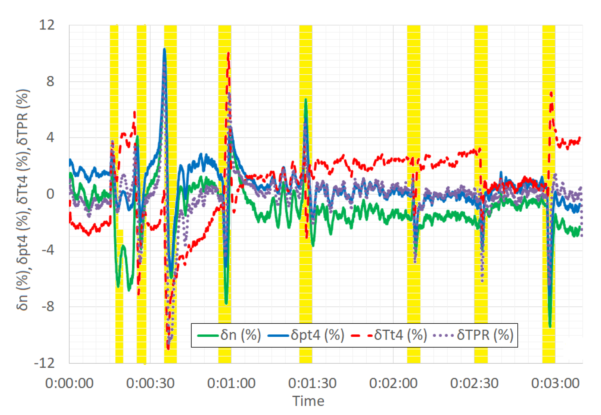
For a more detailed assessment some basic statistical properties must be checked. Firstly, the relative errors of the main parameters throughout the operation can be evaluated based on the information indicated in Figure 6. Every time when the demand is being changed the diagram shows a local peak. This sudden increase in relative errors has basically two main contributing factors, which are described below.

Firstly, the real dynamic behavior of the turbine engine is as follows. Let us consider an acceleration of the turbine to create more thrust. Due to changes in demand, the control system increases fuel supply. At the first moment, this leads to richer mixture in the combustion chamber resulting in increasing turbine inlet temperature $T_{t4}$. As this temperature rises, the available turbine power gets higher, and the rotor speed begins to grow. This leads to a higher amount of air mass flow rate which tends to reduce the temperature, which, on the other hand will be higher than the initial but lower than the peak during the first moment of the transient.

The second reason for the peaks in relative errors is that there is a difference between real fuel supply dynamics and simulation. In the real system the fuel mass flow rate is influenced by the rotating speed of the fuel supply pump. Therefore, it inherently will have a delay due to rotor dynamics. On the contrary, in the simulation, the authors have chosen a simpler way, as the transients themselves were not the most important parts of this investigation, namely, the fuel supply was changed in abrupt steps. Therefore, these peaks, which arise from the different nature of measurement and simulation, are not considered further and are highlighted in Figure 6 with yellow background.

The remaining values are investigated by mean and maximum absolute errors, standard deviation and mean absolute percentage error. Corresponding information for each variable can be found in

Table 3. Error terms of different engine parameters.

Parameter	MAE	MAAE	STD	MAPE (%)
n (×1000 rpm)	1.1703	4.6047	1.4034	1.3240
$p_{t4}$ (kPa)	1.4356	8.3710	1.9154	0.9498
$T_{t4}$ (K)	19.696	54.458	22.191	2.0940
$TPR$ (-)	0.1731	1.4041	0.2457	0.6185

. The majority of the examined parameters exhibit a reasonable match between measurement and simulation, typical absolute percentage errors are lying around or less than 1%. The only variable that has higher errors is turbine inlet total temperature. The absolute error terms seem to be significant, but due to the magnitude of temperature values the percentage error is still not extraordinarily high.

As it was stated above and in Figure 5 and Figure 6 one can see that $T_{t4}$ measured and simulated lines do not match exactly. Nevertheless, the role of $T_{t4}$ in TPR is reduced due to the square root function and the relative magnitude of the errors is not significant compared to absolute value of the variable itself. Therefore, the results can be accepted as the overall relative errors are still not significant, the maximum of mean absolute percentage error is only around 2.1%. Moreover, this phenomenon can definitely be improved by developing the measurement system. This development, however, has not been carried out yet, because the entire system should be redesigned to facilitate measurements under flight conditions. This work surely will require considerable changes to the whole system.

Based on the statement above regarding the acceptable error level, the realized mathematical model is considered to be able to simulate the real engine operation in the normal operating range.

3.3. Comparison of TPR to Other Control Laws

Gas turbine engine control still depends on rotor speed or EPR, as reported by [48], or [49], respectively. In order to prove the control system based on TPR control law has advantages over conventional parameters, the authors have prepared three different simulations which have the same buildup, the only deviation between each other is the control law. The assessment consisted of two independent parts, the first being the comparison of thrust versus the given control law, the second was the comparison using real measurement data.

First of all, the sigma computing block had to be altered, which can be seen near to the center of Figure 4, in order to contain error and derivative computation regarding the actual control variable. Furthermore, the adjustment of the references was necessary. At this point, there is another branch in the investigation due to the different requirements of the intended comparisons. To check thrust correlation with the control parameters, a single slope has been inserted into the Simulink software, replacing the original TPR reference. On the other hand, when time series against real data were to be obtained, the measurement provided the values of the corresponding variable.

Controllers for rotor speed and TPR had same p and $F^{*}$ values, the single difference was in handling the $ϵ$, for rotating speed, due to the much higher magnitude of this parameter, it was set to 2500, instead of the original 0.1 for the TPR. Due to much smaller range of EPR changes, the values of $p_{EPR}$ = 1.5, $F_{EPR}^{*}=2·{10}^{-3}$ and ${ϵ}_{EPR}$ = 0.4 have been selected. These values were determined using a trial and error procedure.

The thrust versus control parameter assessment is scheduled with a relatively slow increasing reference that swings from minimum to maximum values through a period of fifteen seconds. From a stable operating condition, the rise of the parameter begins in 2.5 s and comes to an end slightly before the complete simulation stops in 20 s. The change of thrust controlled by different parameters during this simulation can be seen in Figure 7a. The range of the control parameters correspond minima and maxima of the given variables, which have previously been defined in Table 2. In Figure 7b one can see the correlation between each parameter’s relative value and the relative thrust. All values are normalized by their corresponding maxima. The change in EPR is so slight, the horizontal axis scaling is different to allow better visualization in an exaggerated form in contrast to the other parameters.

As it can be seen in Figure 7a, all control systems performed similarly, in the beginning of the transient the rise of thrust commanded by EPR suffers a small delay and runs below the curves of the other parameters. Throughout the transition, rotor speed control results in a significant deviation from the linear thrust output, as thrust rises slowly when rotor speed is low and the tendency changes at higher speeds only.

In Figure 7b one can see that pressure and power ratios are more suitable to describe thrust output of the engine, as rotor speed exhibits significant nonlinearity described above. Nevertheless, rotor speed and TPR have quite a broad range of their respective values, they change from around 60% to 100% of their own maxima, i.e., one can find considerable resolution between thrust and these thrust parameters. Figure 7b incorporates a secondary horizontal scale for EPR, because its relative change is just crosses the 10% boundary. Even if EPR offers a nearly linear correlation to thrust, its narrow range results in more sensitivity to noises in the measured values. Due to the difference in the ranges, where EPR has around quarter of the range as compared to the others, a given error in TPR or rotor speed will only have an effect of about 25% on the respective variables in contrast to EPR.

When one takes a deeper look on the errors, slightly more details can be identified. For this reason,

Table 4. Different error terms of thrust rise in contrast to linear change when using different thrust parameters.

Thrust		Relative Thrust
Parameter	MAPE (%)	MAAPE (%)	STD
n	4.179	11.337	0.04220
$EPR$	0.809	3.893	0.00511
$TPR$	1.981	5.527	0.01589

summarizes the different error terms for the variables. When comparing the different errors against each other, one can tell that the minimum error in contrast to ideal, fully linear thrust change is achieved with EPR control law, the second rank is obtained by TPR that has around twice bigger average errors than the previous, and it has just slightly bigger maximum percentage error. In contrast to these power or pressure ratios, when the engine is controlled by rotor speed, the maximum error is at least twice of the one belonging to TPR, and the mean errors are already four to eight times worse in contrast to EPR.

3.4. Comparison with Conventional PID Control

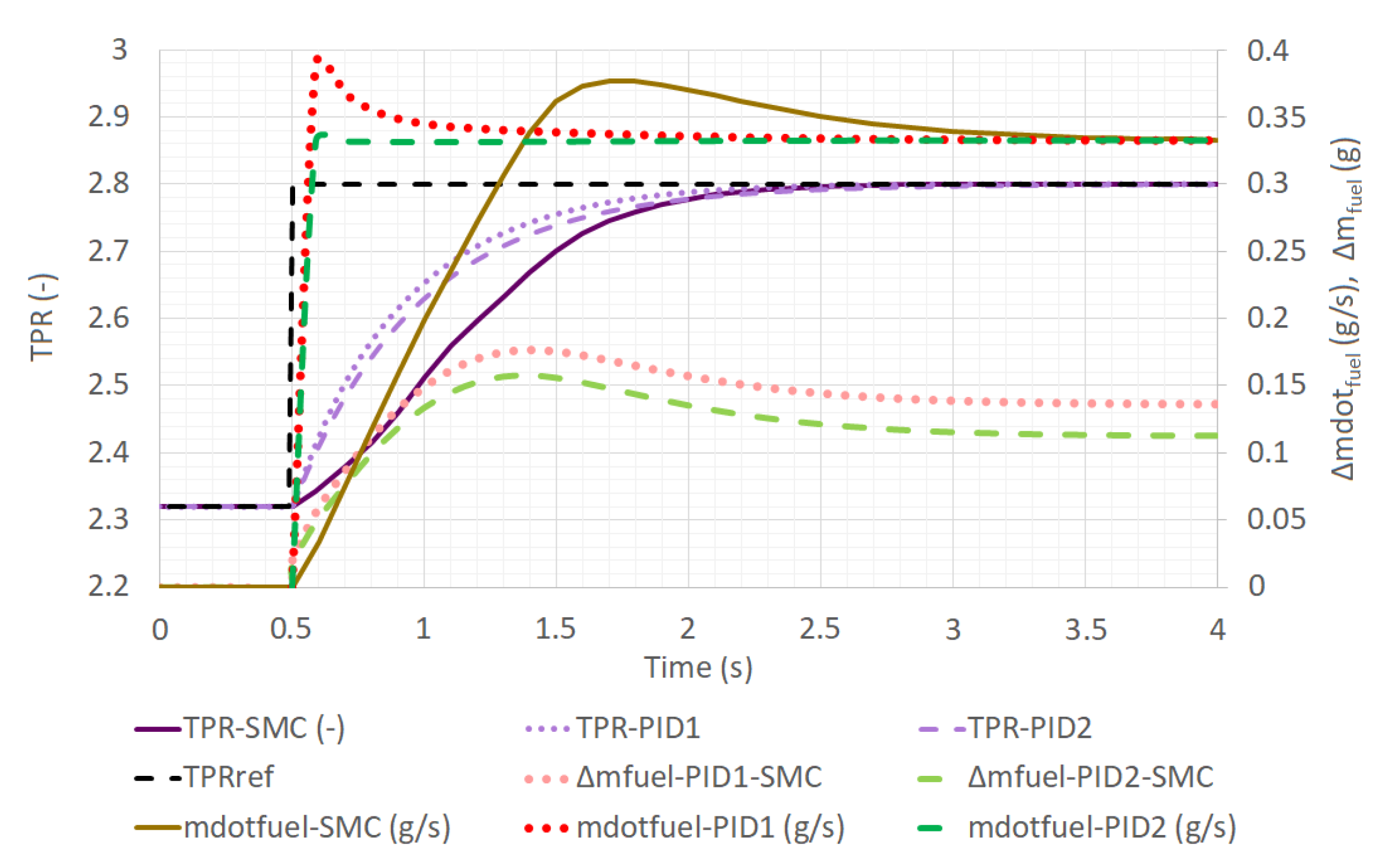
Proportional-Integral-Derivative control systems are very widely spread through the industry, therefore, although they are based on a linearized approach of the plant, a comparison at a specific operating point could reveal the benefits of the sliding mode control. The operating point was selected at approximately cruise power setting, which is the most typical regime of the turbojet. The meaning of the comparison is to show the advantage of the SMC already at a single point.

SMC has a settling time of 1.57 s, and the rise time equals to 1.06 s. There were multiple settings regarding the conventional PID controllers, which attempted to reach similar properties like SMC has. For this reason, the transfer function of the plant has been established at a specified operating point, this was the nominal. The transfer function is shown in (19). The large magnitudes are due to the fuel supply rate being around ${10}^{-3}$ kg/s at TPR with a magnitude of 1.

$$G\left(s\right)=\frac{2.7495\times {10}^9}{s^3+3.612\times {10}^3{s}^2+9.172\times {10}^{5}s+1.905\times {10}^9}$$

(19)

All the PID controllers have been optimized by the integrated tuning tool in MATLAB^® Simulink^®. All controllers have been obtained as a parallel form, shown in (19), with filtered differential output to reduce the effect of input noise. The first PID controller was set to achieve the same settling time with the most possible robustness.

The settings and properties of different PID controllers can be found in

Table 5. Evaluation of different error terms of simulated parameters.

PID Controller	#1	#2
P	$7.717\times {10}^{-4}$	$6.914\times {10}^{-4}$
I	$1.673\times {10}^{-3}$	$1.429\times {10}^{-3}$
D	$1.353\times {10}^{-5}$	$1.007\times {10}^{-5}$
N	4.9892	236.9
Rise time	0.93 s	1.06 s
Settling time	1.57 s	1.91 s
Overshoot	0%	0 %
Gain margin	63.1 dB	64.1 dB
GM angular frequency	955 rad/s	1060 rad/s
Phase margin	$90.0deg$	$90.0deg$
PM angular frequency	2.04 rad/s	2.07 rad/s
Bandwidth	2.35 rad/s	2.073 rad/s

, which shows time and frequency domain values as well. Controller #1 provides equal settling time; controller #2 has equal rise time compared to the SMC system.

There was a selected step response of the system, which can be found in Figure 5, the transient is around 0:01:30 s. The simulation results have been plotted against each other and the fuel mass flow rate has been integrated in order to give consumed fuel mass, where the reference mass was the previous consumption in the steady state before. Instead of showing the real mass, the difference between each PID and SMC is indicated. These time series can be seen in Figure 8.

4. Results

4.1. Assessment of TPR Against Other Control Parameters

As a summary of this assessment, one can state that rotor speed and TPR have enough range to provide smaller magnitude of the signal-to-noise ratio, meanwhile, EPR and TPR have almost linear correlation to thrust resulting in simpler computation in the control system. According to these findings, TPR seems to have benefits over the two other investigated variables, as it offers both advantageous properties; it does give a fair signal-to-noise ratio due to its broad range, and it does not require additional computation to establish linear thrust output, because it changes linearly with thrust.

As a secondary comparison, the SMC control has been adapted to other control laws as rotor speed and EPR. The main structure, which has been shown in Figure 4, has been kept, only the required reference and the sigma calculation have been changed. The corresponding reference signal was taken from the measurement, selecting the appropriate parameter to be tracked by the controller, so the plant was basically regulated like in the main investigation. The main focus during the present assessment was on differences in fuel flow and turbine inlet total temperature, which is usually the mostly limiting factor during the engine operation. The changes due to different control laws in $T_{t4}$ can be evaluated in Figure 9. This diagram shows the values belonging to rotor speed control with a green solid line; the red dashed line represents changes due to EPR control. A third black plot gives an aid to determine what kind of transient is in progress at the given time, basically repeating the TPR reference line from Figure 5. The positive temperature peaks can be dangerous for the integrity of the turbine, therefore, it is necessary to investigate this parameter.

The green curve has more evident changes as the controller results in a quicker response for transients. If the change in demanded value is not too much, the rotor speed controller develops a single peak, which exhibits negative difference during deceleration (see just after 5 s in Figure 9) by reducing the fuel flow more suddenly as it would happen in the reference TPR control. This phenomenon would revert during acceleration; but all other transients including accelerations are significantly larger, and another interesting behavior is then visible, namely, double opposite peaks after each transient initiation. The first peak always points in the direction of the transient, but because it results in a severe over or undershoot of the desired steady-state temperature, a second, opposite direction peak must appear to draw the temperature back to the normal level.

The red dashed curve in Figure 9 shows more disturbed appearance. Basically, the EPR control was found to be perceptibly slower than TPR, this leads generally opposite behavior in contrast to rotor speed regulation, first the fuel injection falls behind the others, resulting in negative temperature difference in the initial moments of an acceleration; then, in order to achieve the desired final value, the temperature must rise beyond the reference.

The next parameter, which significantly depends on turbine inlet temperature and has another important effect on engine stable operation, is the $\varphi$ fuel-air equivalence ratio. In case it passes beyond lean or rich blowout limit, the combustion stops and an accidental engine shutdown occurs. However, it must be noted, that engines are typically more tolerant in case of richer mixtures; before the equivalence ratio could reach the corresponding blowout limit, more violent surge and stall conditions can disturb the stable operation of the engine.

In Figure 9, the reference is given with black dash-dot line, just as in the previous figure, in order to give an aid to identify transient conditions. The basic TPR control equivalence ratio, ${\varphi }_{TPR}$, is indicated with solid a purple line. As it has been previously mentioned, it represents a moderate intermediate solution between faster rotor speed and slower EPR regulators. When comparing green dashed line of ${\varphi }_n$ and the red dotted curve of ${\varphi }_{EPR}$, one can state that there is no extremely large difference, as EPR controller reacts slower, its change in equivalence ratio is very smooth and does not tend to exceed the value of equivalence ratio corresponding TPR control, except for two occurrences. The more problematic tendency is found when evaluating the rotor speed control. This system results in considerably higher peak values in the initial phase of transients, mostly for those transients, which have high, but not extremely large change in the demand. In other words, the third transient, which is the second acceleration in 15 s from the beginning, does not show very large difference between equivalence ratios belonging to rotor speed and TPR. However, those moderate level transitions, like the second transient, or first acceleration, which begins in 10 s, shows a considerably larger peak value of equivalence ratio for rotor speed control. Even if all values fall within the normal stable operating range of the combustion chamber, it must be noted that sudden changes in fuel supply might result in local flameout zones that can induce oscillation and subsequent instabilities first in combustion chamber then in the entire engine.

Just as in the previous figures, green curve in Figure 10 represents rotor speed related values, red line stands for EPR control. The TPR reference shows again for identifying which transient is in progress at a given time. As rotor speed control shows quicker response, it is expected that it will yield an increased amount of fuel consumption. What is rather interesting that the slow EPR control shows in the first half of the simulation shows a considerably higher amount in contrast to TPR as well as rotor speed control laws. The reason is clear, if one evaluates Figure 9, where the corresponding parts have typically higher gas temperatures than the other systems have. Because $T_{t4}$ is an evident indicator of fuel mass flow rate, the latter is not independently included here.

The last comparison is focusing on the amount of fuel consumed during the given transient conditions, as it has shown interesting results. This investigation was based on the integrated fuel mass flow rates of different other control laws and expressed as difference against this reference consumption. The time series are indicated in Figure 11.

4.2. Comparison of SMC with PID Controllers

As a summary of the data obtained from PID controllers, one can tell that they offer more aggressive transient behavior and consequently considerably higher fuel consumption even if they provide similar time domain properties compared to SMC.

According to Figure 8, the rotating speed was rising from approx. 73,000 to 91,000 rpm, i.e., from 60.4% to 75.3% of the maximum, this can be considered as a significant but not excessive acceleration. The final fuel mass flow rate increases from 0.777 g/s to 1.109 g/s, which is 42.7% higher in contrast to the initial value. (As a reference, the maximum recorded fuel consumption was 1.635 g/s during the measurements.)

The difference in consumed fuel amount is also shown in Figure 8, which corresponds to the excess fuel supplied during this transient, in contrast to the amount which is being consumed during the initial steady state operating mode. There are evidently two curves that belong to this concept, with a reference to the SMC, thus the two differently tuned PID systems are compared. Both PID controllers have a final difference slightly over 0.1 g, which is considerably high, if one takes into account, that the initial steady state mode has 0.777 g consumption every second. Throughout the entire four seconds taken into account by this investigation, the total consumed fuel amount can be seen in

Table 6. Fuel consumption of different control methods.

	PID #1	PID #2	SMC
$m_{fuel}$ (g)	$5.498$	$5.475$	$5.362$
$\Delta m_{fuel}\left(\mathrm{g}\right)$	$0.1362$	$0.1127$	0 (ref.)
$\delta m_{fuel}(\%)$	$2.540$	$2.102$	0 (ref.)

. As it can be seen evidently, the difference between SMC and PID corresponds to at least two percent, and in each cases the SMC control offers favorable consumption.

5. Discussion and Proposal of Control System Buildup

5.1. Discussion of Conducted Investigations

Gas turbine engines show strongly nonlinear characteristics, therefore an LPV model has been chosen, which efficiently combines simplicity from a basic linear theoretical background with the adaptivity of the nonlinear models. This LPV model efficiently simulates changing behavior of the engine due to variation of operating modes, and offers the decomposition by TPR itself, i.e., in order to obtain matrix members for a given operating condition, the control parameter is used only. Although the measurement was carried out using a single temperature probe, which can be considered as less reliable due to the non-homogenous thermal field at the turbine outlet, the model performs quite stable, the typical errors lie around 1%, the highest being the error of $T_{t4}$, which has approx. 2% mean absolute percentage error. In order to obtain more accurate values for identification, the measurement system layout should be reworked in order to obtain this critical temperature from more positions that can lead to a better coverage of the real temperature distribution.

The authors have performed two separate measurements, each dedicated to a specific part of the research. As long as the staircase envelope for the control signal with small steps between each stable operating conditions was suitable for the identification of the system, the second engine run with large step transients was more appropriate for inspecting transient behavior of the plant. This solution was selected in order to let the controller face real nonlinear situations and inspect its performance under such circumstances. As the result has shown, the main simulation parameters correctly follow the expectations given by the measurements, slight but not considerable excursion is found only in $T_{t4}$ and at the beginning of transient conditions. The former has been explained above, the latter was also mentioned, namely, the simulation uses a pure step signal to describe the change in reference TPR, in reality the transient was conducted manually by setting the throttle of the remote control to a predetermined value, resulting in a much slower rise of demand, consequently other parameters followed this slow increase. The authors did not consider performing the complete simulation again using more realistic changes in reference TPR, as the obtained results with the present form of the simulation already provide enough accuracy.

Another important consideration regarding the problem of $T_{t4}$ is the usage of state estimator. If the given parameter is not directly measurable or the acquisition of this value results in such inaccuracies which were shown, a typical solution can be the design of an appropriate state estimator, which provides a calculated value for the missing signal. Naturally, the system must be checked for observability, whether the required information can be gained by other measurable parameters. Hence, one must carry out another assessment of observability, which requires a different assumption for output matrix, instead of the one published in (9), namely, the two measurable variables n and $p_{t4}$ are considered as outputs, from which the unknown parameter can be estimated. The corresponding ${\mathbf{C}}_{\mathbf{obs}}$ can be seen in (20) in a transposed form for better layout only.

$${\mathbf{C}}_{\mathbf{obs}}^{\prime }=\left[\begin{array}{ccc}1& 0& 0\\ 0& 1& 0\end{array}\right]$$

(20)

The “sigma for smc” function shown in Figure 4, was expanded and the regarding observability matrix indicated in (21) has been calculated throughout the entire simulation. Equation (21) already takes into account the dimension of the plant, which equals to 3, and similarly to (20), shows the transposed form of the matrix.

$${\mathbf{Ob}}^{\prime }=\left[\begin{array}{ccc}{\mathbf{C}}_{\mathbf{obs}}& {\mathbf{C}}_{\mathbf{obs}}\mathbf{A}& {\mathbf{C}}_{\mathbf{obs}}{\mathbf{A}}^{\mathbf{2}}\end{array}\right]$$

(21)

After running the simulation, it can be stated that the observability matrix holds a constant value of 3 throughout the whole operating range of the engine, i.e., the $T_{t4}$ turbine inlet temperature is observable, if the rotating speed n and turbine inlet total pressure $p_{t4}$ are measured.

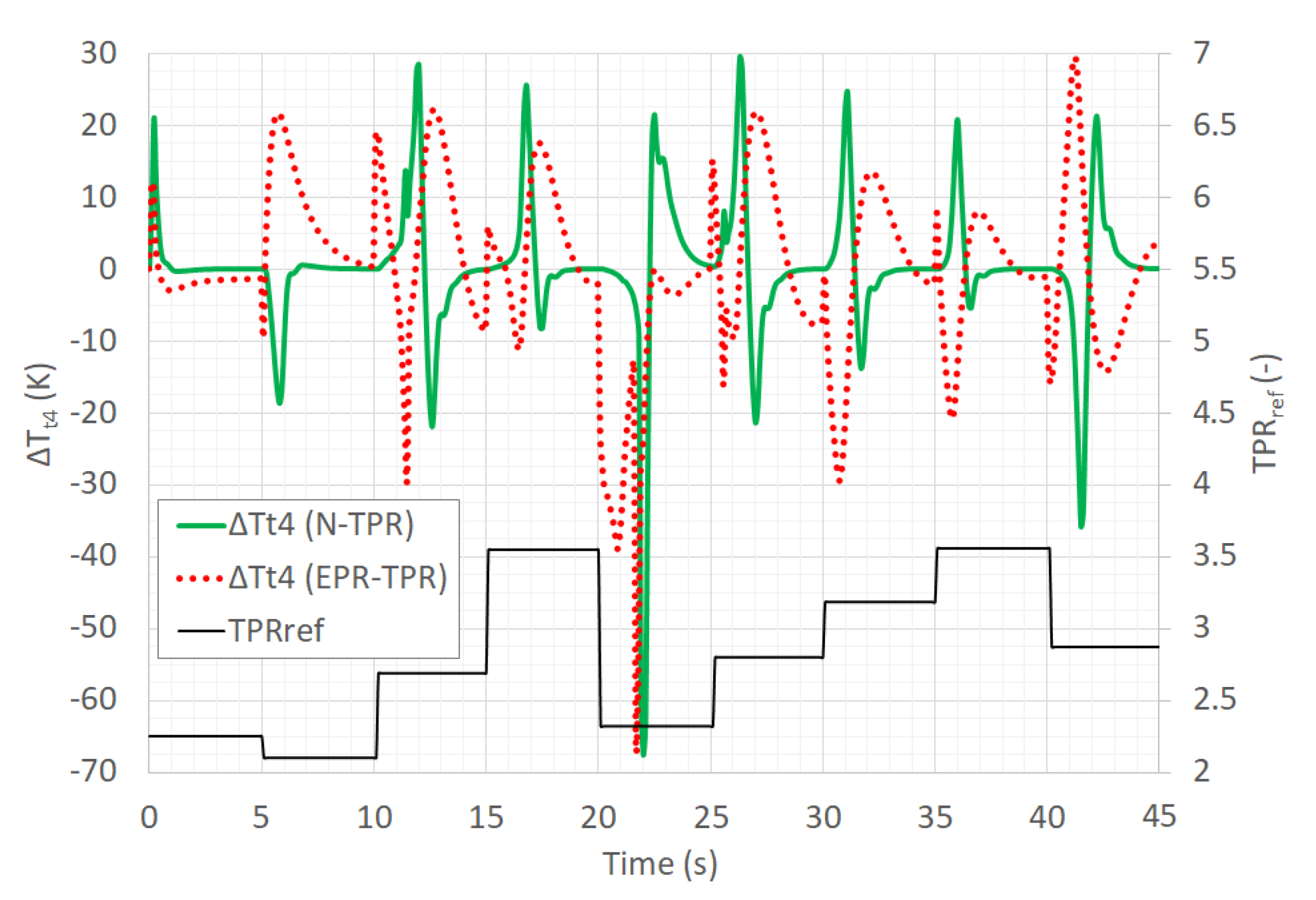
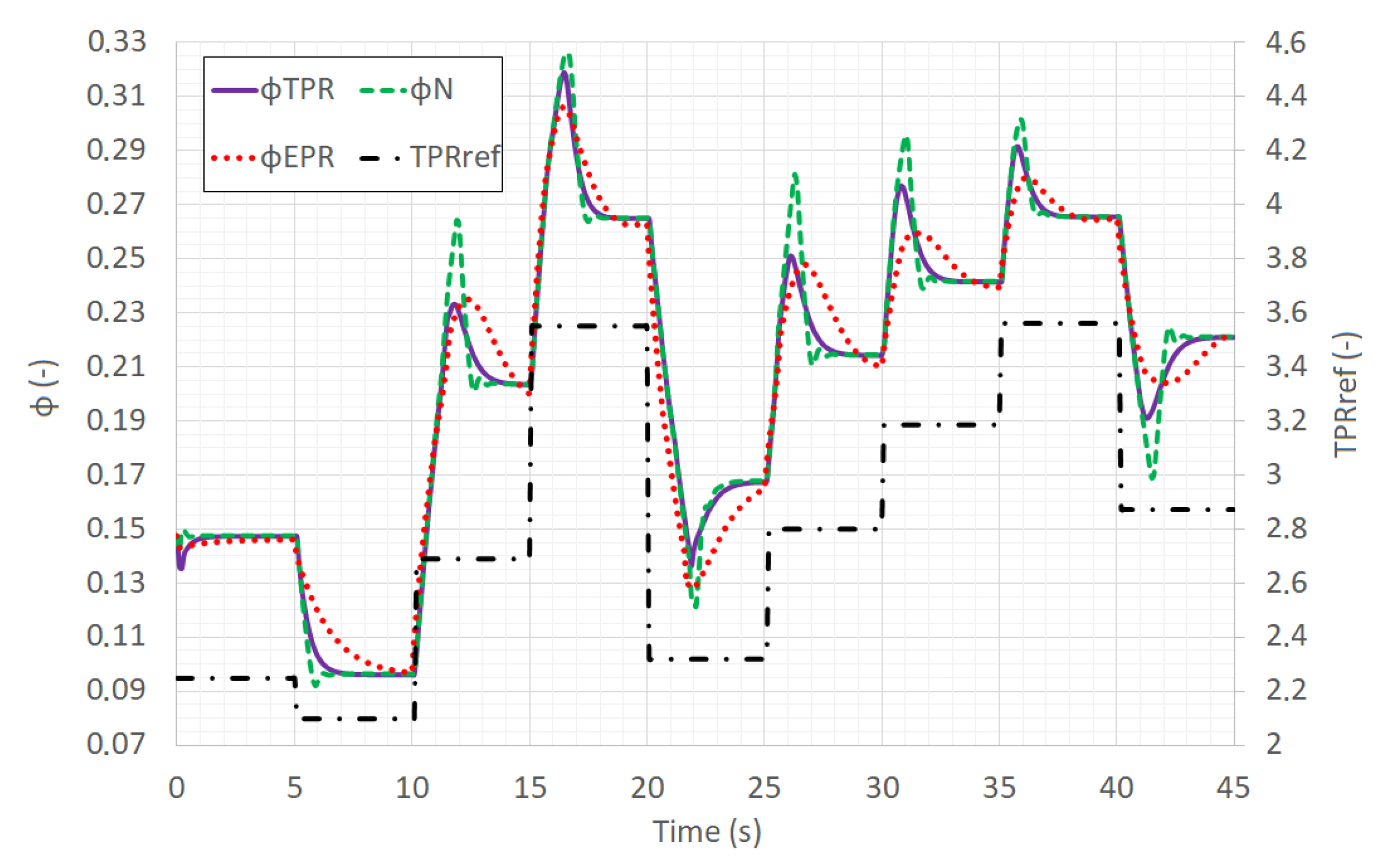
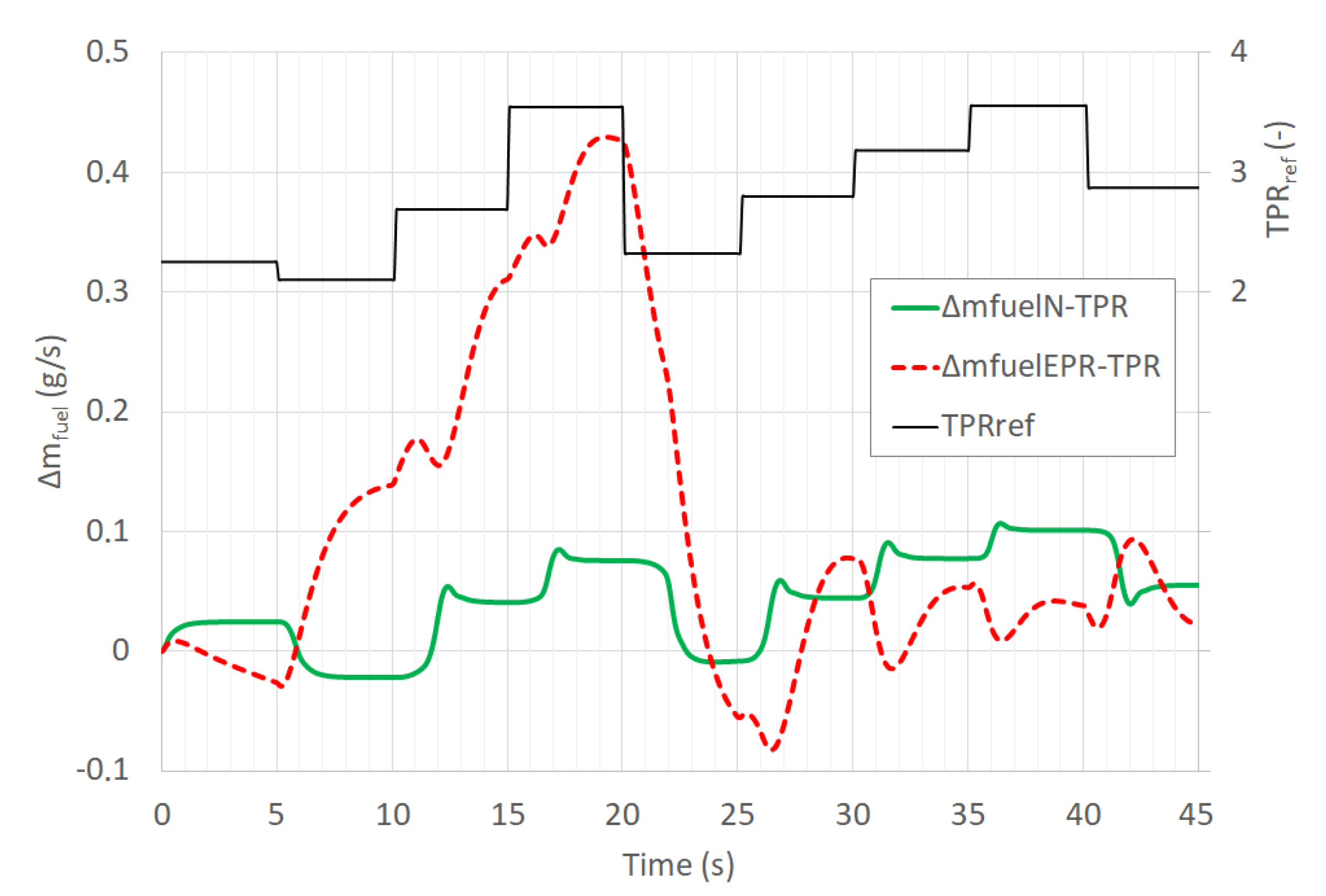
During the comparison between different control laws, the authors have chosen the originally selected time series as reference, adapted to each individual control parameter, i.e., in case of EPR the actual values have been computed throughout the data set and this has been used as demand signal. Even if the reference was in this viewpoint identical for all the three assessments, the different regulation parameters exhibit changes in fuel consumption, peak turbine inlet temperatures, etc.

In the comparison of SMC and PID controls, the emphasis was put on additional fuel consumption due to faster changes in fuel mass flow rate when the system is regulated by PID compensators. When assuming PID, it must be mentioned that the plant is considered to be linear, hence the deceleration will result in the opposite condition, i.e., less consumption is expected for PID. Nevertheless, there are some additional aspects, which have to be taken into account. During acceleration, the excessive increase in fuel supply leads to much higher gas temperatures, probably reaching such values, where limitation must be applied. This condition can completely override the performance of the PID resulting in much slower reaction due to the constraints. On the other hand, when the deceleration is considered, the suddenly decreasing fuel flow increases the risk of flameout and engine shutdown. Another important limit protection subsystem must be implemented in order to prevent the appearance of this extremely dangerous condition.

5.2. Proposal of Control System Buildup

Besides the simulation of the control system, the authors also propose a possible system buildup, based on previous experience with preceding version of PID controllers. As it was discussed in [50], the TPR control has been realized and regulation of the micro turbojet engine has been provided by a simple PID system. The controller was based on an NXP (formerly Freescale) MC9S08DZ60 microcontroller, which provides a maximum of 20 MHz bus clock and an entry-level 8-bit architecture. Despite the legacy hardware configuration, it was able to regulate successfully the PD-60R engine, as it was indicated in Figure 2 and Figure 5 earlier.

In order to establish the possibility for comparison, the proposal is also based on this platform. First, a non-optimized code was generated, which simply copies the commands performed by the MATLAB Simulink function. In this way, the program has to evaluate several expressions which repeat several times, mostly regarding the calculation of the derivatives, see (12)–(16). For preliminary evaluation, when the goal is to determine whether the given algorithm is simply feasible within the required time frame, only the main calculation is tested. There were three additional rearrangements investigated, which result in slightly more optimal solutions.

At the first attempt, the square root function was calculated once, stored in a variable and used subsequently.

At the second attempt, the product of $p_{t2}$ and ${\sigma }_{cc}$ is also stored in a separate variable.

The third optimization technique was to incorporate a square root estimator based on secant method, by transforming the original number into an unsigned integer and increasing the magnitude to ${10}^4$. The principle was used already in the PID control, where no floating point variables were used. The typical temperature ratio does not reach 4:1, therefore the search algorithm is optimized to the maximum of 40,000. In this respect, the maximum awaited square root is 200; the minimum one is 100, assuming the compressor inlet total temperature cannot exceed the turbine inlet value, thus an ultimate minimum temperature ratio is 1:1. As it can be seen, the resulting square root is 100 times greater than the original number, thus, during repeated conversion back to double precision floating point value, the correct magnitude must be ensured by a further division. As this algorithm has a resolution of 0.01, the maximum error introduced by truncated decimals is 0.5%, which can be accepted.

The run time of all cycles have been recorded by using a digital counter and a source of 10 MHz signal. Two other important figures of merit have been checked, the number of variables used and the memory footprint of the given calculation, measured in bytes. Finally, a percentage change in contrast to the previous version is also submitted in the viewpoint of run time. The results are indicated in

Table 7. Comparison of different controller algorithms.

Method	PID		SMC
		orig.	#1	#2	#3
Run time ($\mu s$)	4685.9	22838	9718.2	8250.9	7688.0
Change in run time (%)	-	487.3	42.55	84.90	93.17
Number of variables (-)	30	30	31	32	37
Used RAM (B)	64	240	248	256	266

. It must be mentioned that the original PID method uses unsigned integers as fixed point values, thus the calculation is generally quicker, however, some conversions must be performed, where the inherited 16-bit resolution is not enough; in these cases unsigned long with 32-bit field length is used. The integer variables also contribute to a more compact RAM arrangement. Nevertheless, due to the above mentioned square root estimator, the PID calculation will have an inherent error of approx. 0.5%.

As it can be seen in Table 7, the original SMC implementation would take almost five times more time and memory space. Considering the DZ60 family, which incorporates 4 kB of RAM, the latter is not so burdening, in contrast to the run time, which rises beyond 0.02 s. As the control should be performed real-time, supposing the main routine tested hereby is taking place at an approximate rate of 50 cycles/second, the direct programming of the SMC is not suitable. If one changes the code and calculates square root at the beginning of the cycle, then this result is substituted into subsequent steps, one can gain significant time. The #1 solution has a considerably shorter period of slightly less than 0.01 s. Taking into account other tasks to be executed (like the event driven analog-to-digital conversion, etc.), one can state that this solution is already feasible. Nevertheless, in order to increase the overhead in the viewpoint of run time the second solution with a priori multiplication can cut further 15%, finally, when using unsigned integer square root estimation, despite the 0.5% error, the run time can be decreased by an additional nearly 7%. Among the SMC routines, the last one bears 33.66% total time in contrast to the initial routine. Therefore, the last one surely can serve as a basis for realization of the control system. Furthermore, it can be noted, if up-to-date microcontrollers are chosen, the 32-bit architecture and significantly increased clock rates of at least 50 to 100 MHz will result in considerably better performance.

6. Conclusions and Future Work

This article showed the design and evaluation of a SMC based on TPR for a micro turbojet engine. The authors have briefly described the LPV model of the engine, which was identified using real-world measurements of a selected type, PD-60R. The SMC is based on error and error derivative, therefore, due to the unconventional thrust parameter, the derivatives were also deduced during this investigation. The primary examination of the mathematical was performed using a measurement in which the engine was operated at different stable TPR levels for prolonged periods and sudden transients were made in both acceleration and deceleration. The results show only a small percentage of errors, i.e., the model is able to describe the plant behavior according to the expectations. Using the same time series, the controller could also be inspected and was able to regulate TPR to the desired value within a mean absolute percentage error of 0.6%. Thus, the conclusion can be drawn, SMC is suitable even if TPR is used as thrust parameter.

Furthermore, the authors conducted a thorough assessment of the controller including comparison with other control laws like rotor speed and EPR, and another part, which focused on different control methods of PID. In both cases, the lead of TPR and SMC was shown evidently through various simulations. The TPR/SMC control combination proved to be superior to all other solutions in regards of temperature profile, equivalence ratio, and total fuel consumed during the given transient.

The authors have investigated the possibility of creating a real control system, and it was also proven that the SMC program can run even if an entry-level, 8-bit architecture microcontroller unit is used. It has been also taken into consideration that according to the experience of performed measurements, the acquired turbine inlet temperature signal exhibits significant anomalies in contrast to predicted model values, which is considered to be the result of a single thermocouple immersed into a largely non-uniform temperature field. In order to overcome this, the possibility of a minimum-order state observer has been investigated and it was found that the LPV model provides observability throughout the entire operating range of the engine.

When considering additional computational tasks like state observer, the original assumption of 8-bit microcontroller must be abandoned. In such a case a more agile unit should be chosen, the same semiconductor manufacturer offers e.g., LPC1768 series, which is a 32-bit Arm Cortex-M3 processor running at a maximum of 100 MHz clock frequency, which is at least 5 times quicker than the legacy hardware. Besides the significantly improved speed, it also incorporates more memory, with 512 kB for a more complex firmware and 64 kB static RAM for data handling. The unit also allows higher levels of communication like USB and CAN. Its analog connections include a single channel 10-bit Digital-to-Analog Converter beyond the conventional 8-channel 12-bit Analog-to-Digital conversion. The former can be used to directly command the part which is responsible for fuel metering (in the particular case, the speed of the electric motor that drives the fuel pump). If the SMC would be implemented in such a modern microcontroller, it would have enough computational overhead for future expansion of the system, even if the state observer is included together. Such further improvements could involve automatic starting, protection against hazardous operational circumstances like overspeed, condition monitoring and diagnostic system for the engine, based on thermodynamic and vibration signals as well.

Additional future work must focus on the behavior of TPR throughout the entire flight envelope, which will require a comprehensive analysis assisted by experiments with either flying test bed or an altitude test stand.