Abstract
The paper discusses the possibilities of objective assessment of military flight training quality based on statistical evaluation of pilot’s behavior models parameters. For these purposes, the pilots’ responses to non-standard flight situations were measured by using a fixed-base and a moving-base engineering flight simulator. Tens of military pilots at different training stages were tested. By exploiting real-life tests, we established that the given pilot models provide sufficiently accurate approximation of realistic human responses. Importantly, the models are relatively easy to use, and the individual parameters can be unambiguously interpreted, i.e., the time constants of the pilot behavior model are obtainable, representing the pilot’s current psychological and physiological state of mind. The parameters lay in the defined ranges, and they characterize the ability of the human/pilot to adapt to a controlled dynamic system. Consequently, a fundamental statistical analysis based on pilot’s behavioral model parameters was conducted, using the acquired test data representing the pilot’s behavior during repeated measuring. The initial results indicate the possibility to use the results for objective assessment the military flight training level.
1. Introduction
Contemporary aviation places increasingly more emphasis on the mental stability of both the pilots and the supporting personnel. In addition to the traditional factors that complicate their work performance, including noise, vibration, overload, and changing air pressure, these professionals are required to operate new technologies whose complexity and control configuration features (despite the high degree of automation) often put whole crews under significant stress [1]. The problem is exacerbated by the fact that most of the skills utilized by pilots for fast and reliable operation of the systems deteriorate during flight downtimes. Piloting, in its pure form, together with the development of technologies, has receded into the background to be replaced by the need to operate navigation systems and autopilots. Airplanes are presently capable of performing autonomous take-off and landing; the pilot, however, still plays a crucial, irreplaceable role in the decision-making process [2].
Aviation generally needs to recruit specialists with qualities that contribute to flight safety; these comprise, above all, spatial orientation, movement coordination, motivation, resistance to stress, cooperative mind, responsibility, and the ability to lead. However, there is no uniform pattern of what qualities should a pilot have. The requirements placed on groups of pilots then form another specific domain, where communication, coordination, and resistance to monotony and stress are the know-how to be adopted by each transport pilot. In contrast, fighter pilots need to exhibit high perceptual speed, responsiveness, and resistance to g-force and time stress. By further extension, helicopter pilots should excel in coordinating their hand and leg movements and concentration capabilities.
In aviation, the human factor plays an important role, and a potential human failure could lead to poor flight performance, an accident, or even a disaster. The study of the relationships between diverse human factors and flight performance or activities related to flight safety thus embodies an important research domain where aircraft design, pilot selection, and operation environment constitute major sub-problems. The effect of such an investigation is defined by links within the SHELL (Software, Hardware, Environment, Liveware/human being to Liveware) conceptual model [3], in which the most important link is human–human. Historically, it was human skills that facilitated the birth and progressive development of aviation technologies; gradually, however, people have become the weakest element in the entire system. This is also why only selecting the best individuals does not suffice for the reliable performance of the pilot profession. Significant aspects consist in effective management and use of the training time, with adequate practice needed to refine the potential of future pilots. Thus, aviation personnel training is a lengthy and demanding process that often involves the most advanced knowledge from psychology, physiology, and IT.
Pilot behavior modeling remains an open topic, wherein the tasks are usually solved by structuring the active (for example, voluntary, behavioral, and low-frequency) and passive (involuntary, biodynamic, and mid-frequency) activities, according to the fixed wing aircraft classification. Based on this approach, the active pilot activities relate to phenomena, and the pilot response is connected with flight dynamics, whereas the corresponding passive activities are related to aero-elastic responses.
The initial hypothesis for our experiments is that the pilot’s ability to control the aircraft reliably and safely increases with the training. Therefore, there is a certain opportunity to try to measure, test, or evaluate the state of pilot’s ability to control the aircraft appropriately and objectively. The goal of our research focuses especially on experiments to support pilot behavior modeling analysis in association with military flight training, using flight simulators. The nature of this approach lies in repeating measuring the pilots’ responses to a visual stimulus and consequent identification and evaluation of the pilot’s behavioral model parameters, such as reaction delay or lead/lag constants as the so-called equalization part responsible for pilot’s ability to adjust to the controlled dynamics and his/her attitude to control. The resulting parameters can then be used for the following:
- -
- Finding common features in the pilots’ behavior during flight control,
- -
- Finding the behavioral changes during military flight training and under different influencing factors,
- -
- Comparing the control quality of young, less trained pilots with pilots who have completed 400, 500, or more flying hours on real airplanes, not just simulators.
In terms of the contents, Section 2 provides the mathematical background to pilot modeling techniques; Section 3 describes the experiments and example of identification of the presented model parameters; and Section 4 delivers the experimental results with statistical analysis and assessment of the pilot training based on an evaluation of the behavioral model parameters. Section 5 then provides relevant conclusions.
2. Mathematical Background to Pilot Modeling
The ability of a human being to fly an airplane implies processing diverse information, including the transfer of such information to corresponding movements of the airplane control units. Thus, during this process, the pilot performs the function of an adaptive biological controller. Real-life human behavior, especially when “control tasks” are being executed, is hardly stationary in time, mainly due to fatigue or loss of attention. In addition, there are several such tasks where the operators must adjust their strategy due to changes of the vehicle (aircraft) dynamics in time [4,5].
Based on the information presented in the relevant studies [1,6], the human behavior during a control task can be described by using Rasmussen’s general model. It consists of several levels for different types of control. These levels are as follows [7]:
- -
- Control level (compensatory feedback control),
- -
- Coordination level (control based on rules),
- -
- Organization or cognitive level (control based on knowledge).
When modeling pilot maneuvers, it is important to identify the central factors of the simplest possible model that still maintains the main behavior and complexity of the pilot modeling [8]. Most of the approaches are focused on the modeling of the lowest level of human behavior model (control level), because it is responsible for fast reaction to changes and contingencies, and it is one of the most important parts influencing human control and his/her dynamic properties.
Compensatory feedback control was carefully researched for controlling activities, where the human factor could perceive only one controlled variable and other influencing parameters were unpredictable. Much of our current knowledge originates from research of human dynamics during compensation control tasks with one feedback loop [6,9]; this investigation also showed the complexity of studying the human control process and the ability to adapt to various tasks, namely environmental, control, and procedural variables, as they are summarized in the comprehensive overview proposed in Reference [9].
For the purposes of the research presented herein, we used the simplest system with manual operation, namely a single loop compensatory setup with visual stimulus (Figure 1).
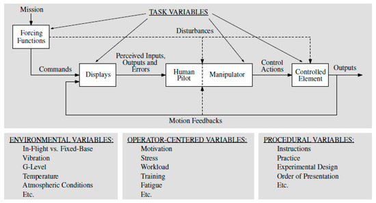
Figure 1.
Single-loop compensatory tracking tasks (based on Reference [1]).
During the compensation phase (using compensatory feedback control), the human regulator works only with control error between the system output (e.g., the flight altitude) and so-called “forcing function”. This function is a random function having stationary or quasi-stationary features (e.g., requirement for the step change of flight altitude) and represents an input signal. Usually, the pilot is expected to minimize the deviation, meaning that he or she is trying to maintain the flight parameters at the required levels defined in the task. The error is minimized via the pilot’s control activity. The error signal, showing the difference between the “target forcing function” and the output (response of an aircraft dynamics), is shown on the display, or the altitude meter in this case. During the control activity, the pilot operates the aircraft dynamics visually, while actively controlling the aircraft movement, in order to minimize the difference between the input and the output signals. This task allows frequency response identification, which defines the pilot behavior and control activity.
Mathematical models of human behavior as a controller at the control level have been described in several dedicated studies [10,11,12,13,14]. Among the outstanding specialists in this area is Prof. D.T. McRuer, whose “Crossover Law” [6] became the starting point for many follow-up experiments and papers. McRuer’s theory showed that, after accepting certain simplifications, human behavior (his/her dynamic properties) can be described by using the theory of dynamic systems and theory of automatic control. Based on this theory, researchers characterized and verified many types of human behavioral patterns for simple controlled dynamics [15,16].
By generalizing the theory of Crossover Law and the associated models, human (a pilot’s) behavior can be simplistically described via a transfer function, as shown in Equation (1). The equation describes the dynamic model of human behavior at the control level as a ratio of Laplace transform of an output signal (pilot’s control action)—Y(s) and human pilot’s input signal (perceived input)—U(s) and is valid for the SISO (single-input single-output) generic controlling dynamic systems.
The first of the model parameters, K, is referred to as the amplification or gain, which represents the pilot’s habits for the given control action and relates, to some extent, also to the ratio of the output and input signal. Another part of the equation, the “equalization part,” defines the way the pilot adapts to the controlled system and its dynamics. The basis for the pilot’s adaptation consists in the ratio and form of the numerator and the denominator polynomials provided by the values m, n, and q, defining the general structure of the human-pilot behavior model. There are several rules leading to choice of these parameters defining the model structure. Considering the causality of the model, the numerator order must be higher or equal to the denominator order (relation between q and m, n values). The dynamic properties of a controlled element also influence the choice of these parameters, as the Crossover Law defines [6]. Moreover, increasing values of m, n, and q parameters bring more precise approximation of human behavior. According to the abovementioned information, the choice of model structure is especially based on the character of the pilot’s response during control of a certain dynamic system, e.g., an oscillating pilot response requires inclusion of oscillating component (n > 0) into the model, or, vice versa, the absence of oscillations defines the model structure as an inertial system (m > 0, n = 0). Exploiting the multiple experiments characterized in References [6,17] and other sources, we established that, to approximate the control actions (namely, to describe human behavior), the structure is usually sufficient where the values of the m, n, and q parameters range most often as follows: q = 0–1, m = 0–2, and n = 0–1. There are, of course, even more complex models, which imply higher orders of numerator and denominator polynomials (see, e.g., Reference [10]). These models, however, are used in particular to refine the model at high values of the frequency characteristics or in rough approximation of some nonlinearities.
Apart from the structure of the model itself, the individual parameters TL, TI, ω, and ξ are also very important. These parameters—the parameter ratio, in particular—define, specifically, the resulting control action. For example, the ratio of the time constants TL and TI describes, primarily, the method and approach to control. For the derivative, the lead time constant, TL, reflects the pilot’s ability to predict the given situation, whereas the TI constant, conversely, reflects a certain inertia or lag. The values of the frequency (ω) and damping (ξ) indicate the presence of an oscillating component.
The last part of the equation embodies the reaction delay, τ, which is related to the registration and subsequent processing of the visual information. The range where the value of this parameter is usually found was experimentally set to (0.2–1.5 s) [11,17]. The reaction delay is a rather critical parameter, as a situation with an excessively high reaction delay could result in a failure of the pilot’s control abilities and the subsequent destabilization of the controlled system. Such a precondition could lead to catastrophic consequences, or, more narrowly, pilot-induced oscillation. A non-negligible fact contributing to the problem lies in that an increase of this parameter can be caused by, for example, fatigue [18].
3. Assessing Pilots’ Training Phase and Experience
Various researchers are using aviation simulation technologies, in relation to pilot modeling, to increase aviation safety [19,20]. One of the methods to assess objectively a pilot’s current state or training level is based on monitoring alterations of his or her dynamic behavior in time, i.e., at different training stages. The change of dynamic behavior is represented by values of individual behavioral model parameters such as K, TI, TL, ω, ξ, or τ. This assessment involves the measurement and analysis of the pilot’s responses by using a flight simulator.
To acquire pilot responses to mainly visual stimuli, two available simulators were used—a fixed-base engineering flight simulator equipped with X-PLANE 10 Pro software (see Figure 2a) and a moving-base engineering flight simulator based on Flight Gear software solution (see Figure 2b).
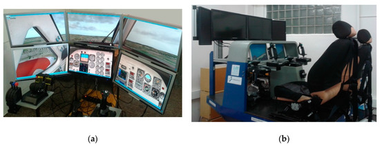
Figure 2.
The flight simulators in use—(a) the fixed-base flight simulator and (b) the moving-base flight simulator.
Both simulators use software that enables the data recording of flight parameters during simulated flight, such as stick deflection, engine thrusts, flight velocity, flight altitude, angle of attack, etc., with sampling frequency up to 20 Hz. The data acquired from these mathematical–physical calculations in real time are extremely precise, with minimum deviation from the real preset situation.
The basic principle of the applied approach (in case of both flight simulators in use) rests in repeated measurement of the response, namely, the pilot’s reaction to a visual stimulus. In our research, the visual stimulus was a simulated step change of the flight altitude, H, indicated by an altimeter. The pilot’s task consisted in reaching the original flight level (flight altitude) as quickly as possible, using solely the joystick deflection (dv).
The selected aircraft was King Air C90B and the initial flight mode was defined as altitude 2900 ft and speed 170 mph, and the angle of attack and pitch angle, including their change, was approximately 0 (note 1 ft. = 0.305 m and 1 mph = 0.447 m·s−1). At a certain time, the altitude was step-changed to 2600 ft., and the task of the pilot was to correct the altitude back to the original 2900 ft., where the current altitude was indicated by the altimeter.
The repeated measurements with the same pilots under the same or similar conditions, using the aforementioned flight simulators, were performed. Data representing mainly altitude, H (perceived input signal), and stick (joystick) deflection, dv (pilot’s control action), were acquired as a result of the measurement for the following data processing and parameters identification of the pilot’s behavioral model. An example of the measured data is in Figure 3.
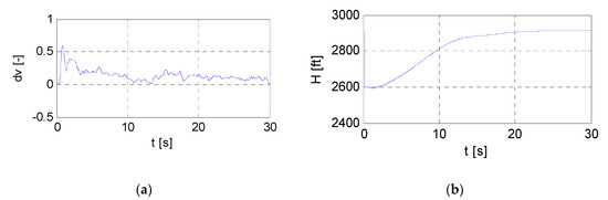
Figure 3.
Data representing pilot’s control action (stick deflection) (a) and as a response to the initial step change of altitude (perceived input signal) (b).
The measured data and character of the pilot’s response enabled us to select the structure of the pilot’s behavior model (see the description in Section 2) and to identify the model parameters.
The model structure had to be chosen with respect to the character of the measured pilot’s response, i.e., the dynamic behavior of the controlled system. One of the most extensively used models is the transfer function in the form of Equation (1), with parameters q = 1, m = 2, and n = 0. The resulting form is then described by Equation (2):
The illustrated model constitutes a general model with parameters K, TL, TI, and τ, described in the previous chapter, and can be utilized in a wide range of controlling or piloting activities; its properties and application possibilities are discussed and analyzed in References [17,21].
Based on real-life measurements, it was further determined that this model provides a sufficiently accurate approximation of most real human responses, [17,21]. The indisputable advantages of this model are its ease of use and the option to define a physiological interpretation of the individual parameters. The time constant, TN, is a parameter describing the dynamic properties of a human-pilot neuromuscular system, and its value tends to be relatively small (0.05–0.2 s). The TL parameter relates to the prediction ability, while TI expresses a certain inertia or lag and dampening of rapid control actions. The ratio of these constants describes the character of the control action—slow and damped if TI > TL, or vice versa, and fast with derivative features if TI < TL. The values of these parameters are most often in the order of seconds. The remaining parameters, i.e., the gain, K, and the reaction delay, τ, were, together with their properties, discussed in the previous section.
Utilizing the experience from the experimental measurements and evaluations of the pilots’ responses, we also used other model structures, especially when oscillations in the response were observed. For these purposes, the model in the form of Equation (1), with q = 1, m = 0, and n = 1, proved to be appropriate. The resulting model is then represented by Equation (3).
The meaning of the parameters gain (K), derivative/lead constant (TL), and reaction delay (τ) of Model (3) is similar to the previous model, Model (2). Frequency (ω) and damping (ξ) characterize the oscillating component of pilot’s control action.
Model (3) is expected to find application in cases of more complex dynamics of the controlled element, such as dynamic, non-minimal phase systems. As an example of a system with non-minimal phase, a dynamic model of flight can be presented.
By identifying the parameters of the presented models, it is possible to evaluate the actual state of the pilot in terms of his/her dynamic properties; if these parameters are then monitored in time or at different stages of training, we can use this information to assess the achieved training level [17].
Various types of tools implemented in MATLAB were employed to identify the parameters of Models (2) and (3). One of the options was the identification algorithm based on the fminsearch simplex function, using the criteria function calculated as a sum of deviations squared; another one consisted in System Identification Toolbox. The properties of these approaches were compared in Reference [21].
A detailed description of the experiment can be found in Reference [17].
4. Evaluation and Results
The authors’ research focuses on assessment of the human factor in aviation, with relevant aspects of interest being pilots’ flight control abilities, military flight training quality, and long-term data acquisition and analysis to facilitate statistical description of the parameter ranges of the behavioral models. The aforementioned parameters of the behavioral models, such as K, TI, TL, ω, ξ, or τ, describe the dynamic properties of pilot’s behavior and provide information about a pilot’s attitude to control. The applied approach is based on measuring the pilots’ responses to a step change of an altitude using flight simulator(s), as described in the previous section.
4.1. Statistical Evaluation of the Selected Parameters of the Behavioral Model
Based on the described principle, a group of 10 military pilots at different training stages was tested on the moving-base flight simulator (see Figure 2b) equipped by Flight Gear software. Each of the individuals underwent 10 repeating tests. An example of the measured data for Pilot No. 1 is in Figure 4.
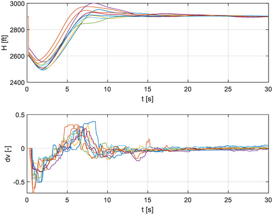
Figure 4.
Data representing altitude, H—perceived input signal (upper) and control action (bottom) of Pilot No. 1 (10 repeated measurements).
The controlled element dynamics exhibit a relatively strong non-minimum phase; this property is observable in the graphs representing altitude H (see Figure 4) in the form of “undershoot” as a response to sudden change of the pilot’s control actions. The related pilots’ control actions correspond to this effect, i.e., the presence of oscillations is observed in most cases. This fact led to the actual use of Model (3). The applied identification tool was based on our own approach, utilizing the fminsearch simplex algorithm [21].
Assuming that the histogram graphically represents the distribution of the selected data in the form of a bar graph, with all columns exhibiting the same width, we can employ it to express the variance of the observed model parameters of the pilots’ analyzed behavior during the compensatory feedback control phase represented by pilots’ response to the step change of flight altitude, H. Various mathematical expressions were defined for several interval widths (classes), and all of these had been derived from the statistical processing of the input data [22,23]. In the actual pilot testing, we applied the number of analyzes carried out in each flight task with identical flight parameters and the same analyzed parameters (the necessary precondition is the same simulator). From the performed mathematical analyses and information reported in the literature, it can be assumed that the histogram data files have a normal or another standard distribution with a probability of appearance of some outliers. The results yielded statistical information about the possibilities and limitations of the pilots, in general [24,25].
Figure 5 and Figure 6 present an evaluation of the individual parameters of the pilot’s behavior Model (3) for the aforementioned group of military pilots. All of these histograms exploit the statistical dataset, including approximately 100 values (10 test measurements per 10 pilots). The outliers are neglected. The distribution of the individual parameters is, in most cases, similar to the log-normal distribution, corresponding to the expectations, as the log-normal distribution of probability is often connected with the human factor.
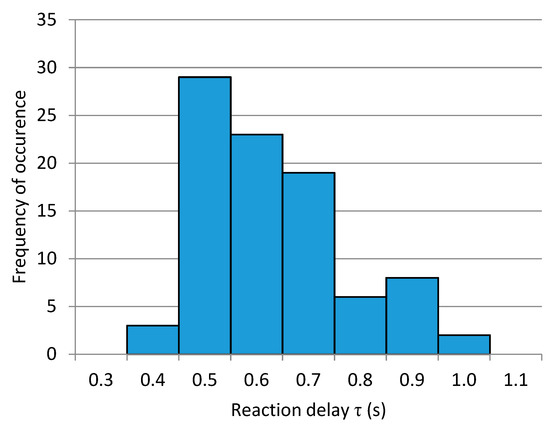
Figure 5.
Histogram depicting the distribution of reaction delay parameter for the group of 10 military pilots.
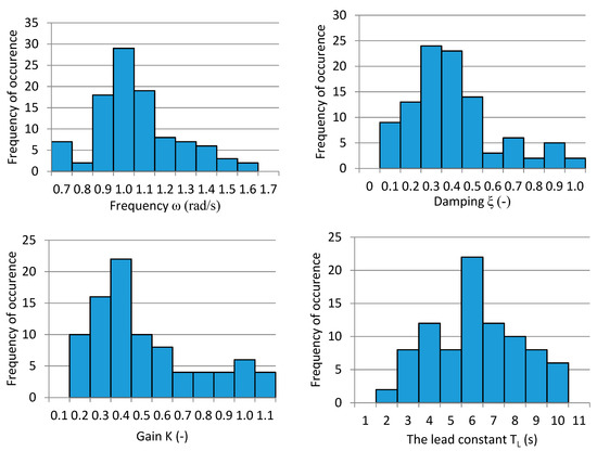
Figure 6.
Histograms depicting the distribution of parameters of Model (3) for the group of 10 military pilots.
The first and, at the same time, one of the most important parameters is the reaction delay, τ. The evaluation of this parameter is included in the histogram in Figure 5. The most frequently occurring value of this parameter reaches about 0.5 s, a level typical of such human (pilot) activities [26].
As mentioned in the preceding section, the reaction delay, τ, is one of the most important parameters. The quantity relates to the visual information processing time, and its value has an invariably negative influence on the controlled process, or flight control in the given case.
Other significant information about the human/pilot behavior or dynamic properties related to the described task is outlined in Figure 6. The frequency, ω, with a most frequently occurred value of about 1 rad/s, describes—together with damping, ξ—an oscillating part of the pilot’s responses. The most frequently occurring value of damping, ξ (about 0.3), indicates the presence of oscillations that are only slightly damped. The gain, K, and the lead time constant, TL (with the most probable, and relatively high, value of about 6 s), define the character of the pilots’ control action as a derivative—fast and more aggressive.
4.2. Assessing the Pilot Training Based on the Evaluation of Behavioral Model Parameters
As an example, two independent sets of test results are presented, both performed with seven military pilots completing 10 flight tasks. The participants were students (pilots) in the fourth year of the bachelor’s cycle of study at the Air Force and Aircraft Technology Departments (Faculty of Military Technology, UOD), meaning that they shared the same or similar levels of training. Both sets of tests were carried out under identical conditions on the fixed-base engineering flight simulator (see Figure 2a) equipped with the professional X-PLANE 10 simulation software [21]; the unit is operated by the University of Defense in Brno. The time interval between the first and the second measurement sets was approximately six months. During this period, the pilots also underwent the required military flight training, which included, inter alia, the flight practice of approximately 20 flying hours. Due to those, pilots were only in initial flight training, meaning that they had about 100 flying hours, in total, and those 20 h are approximately 1/5 of their overall practice, i.e., the impact of the training will be greater than for an experienced pilot with hundreds or thousands of flying hours.
For this study, the Model Equation (2) was employed in the modeling of the pilots’ behavior. Based on the previous experience, the model provided sufficient approximation of the pilots’ responses during testing on this type of simulator. The applied identification tool again exploited our own approach, using the fminsearch simplex algorithm.
The identified parameters K, TL, TI, TN, and τ (see (2)) for each pilot and flight task can be viewed as statistical datasets, and their basic characteristics can be specified. As mentioned above, seven pilots participated in each measurement set, with each of the participants subjected to 10 repetitive flight tasks; in total, 70 cycles were thus carried out for each set. Although the entire group is not large in terms of statistical significance, the results show that the repeatability of the measurements with respect to the variance of the parameters is satisfactory.
Apart from the histograms, the method to evaluate such a statistical dataset consists in drawing box graphs; these are appropriate for the evaluation and comparison of two or more statistical sets. The box graphs for the individual parameters and measurement sets are depicted in Figure 7, Figure 8 and Figure 9 and demonstrate the distribution of the individual parameters for each measurement set. The area marked with the black line represents the range of the given parameter at the significance level of 5%. The blue-bounded section (box) denotes the area defined by the lower and upper quartiles, i.e., it contains the upper 50% of the dataset values; the red stripe then marks the median. The red crosses represent the outliers.
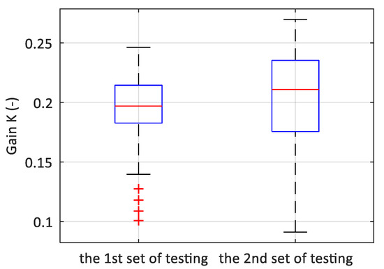
Figure 7.
The box graphs for the parameter gain, K.
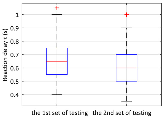
Figure 8.
The box graphs for τ parameter.
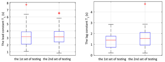
Figure 9.
The box graphs for lead TL and lag TI time constants.
The first parameter to be evaluated is the gain, K. This parameter describes the habits practiced by the pilots when executing a control intervention (action), and, together with the control constants, TL and TI, it defines the resulting response dynamics. The graph—Figure 7 clearly indicates that, in the second set of measurements, the interval of values in which this parameter may be present was extended. At the same time, however, the median was shifted upward, to increase the gain value from 0.19 to 0.21. This fact reflects a rise in the control process speed, meaning that the pilots generally achieved the desired value more quickly.
The second parameter subjected to evaluation is the reaction delay, τ, in which a marked decrease can be observed, see Figure 8. The median value moved up to 0.05 s between the first and the second measurement sets; such a change is satisfactory, considering that the character of this parameter as the reaction delay relates to the registration time and the subsequent processing of the visual information. Reducing this time has a positive impact on the eventual regulatory process.
The box graphs provide a statistical evaluation of the individual parameters; the results, however, can be evaluated also in relation to the individual pilots. We therefore computed the average values of the reaction delay, τ, for the individual participants and each testing set. The relevant values are summarized in Table 1.

Table 1.
Mean values of pilots’ reaction delay τ (A—the first testing set; B—the second testing set).
The other pair of parameters comprises the control constants TI and TL, whose ratio is related to the way the pilot adapts to the controlled dynamics and determines (together with the gain K) the basic dynamic properties of the human controller. At the same time, these parameters account for the prediction ability (TL) and a certain inertia or lag (TI).
In Figure 9, a difference is seen, especially in regard to the TI values. In terms of the controlled dynamics, this effect relates to a certain degree of suppression (or damping) of fast and sudden control interventions, causing reduced oscillation in the resulting transient process.
The last parameter of the model rests in the neuromuscular time constant, TN. The parameter characterizes the dynamics of the human neuromuscular system, which, in the case of Model (2), is approximated by the inertia formula (TN s + 1). It is a parameter whose values range from tenths to hundredths of a second, and its value should be—together with the time, namely the training stage—virtually invariable. This effect was also confirmed in the individual tests, as shown in Table 2.
Table 2.
Mean values of pilots’ neuromuscular time constant TN (A—the first testing set; B—the second testing set).
5. Conclusions
Based on the acquired test data and the created pilot’s behavior models, we performed a statistical analysis accentuating comparison of the transfer function time constants for the pilot behavior model to the training phase and training level of the individual pilot groups. These groups differed in the amount of flight hours spent in real aircraft and also in the actual level of theoretical knowledge. A connection was found between the pilot training stage and the time constants, assessing the pilot training phase and experience.
The graphs and tables show that the pilot behavior model parameters were statistically evaluated and the influence of the individual parameters on the simulated flight control process discussed. The resulting parameters and their ranges correspond to the experimental values referred to in the relevant literature mentioned above. Changes of the parameters in time, depending on the training level, indicate the possibility to provide up-to-date information about the impact of training on the pilots. Conversely, statistical evaluation of the pilot’s parameters at different training stages provides useful data about the possibilities or abilities and limitations of the human controller for the defined task. Such knowledge is also important for the purpose of general human behavior modeling.
One future goal of the authors is to implement the methods and outcomes into effective ground pilot training within both civilian and military aviation training. The whole flight simulator engineering setup could serve as the test station to assess the pilot’s current condition. To pass a task, the pilot needs to be concentrated, well-rested, and have sufficient training. These preconditions bring training flight conditions as close as possible to the real-life flight mode. From the transfer function parameters, the instructor should be able to determine whether the pilot is airworthy or needs to be trained further. Human behavior prediction in aircraft control and the corresponding pilot modeling can contribute to the prevention or reduction of negative effects generated by the human factor in aviation.
Although we were not able to find comparable assessment of the level of training according to the NATO STANAGs regulations (or EASA for the civilian aviation), we are expecting to open this topic in the future, at NATO negotiation conferences.
Author Contributions
Data curation, M.J.; formal analysis, M.J. and J.B.; methodology, R.J.; software, R.J.; validation, J.B. All authors have read and agreed to the published version of the manuscript.
Funding
This research was funded by the grants “Research in Automation, Cybernetics and Artificial Intelligence within Industry 4.0” financially supported by the Internal science fund of Brno University of Technology, grant number FEKT-S-20-6205; and SECREDAS Product Security for Cross Domain Reliable Dependable Automated System, H2020-ECSEL, EU, grant number 783119-1. The work presented in this paper was also supported by the Czech Republic Ministry of Defense—University of Defense Development Program “Research of Sensor and Control Systems to Achieve Battlefield Information Superiority” and “Support for Operations of the Czech Air Force in Local Conflicts”.
Conflicts of Interest
The authors declare that there is no conflict of interest regarding the publication of this paper.
References
- Mulder, M.; Pool, D.M.; Abbink, D.A.; Boer, E.R.; Zaal, P.M.; Drop, F.M.; van der El, K.; van Paassen, M.M. Manual Control Cybernetics: State-of-the-Art and Current Trends. IEEE Trans. Hum.-Mach. Syst. 2017, 48, 468–485. [Google Scholar] [CrossRef]
- Allerton, D.J. The Impact of Flight Simulation in Aerospace. Aeronaut. J. 2010, 114, 747–756. [Google Scholar] [CrossRef]
- Campbell, R.D.; Bagshaw, M. Human Performance and Limitations in Aviation, 3rd ed.; Blackwell Science Ltd.: Oxford, UK, 2002. [Google Scholar]
- Zaal, P.M.T.; Sweet, B.T. Estimation of Time-varying Pilot Model Parameters. In Proceedings of the AIAA Modeling and Simulation Technologies Conference, Grapevine, TX, USA, 8–11 August 2011; pp. 598–614. [Google Scholar]
- Kassem, A.H. Efficient Neural Network Modeling for Flight and Space Dynamics Simulation. Int. J. Aerosp. Eng. 2011, 2011, 247294. [Google Scholar] [CrossRef]
- McRuer, D.T.; Krendel, E.S. Mathematical Models of Human Pilot Behavior. AGARD AG-188. 1974. Available online: https://www.sto.nato.int/publications/AGARD/AGARD-AG-188/AGARD-AG-188.pdf (accessed on 5 June 2020).
- Rasmussen, J. Skills, Rules, and Knowledge; Signals, Signs, and Symbols, and Other Distinctions in Human Performance Models. In Proceedings of the IEEE Transactions on Systems, Man, and Cybernetics, Bombay and New Delhi, India, 29 December 1983–7 January 1984; pp. 257–266. [Google Scholar]
- Zhang, Y.; McGovern, S. Mathematical Models for Human Pilot Maneuvers in Aircraft Flight Simulation. In ASME International Mechanical Engineering Congress and Exposition; ASME: New York, NY, USA, 2010; Volume 13, pp. 35–39. [Google Scholar]
- McRuer, D.T.; Jex, H.R. A Review of Quasi-Linear Pilot Models. IEEE Trans. Hum. Factors Electron. 1967, 231–249. [Google Scholar] [CrossRef]
- Hess, R.A. Modeling Pilot Control Behavior with Sudden Changes in Vehicle Dynamics. J. Aircr. 2009, 46, 1584–1592. [Google Scholar] [CrossRef]
- Pool, D.M.; Zaal, P.M.T.; Damveld, H.J.; van Paassen, M.M.; Mulder, M. Pilot Equalization in Manual Control of Aircraft Dynamics. In Proceedings of the 2009 IEEE International Conference on Systems, Man, and Cybernetics, San Antonio, TX, USA, 11–14 October 2009; pp. 2480–2485. [Google Scholar]
- Foyle, D.C.; Hooey, B.L.; Byrne, M.D.; Corker, K.M.; Deutsch, S.; Lebiere, C.; Leiden, K.; Wickens, C.D. Human Performance Models of Pilot Behavior. In Proceedings of the Human Factors and Ergonomics Society Annual Meeting, Orlando, FL, USA, 26–30 September 2005; Volume 49, pp. 1109–1113. [Google Scholar]
- Lone, M.; Cooke, A. Review of pilot models used in aircraft flight dynamics. Aerosp. Sci. Technol. 2014, 34, 55–74. [Google Scholar] [CrossRef]
- Szabolci, R. Pilot in the Loop Problem and Its Solution. Tech. Sci. Appl. Math. 2009, 1, 12–22. [Google Scholar]
- Gennaretti, M.; Porcacchia, F.; Migliore, S.; Serafini, J. Assessment of Helicopter Pilot-in-the-Loop Models. Int. J. Aerosp. Eng. 2017, 2017, 7849461. [Google Scholar] [CrossRef]
- Mandal, T.K.; Gu, Y. Online Pilot Model Parameter Estimation Using Sub-scale Aircraft Flight Data. In Proceedings of the AIAA Guidance, Navigation, and Control Conference, San Diego, CA, USA, 4–8 January 2016. [Google Scholar]
- Boril, J.; Jirgl, M.; Jalovecky, R. Use of Flight Simulators in Analyzing Pilot Behavior. In Proceedings of the 12th IFIP International Conference on Artificial Intelligence Applications and Innovations, Thessaloniki, Greece, 20 April 2016; Volume 475, pp. 255–263. [Google Scholar]
- Regula, M.; Socha, V.; Kutilek, P.; Socha, L.; Hana, K.; Hanakova, L.; Szabo, S. Study of Heart Rate as the Main Stress Indicator in Aircraft Pilots. In Proceedings of the 16th International Conference on Mechatronics, Brno, Czech Republic, 3–5 December 2014; pp. 639–643. [Google Scholar]
- Lone, M.; Lai, C.K.; Cooke, A.; Whidborne, J. Framework for Flight Loads Analysis of Trajectory-based Manoeuvres with Pilot Models. J. Aircr. 2014, 51, 637–650. [Google Scholar] [CrossRef]
- Hess, R.A.; Marchesi, F. Analytical Assessment of Flight Simulator Fidelity Using Pilot Models. J. Guid. Control Dyn. 2009, 32, 760–770. [Google Scholar] [CrossRef]
- Jirgl, M.; Jalovecky, R.; Bradac, Z. Models of pilot behavior and their use to evaluate the state of pilot training. J. Electr. Eng. 2016, 67, 267–272. [Google Scholar] [CrossRef][Green Version]
- Bekesiene, S.; Hoskova-Mayerova, S.; Diliunas, P. Structural Equation Modeling Using the Amos and Regression of Effective Organizational Commitment Indicators in Lithuanian Military Forces. In Proceedings of the Aplimat—16th Conference on Applied Mathematics, Bratislava, Slovak Republic, 31 January–2 February 2017; pp. 91–102. [Google Scholar]
- Hoskova-Mayerova, S.; Hofmann, A. Development of Applications in the Analysis of the Natural Environment. In Proceedings of the Aplimat—15th Conference on Applied Mathematics, Bratislava, Slovak Republic, 2–4 February 2016; pp. 467–481. [Google Scholar]
- Tufte, E.R. The Visual Display of Quantitative Information, 2nd ed.; Graphics Press: Cheshire, CT, USA, 2001. [Google Scholar]
- Blasch, E.; Paces, P.; Leutcher, J. Pilot Timeliness of Safety Decisions Using Information Situation Awareness. In Proceedings of the 33rd IEEE/AIAA Digital Avionics Systems Conference (DASC), Colorado Springs, CO, USA, 5–9 October 2014; pp. 7D6-1–7D6-9. [Google Scholar]
- Yang, C.; Yin, T.; Zhao, W.; Huang, D.; Fu, S. Human Factors Quantification via Boundary Identification of Flight Performance Margin. Chin. J. Aeronaut. 2014, 27, 977–985. [Google Scholar] [CrossRef][Green Version]


© 2020 by the authors. Licensee MDPI, Basel, Switzerland. This article is an open access article distributed under the terms and conditions of the Creative Commons Attribution (CC BY) license (http://creativecommons.org/licenses/by/4.0/).