An Experimental and Computational Study on the Orthotropic Failure of Separators for Lithium-Ion Batteries


Abstract
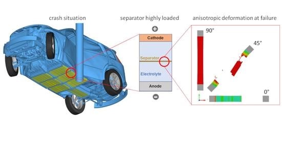
1. Introduction
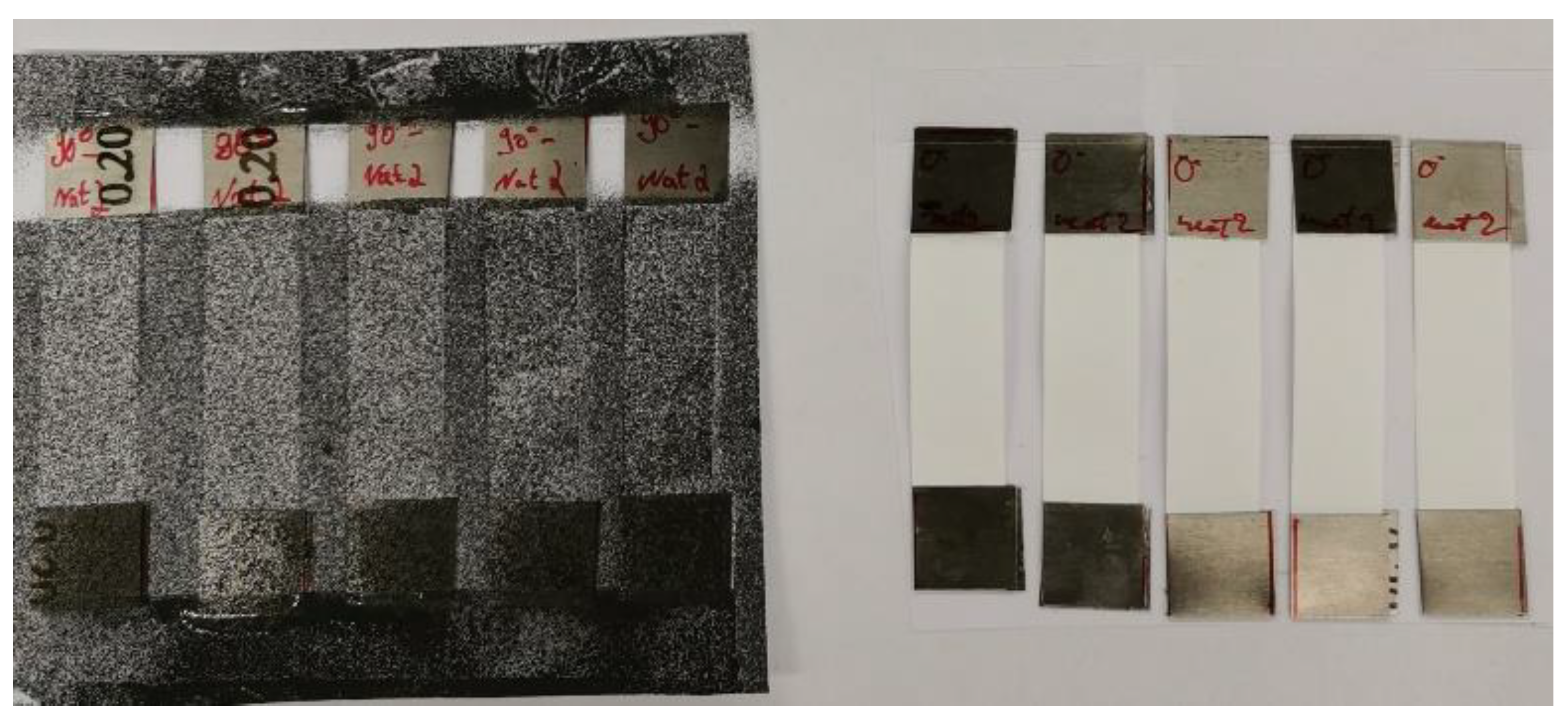
2. Materials and Methods
3. Modeling and Results
3.1. Material Modeling
- 1.
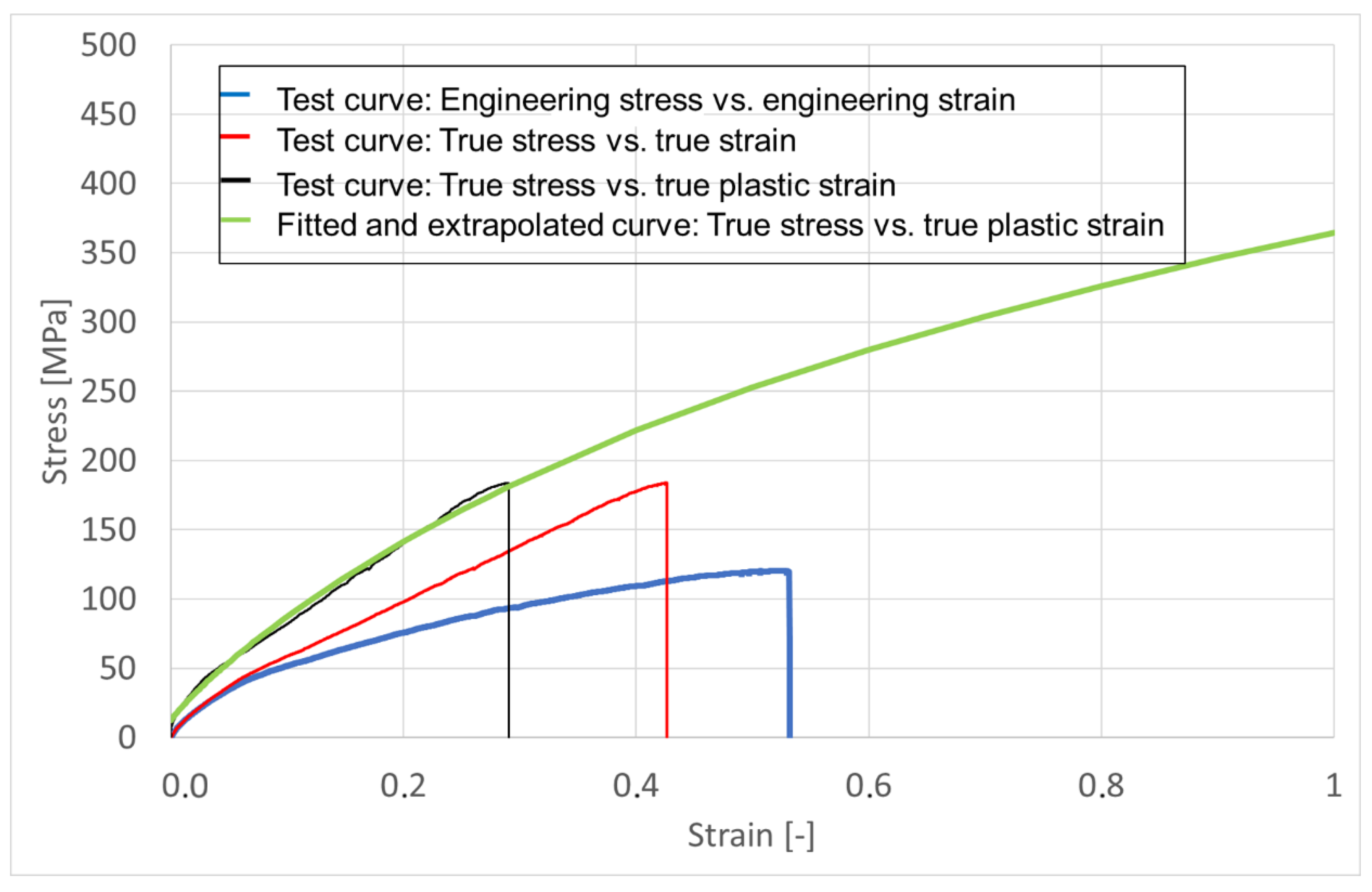
- The resultant force vs. displacement curves are recalculated to engineering stress vs. strain curves. The engineering stress is defined as
- 2.
- In the next step, it is necessary to calculate the true strain from the engineering strain within the parallel length of the test specimen
- 3.
- With the assumption of constant volume (i.e., isochoric deformation), the true stress is the ratio of the measured force F and the actual cross section S:
- 4.
- For use in FEM applications, where the total true stain is the sum of the plastic strain and the elastic strain, the true plastic strain
- 5.
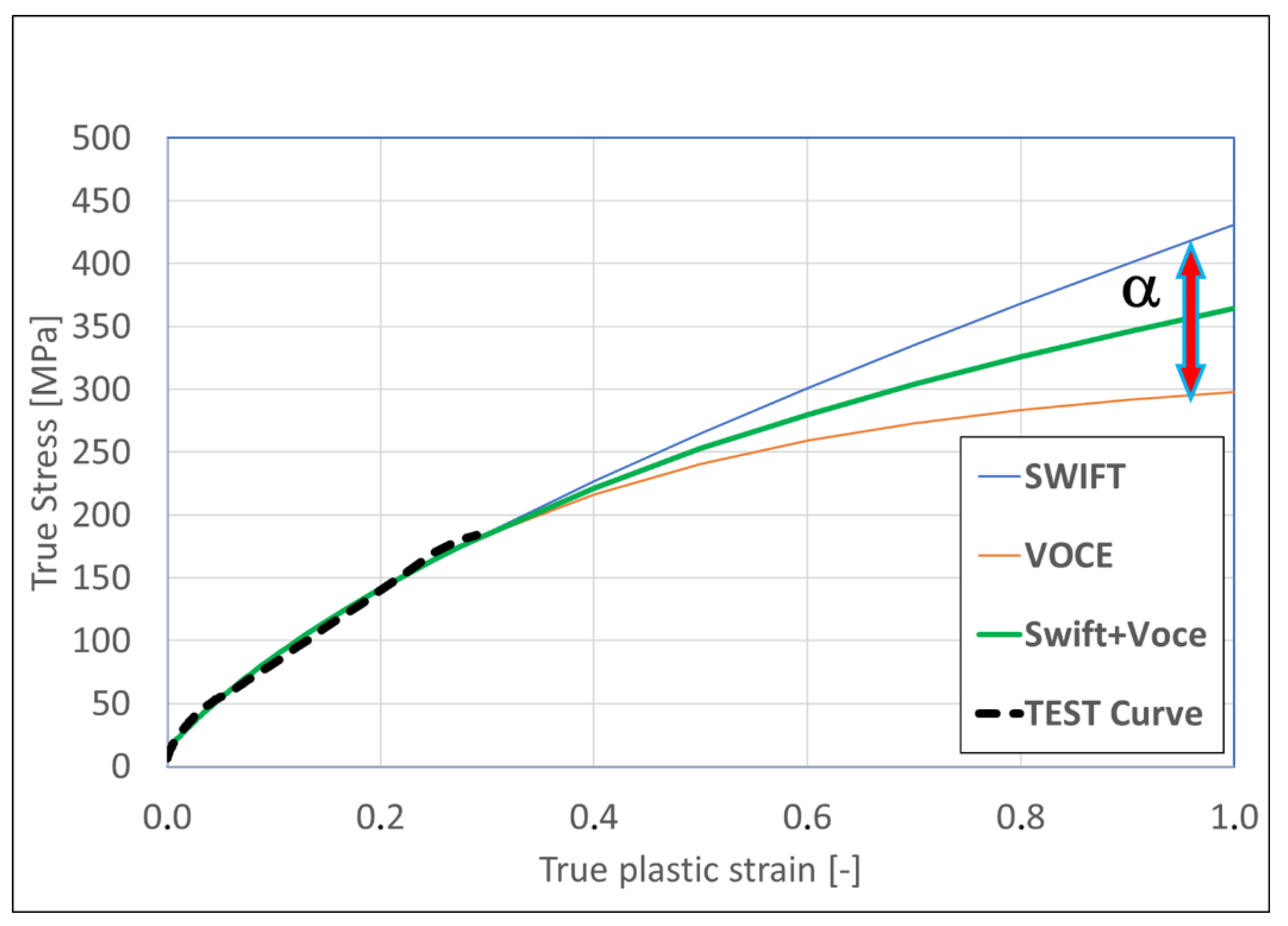
- As the measured data are coming from a tensile test, it shows softening after reaching the maximum stress, where the slope of the stress-strain curve becomes zero or negative. This is often referred to as the necking or instability point. In more complex load scenarios, other load-states can occur, like shear or compression, and the obtained curve can go beyond that point. In the present work, the extrapolation based on the combined equations from Swift and Voce [18] is found as a suitable extrapolation approach for the measured true stress vs. true strain curves:
3.2. Failure Criterion Modeling
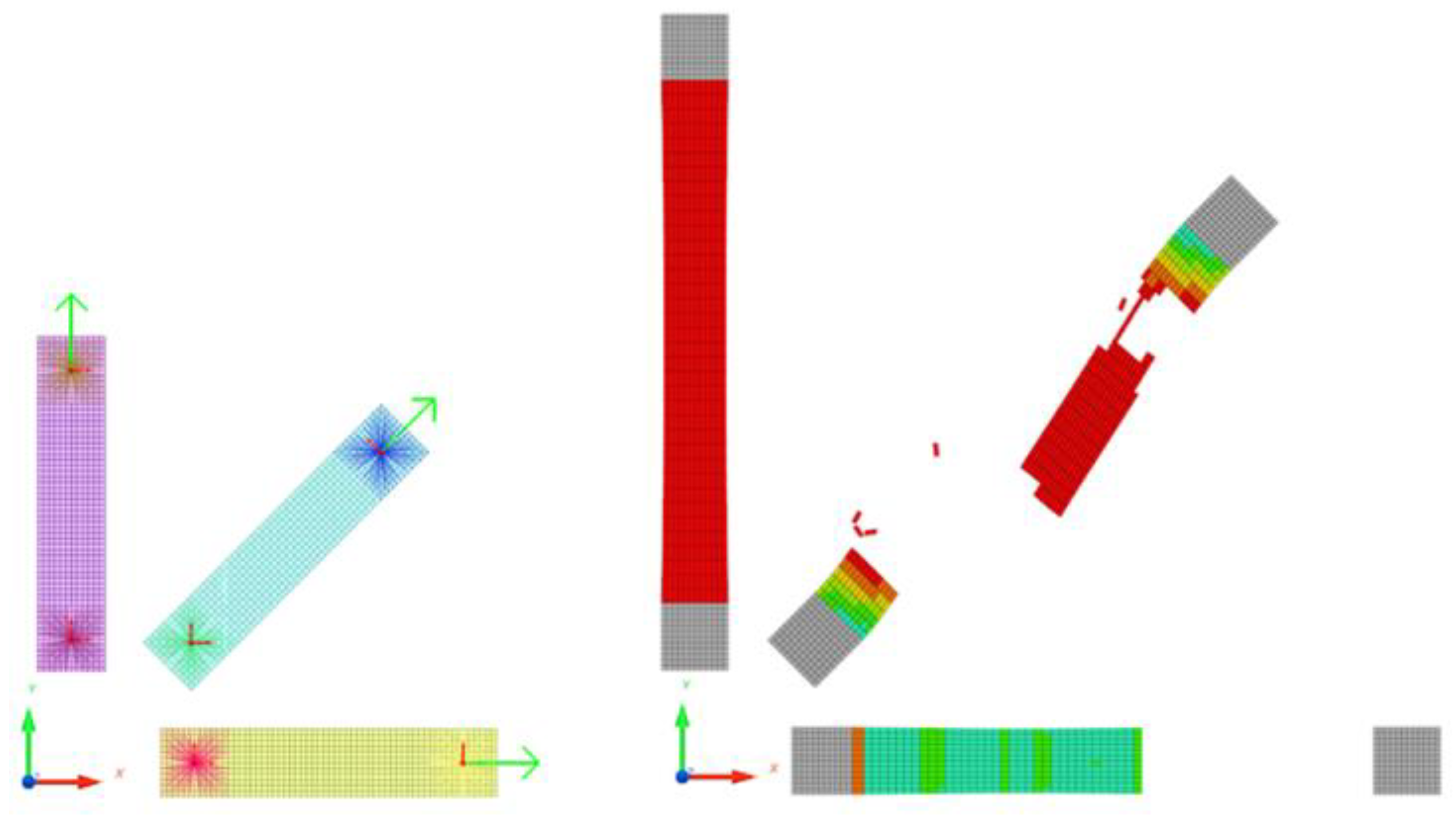
3.3. FE-Model
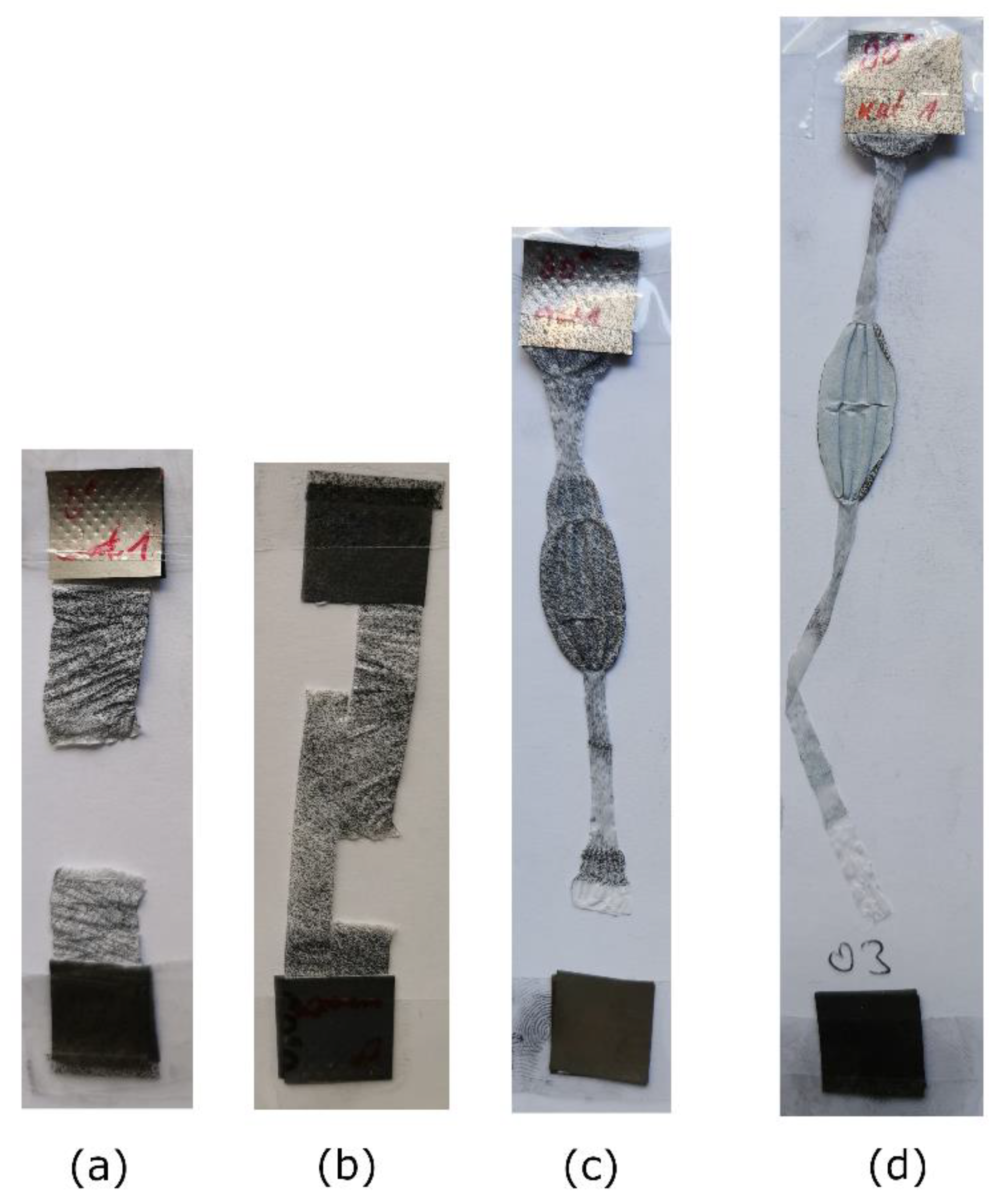
- 0° with failure strain = 53%;
- 45° with failure strain = 95%;
- 90° with failure strain = 120%.
4. Discussion
5. Conclusions and Outlook
Author Contributions
Funding
Acknowledgments
Conflicts of Interest
References
- Koerver, R.; Zhang, W.; de Biasi, L.; Schweidler, S.; Kondrakov, A.O.; Kolling, S.; Brezesinski, T.; Hartmann, P.; Zeier, W.G.; Janek, J. Chemo-mechanical expansion of lithium electrode materials–on the route to mechanically optimized all-solid-state batteries. Energy Environ. Sci. 2018, 11, 2142–2158. [Google Scholar] [CrossRef]
- Vehicles—Department of Energy: Energy.gov. Available online: https://www.energy.gov (accessed on 3 May 2014).
- Hillmann, J. The New Golf VII—Lightweight Design in Large Scale Production; Conference Contribution Aachener Karosserietage: Aachen, Germany, 2012. [Google Scholar]
- US Traffic Watchdog Takes Tesla to Task by Mike Ramsey. Available online: http://www.wsj.com/ (accessed on 19 November 2013).
- Johnson, G.R.; Cook, W.H. A constitutive model and data for metals subjected to large strains, high strain rates and high. In Proceedings of the 7th International Symposium on Ballistics, The Hague, The Netherlands, 19–21 April 1983; pp. 541–547. [Google Scholar]
- Wierzbicki, T.; Bao, Y.; Lee, Y.W.; Bai, Y. Calibration and evaluation of seven fracture models. J. Mech. Sci. 2005, 47, 719–743. [Google Scholar] [CrossRef]
- Sahraei, E.; Meier, J.; Wierzbicki, T. Characterizing and modeling mechanical properties and onset of short circuit for three types of lithium-ion pouch cells. J. Power Sources 2014, 247, 503–516. [Google Scholar] [CrossRef]
- Sahraei, E.; Campbell, J.; Wierzbicki, T. Modeling and short circuit detection of 18650 Li-ion cells under mechanical abuse conditions. J. Power Sources 2012, 220, 360–372. [Google Scholar] [CrossRef]
- Creve, L.; Fehrenbach, C. Mechanical testing and macro-mechanical finite element simulation of the deformation, fracture, and short circuit initiation of cylindrical Lithium ion battery cells. J. Power Sources 2012, 214, 377–385. [Google Scholar] [CrossRef]
- Zhu, F.; Bulla, M.; Lei, J.; Du, X.; Currier, P.; Sypeck, D. Experimental and computational study on the failure behavior of vehicle battery modules subject to wedge cutting. In Proceedings of the ASME international congress, Salt Lake City, UT, USA, 11–13 November 2019. [Google Scholar]
- Yan, S.; Deng, J.; Bae, C.; He, Y.; Asta, A.; Xiao, X. In-plane orthotropic property characterization of a polymeric battery separator. J. Polym. Test. 2018, 46–54. [Google Scholar] [CrossRef]
- Xie, W.; Liu, W.; Dang, Y. Multi-scale modelling of the tensile behavior of lithium ion battery cellulose separator. Polym. Int. 2019, 68, 1341–1350. [Google Scholar] [CrossRef]
- Yan, S.; Deng, J.; Bae, C.; Kalnanus, S.; Xiao, X. Orthotropic Viscoelastic Modeling of Polymeric Battery Separator. J. Electrochem. Soc. 2020. [Google Scholar] [CrossRef]
- Zhu, J.; Li, W.; Wierzbicki, T.; Xia, Y.; Harding, J. Deformation and failure of lithium-ion batteries treated as a discrete layered structure. J. Plast. 2019. [Google Scholar] [CrossRef]
- Altair Engineering, Inc. RADIOSS Manual, USA. 2018. Available online: www.altairhyperworks.com (accessed on 17 March 2020).
- Zhang, X.; Sahraei, E.; Wang, K. Li-ion Battery Separators, Mechanical Integrity and Failure Mechanisms Leading to Soft and Hard Internal Shorts. Sci. Rep. 2016, 6, 32578. [Google Scholar] [CrossRef] [PubMed]
- National Highway Traffic Safety Administration. Available online: https://www.nhtsa.gov/crash-simulation-vehicle-models (accessed on 3 March 2018).
- Roth, C.; Mohr, D. Effect of strain rate on ductile fracture initiation in advanced high strength steel sheets: Experiments and modeling. J. Plast. 2014, 56, 19–44. [Google Scholar] [CrossRef]
- Bulla, M. Failure Criteria for Explicit Analysis in Altair—RADIOSS. In Proceedings of the Altair Technology Conference, Paris, France, 16–18 October 2018. [Google Scholar]
- Zhang, X.; Sahraei, E.; Kai, W. Deformation and failure characteristics of four types of lithium-ion battery separators. J. Power Sources 2016, 327, 693–791. [Google Scholar] [CrossRef]
- Johnson, G.R.; Cook, W.H. Fracture characteristics of three metals subjected to various strains, strain rates, temperatures and pressures. Eng. Fract. Mech. 1985, 21, 31–48. [Google Scholar] [CrossRef]
- Interpolation Methods. Available online: https://wiki.delphigl.com/index.php/Interpolation (accessed on 17 March 2020).
- MinGW Minimalist GNU for Windows. Available online: http://www.mingw.org/ (accessed on 22 October 2018).
- Pfeiffer, M.; Kolling, S. A constitutive model for the anisotropic elastic–plastic deformation of paper and paperboard. J. Solids Struct. 2019, 39, 4053–4071. [Google Scholar]


| Swift: A (MPa) | Swift: eps0 (-) | Swift: n (-) | Voce: k0 (MPa) | Voce: Q (MPa) | Voce: B (-) |
|---|---|---|---|---|---|
| 429.255 | 5.32 × 10⁻³ | 0.7071 | 14.544 | 303.095 | 2.741 |
| Orientation (degree) | Uniaxial Compression (-) | Pure Shear (-) | Uniaxial Tension (-) | Plain Strain Tension (-) | Equi-Biaxial Tension (-) |
|---|---|---|---|---|---|
| 0 | 1.0 | 0.75 | 0.53 | 0.50 | 0.7 |
| 45 | 2.5 | 1.35 | 0.95 | 0.60 | 0.8 |
| 90 | 4.0 | 1.85 | 1.20 | 0.70 | 0.9 |
| Orientation (degree) | Displacement at Failure in Test (mm) | Displacement at Failure in Simulation (mm) |
|---|---|---|
| 0 | 19.1 | 18.9 |
| 45 | 34.2 | 33.5 |
| 90 | 43.2 | 44.2 |
© 2020 by the authors. Licensee MDPI, Basel, Switzerland. This article is an open access article distributed under the terms and conditions of the Creative Commons Attribution (CC BY) license (http://creativecommons.org/licenses/by/4.0/).
Share and Cite
Bulla, M.; Kolling, S.; Sahraei, E. An Experimental and Computational Study on the Orthotropic Failure of Separators for Lithium-Ion Batteries. Energies 2020, 13, 4399. https://doi.org/10.3390/en13174399
Bulla M, Kolling S, Sahraei E. An Experimental and Computational Study on the Orthotropic Failure of Separators for Lithium-Ion Batteries. Energies. 2020; 13(17):4399. https://doi.org/10.3390/en13174399
Chicago/Turabian StyleBulla, Marian, Stefan Kolling, and Elham Sahraei. 2020. "An Experimental and Computational Study on the Orthotropic Failure of Separators for Lithium-Ion Batteries" Energies 13, no. 17: 4399. https://doi.org/10.3390/en13174399
APA StyleBulla, M., Kolling, S., & Sahraei, E. (2020). An Experimental and Computational Study on the Orthotropic Failure of Separators for Lithium-Ion Batteries. Energies, 13(17), 4399. https://doi.org/10.3390/en13174399