A Proposal for an MPPT Algorithm Based on the Fluctuations of the PV Output Power, Output Voltage, and Control Duty Cycle for Improving the Performance of PV Systems in Microgrid

Abstract

In microgrids, distributed generators that cannot be dispatched, such as a photovoltaic system, need to control their output power at the maximum power point. The fluctuation of their output power should be minimized with the support of the maximum power point tracking algorithm under the variation of ambient conditions. In this paper, a new maximum power point tracking method based on the parameters of power deviation ($\Delta P_{PV}$), voltage difference ($\Delta V_{PV}$), and duty cycle change ($\Delta D$) is proposed for photovoltaic systems. The presented algorithm achieves the following good results: (i) when the solar radiance is fixed, the output power is stable around the maximum power point; (ii) when the solar radiance is rapidly changing, the generated power is always in the vicinity of maximum power points; (iii) the effectiveness of energy conversion is comparable to that of intelligent algorithms. The proposed algorithm is presented and compared with traditional and intelligent maximum power point tracking algorithms on the simulation model by MATLAB/Simulink under different radiation scenarios to prove the effectiveness of the proposed method.

1. Introduction

The Microgrid (MG) is currently the grid structure of interest as it is capable of integrating multiple distributed energy resources, especially renewable ones, which significantly reduces concerns about climate changes. In an MG, the generated power sources are located close to the loads, and hence, it should lessen the capacity of transmission power systems. As a result, this increases the reliability and improves the power quality while lessening infrastructure requirements and power transmission and reducing emission and generation costs.

However, the applications of renewable energy sources pose several challenges arising from their dependent uncertainty factors (the output capacity depends heavily on weather conditions) and the variation of loads. The most common renewable energy sources are hydroelectric, solar, and wind. Although hydroelectricity is predominant, Photovoltaic (PV) energy sources are increasing more than 30% per year [1]. The power grid with a high penetration of PV sources results in a power imbalance, along with the related issues of power quality and reliability as PV sources have intermittent and non-linear characteristics. Their properties and output power variation depend greatly on environmental factors. Therefore, there have been many studies [2,3,4,5] to enhance the efficiency of MG by improving the working efficiency of the PV system.

Several mathematical models of a PV panel have been developed in the literature [6,7,8,9,10,11,12,13,14,15]. Among them, the single-diode equivalent-circuit model, which is shown in Figure 1, is the most widely used for presenting the operation of a PV cell [12,13,14,15]. This PV model consists of a DC current source $I_{ph}$, a diode D, a resistance $R_{sh}$ connected in parallel with this current source, and a series resistance $R_s$. The current source $I_{ph}$ represents the PV current of the cell, which is directly proportional to the solar irradiance G. The parallel resistance $R_{sh}$ illustrates the leakage current, and the series resistance $R_s$ represents the Ohmic losses.

By applying this equivalent model, a PV array under specific solar radiance and temperature has a current ($I_{PV}$)–voltage ($V_{PV}$) characteristic as shown in Figure 2. This characteristic curve has an exclusive point, called the Maximum Power Point (MPP). When operating at this point, the PV array generates the maximum output power and reaches the optimal performance. If a PV array is directly connected to a load, the operating point will be the intersection of the $I_{PV}-V_{PV}$ characteristic of the PV array and the load line as illustrated in Figure 2. It can be seen from Figure 2 that this operating point is not located at the PV array’s MPP. In addition, it is also strongly affected by the solar radiance and PV temperature levels [16,17]. Therefore, the PV array must be designed in an over-sized manner to ensure that it can supply the full load’s power requirements. Consequently, this results in an expensive cost for the PV system’s construction.

Thus, in order to dynamically set the MPP as the operating point of a PV array for a wide range of solar irradiation and temperature, specific circuits, known as Maximum Power Point Tracking (MPPT) circuits [18,19], are integrated between the PV module and loads, as shown in Figure 3. The MPPT operation aims to control the PV array’s voltage or current independently of the load’s parameters. If a suitable algorithm is applied, the MPPT can locate and track the MPP of the PV array. The aim of MPPT algorithms is to continuously adjust the operating point of the PV array to keep it as close as possible to the MPP under various conditions of weather or load demand. Hence, MPPT techniques can improve the PV system’s performance and reduce the total system cost.

Multiple MPPT techniques have been developed and improved in the literature and widely used in practice, such as Perturb and Observe (P&O), Incremental Conductance (INC), and Hill Climbing (HC) [20,21,22,23,24,25]. In general, they aim to quickly track the MPP operation point under such continuously changing conditions and generate small output power fluctuation. However, the fast tracking response and accuracy conflict with each other, so these tracking methods cannot meet both of them [22]. During the steady-state operation, the fluctuation of output power around the MPP can be minimized by reducing the increment duty cycle step size in these methods. However, a smaller value of the step size will slow down the convergence speed of the MPPT controller, especially under the rapid change of weather conditions [22]. To overcome this drawback, several adaptive control algorithms based on these MPPT methods were suggested by utilizing the variable perturbation during tracking processes [3,26,27,28]. Although these proposals present better performance compared to a fixed perturbation parameter, they are still not truly accurate and fast as the impacts of ambient conditions have not been considered thoroughly [3].

In order to overcome the limitations of the above traditional MPPT algorithms, some intelligent MPPT methods based on Fuzzy Logic (FL) and Artificial Neural Network (ANN) have been proposed [23,29,30,31,32,33]. However, these suggestions contain some drawbacks, such as complexity, high cost, the requirement of high-performance micro-processor, and in some cases, the employment of extra sensors for ambient conditions. In detail, the FL control model is based on fuzzy rules, which consist of three major operations: fuzzification, inference, and defuzzification. The collected data are put into an FL-based system where the input quantities are transferred to linguistic variables with appropriate membership functions. If the defined membership function is increased, the associated computational process increases as well [23,29,30,31]. In terms of ANN, it is an artificial intelligence method that has more advantages than conventional MPPT methods [32]. However, the controller needs much information to train the neurons present in the algorithm, and it is usually implemented in combination with other conventional MPPT methods [32]. To employ ANN or FL techniques, the designer must have significant knowledge of the operation of each PV system [19,29,31]. Therefore, these intelligent MPPT methods are merely spread in practical PV applications.

In this paper, the suggested MPPT method is based on three main factors: (i) the variation of the PV’s output power; (ii) the variation of the output voltage; and (iii) the change of the duty cycle of the MPPT controller. By utilizing these fundamental parameters in combination, the proposed technique presents significant advantages as follows:

• Simplicity in implementation because of the fundamental measured parameters ($\Delta P_{PV}$, $\Delta V_{PV}$, and $\Delta D$);
• Accuracy and almost no oscillation around the MPP during tracking and steady-state operations;
• The necessary requirements of an MPPT technique are achievable by using only a low-cost controller due to the simplicity of the proposed algorithm;
• Unaffected by the fixed perturbation value (increment size of the duty cycle) for a wide range of this parameter.

The paper is organized as follows: Following the Introduction in Section 1, Section 2 is reserved for the detailed reviews of three MPPT algorithms, P&O, HC, and MPPT based on FL. The operating principle and structure of the proposed MPPT algorithm are presented in Section 3. In Section 4, some simulation results are shown to validate the advantages of this proposed MPPT method. Finally, a brief summary of this paper is given in Section 5.

2. Review of MPPT Algorithms

Numerous MPPT techniques have been introduced in the literature; this section only provides a review of the three common methods utilized in most of PV systems, which are the P&O algorithm, the HC algorithm, and the MPPT algorithm based on FL. The details of these techniques are discussed in this section.

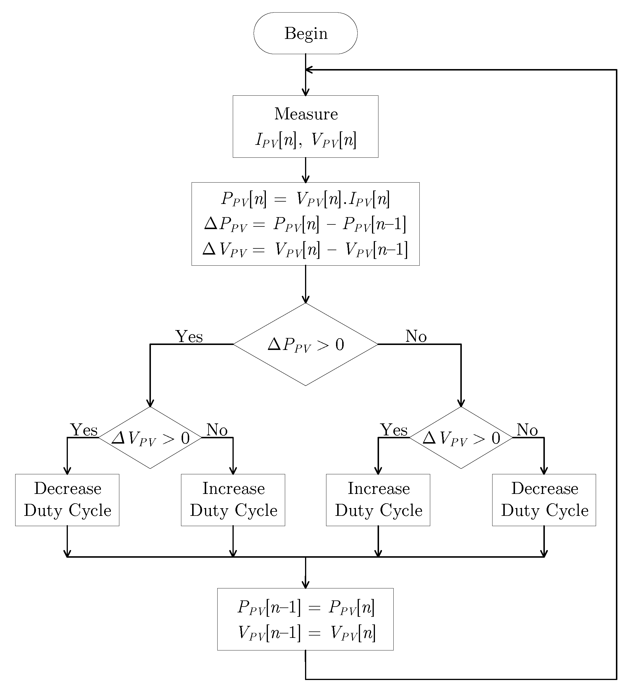
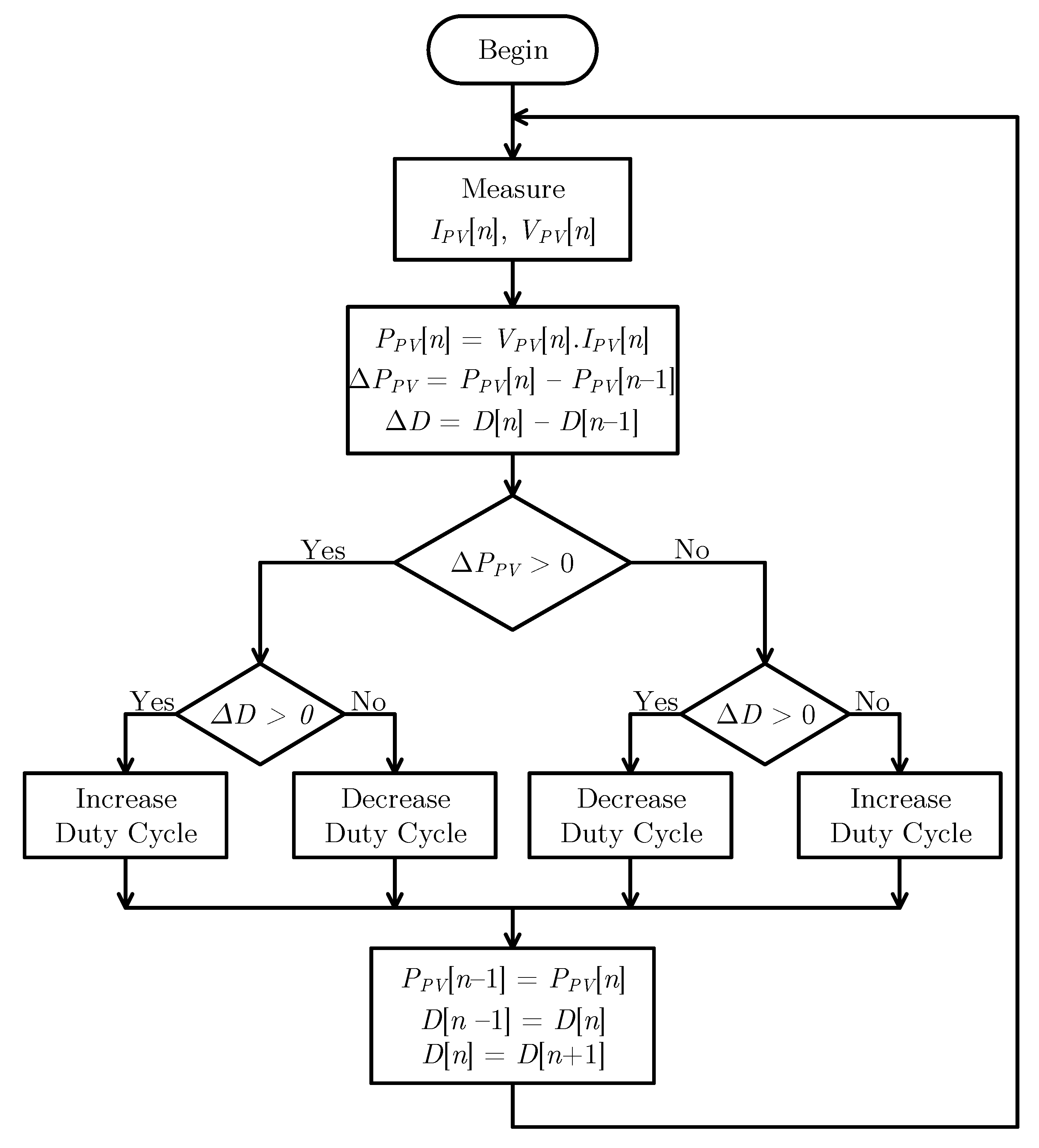
2.1. Perturb and Observe Algorithm

The most basic form of the P&O algorithm was presented in [22,23,24]. The P&O algorithm is periodically carried out by perturbing the operating voltage and observing the power variation in order to regulate the operating point to move toward the MPP. The voltage perturbation for the MPP tracking is carried out by decreasing or increasing the duty cycle of the MPPT controller by a small value ($D_{step}$) in each control period. The algorithm can be easily understood by the following flowchart, which is shown in Figure 4.

Nevertheless, a general drawback of the P&O algorithm is that the operating point fluctuates around the MPP at the steady state, and therefore, this results in the loss of the PV system’s energy. Moreover, the larger the duty cycle step ($D_{step}$), the more power oscillation occurs. In order to reduce the oscillations around the MPP in the steady state, the duty cycle step should be chosen with a smaller value. However, in that case, it also slows down the speed of response of the MPPT system to the fast change of the atmospheric conditions and reduces the efficiency of the MPPT algorithm [23,24,25]. This drawback is illustrated in Figure 5, where the paths of the operating point with the P&O algorithm under solar radiance variation from 200 W/m${}^2$ are presented. The figure shows two different responses of the PV array in the power and voltage coordinates with the P&O algorithm. The red dotted line in Figure 5 shows the trajectory of the operating point under slowly changing radiance, while the blue continuous one shows the wrong tracking path of the P&O algorithm under the rapid changing of radiance. This failure in the MPP tracking of the P&O algorithm during the period of rapidly increasing radiance can be explained as follows. At the moment solar irradiation starts increasing suddenly, the operating point moves from A to B (in accordance with $\Delta P_{PV}>0$ and $\Delta V_{PV}>0$). According to the P&O algorithm, the controller sends signals to decrease the duty cycle D to increase the operating voltage. On the contrary, the duty cycle D is increased due to the P&O algorithm when the operating point moves from B to C (in accordance with $\Delta P_{PV}>0$, $\Delta V_{PV}<0$, and $\Delta D<0$). As a result, the operating point continues moving from C to D. As the irradiation increases, the signal’s width D continues widening in the following cycles, and thus, the operating point moves toward E until the irradiation stops rising.

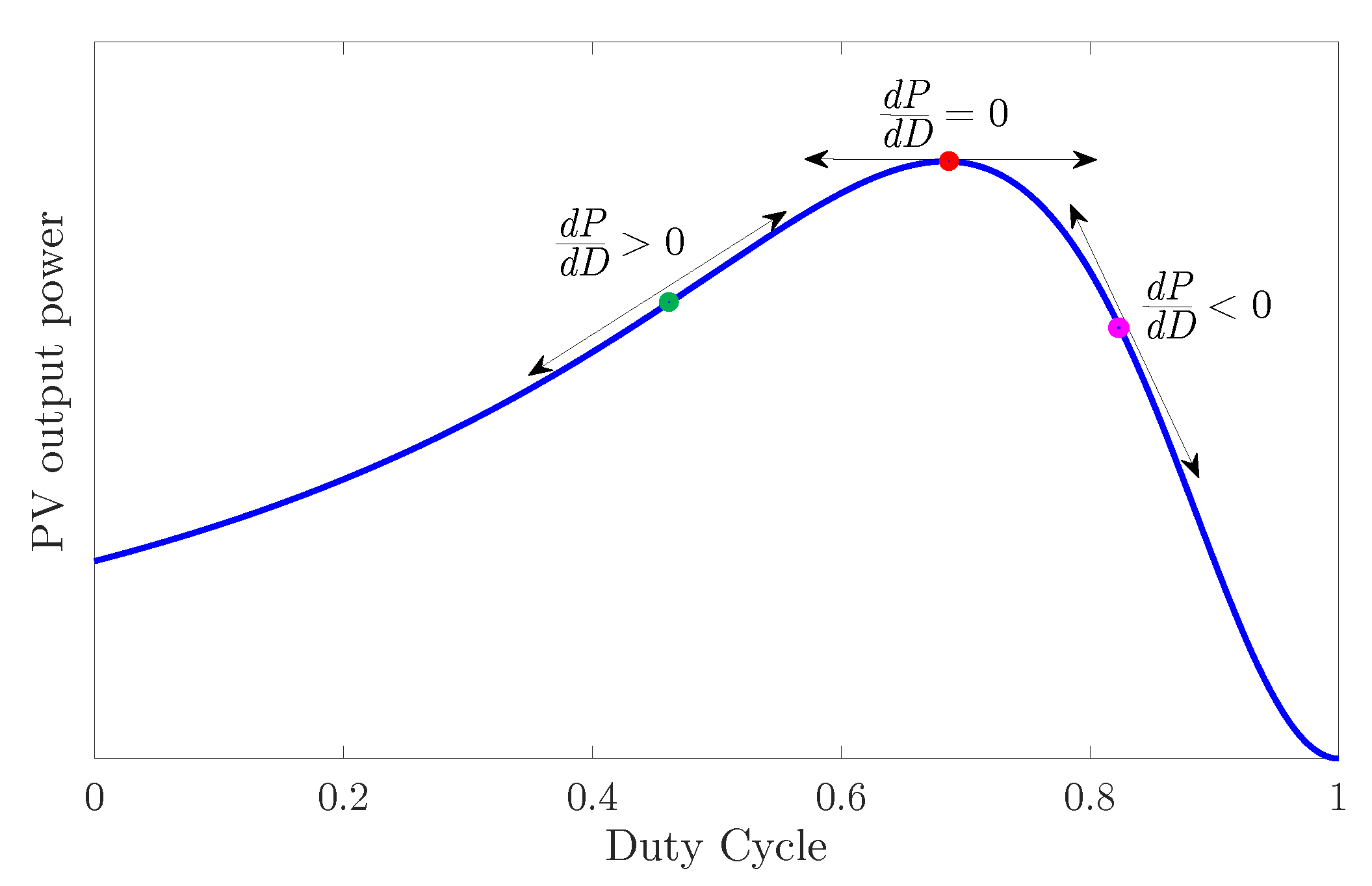
2.2. Hill Climbing Algorithm

In a PV system’s MPPT structure, as in Figure 3, a power electronic DC/DC converter is used as the interface connection between the PV array and loads. The control parameter of the power electronics stage is the switching duty cycle of the PWM signal of the MPPT controller. Therefore, another approach to maximize the output power of the PV system is based on the relationship curve between the PV system output power and the PWM duty cycle [21,22]. Figure 6 shows a typical hill-shaped PV array output power curve with respect to the PWM duty cycle, where $P_{PV}$ is the PV array output power and D represents the PWM duty cycle of a DC/DC boost converter [21]. There is a unique value of the duty cycle at which the output power of the PV array reaches the maximum level. The flowchart of the control algorithm is shown in Figure 7.

The advantage of the HC MPPT algorithm is its simplicity. Furthermore, the MPP can be tracked accurately when the solar irradiance increases rapidly [21]. However, it is only effective in the case of using a small value of the duty cycle steps. Otherwise, the level of oscillating power around the MPP is very large.

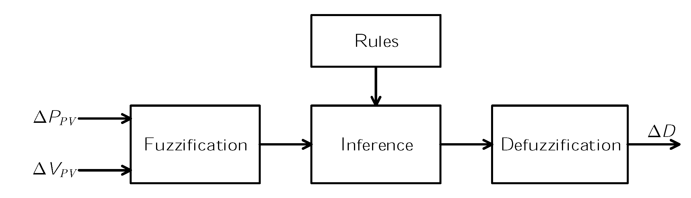
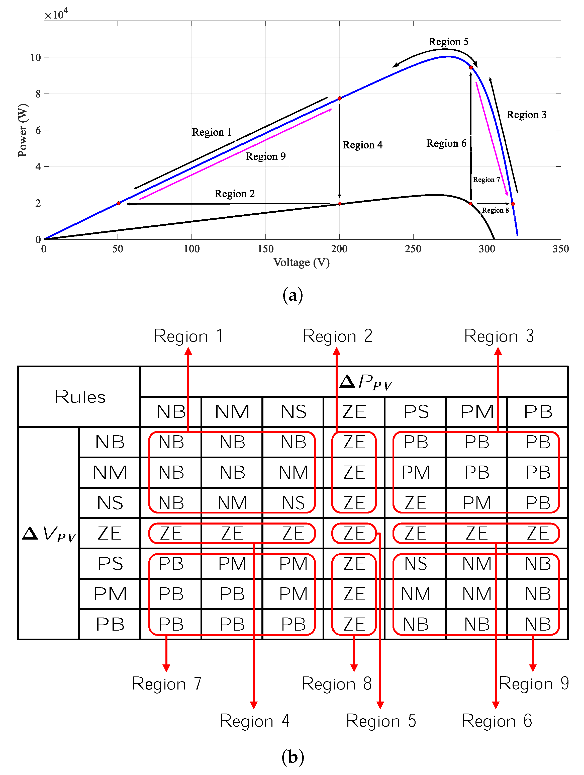
2.3. Fuzzy Logic Based MPPT Algorithm

FL is one of the intelligent control methods and is applied in many fields of control theory. The fuzzy controller is able to receive and process unstable and complex data, fix bugs, and offer optimal solutions to make control objects perform better. FL provides a methodology that can integrate human-like thinking into a control system.

There are three stages in an FL control algorithm as shown in Figure 8, namely fuzzification, inference, and defuzzification [34].

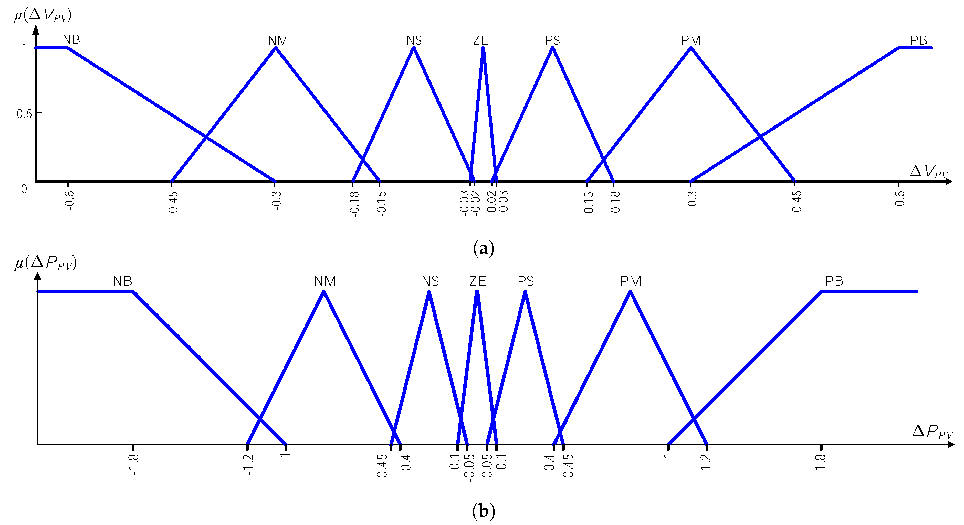
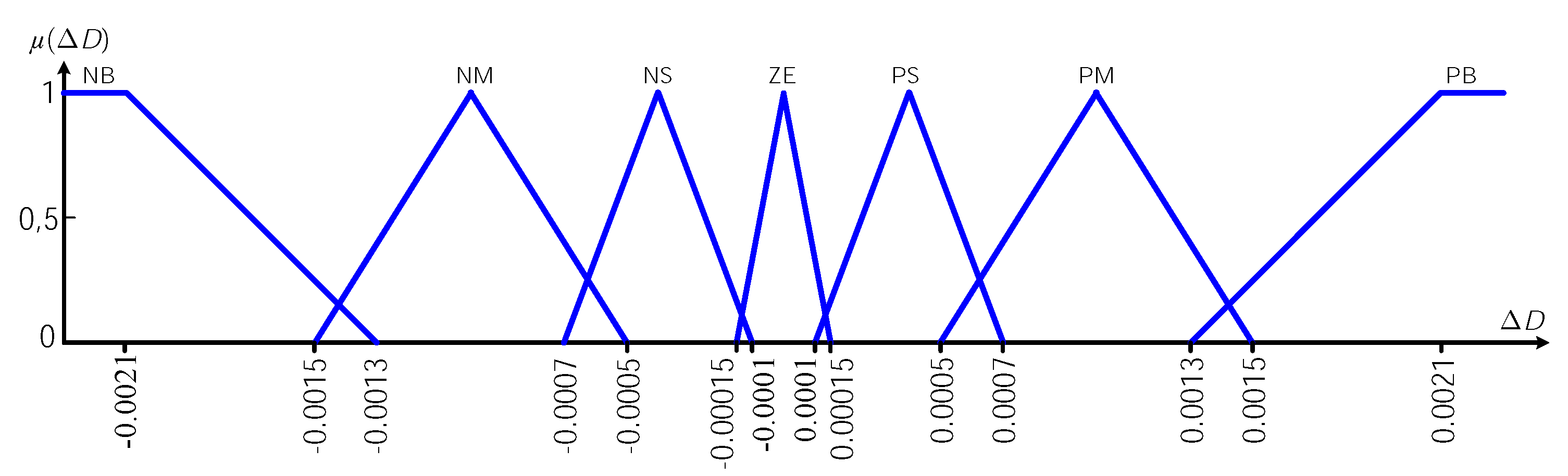
2.3.1. Fuzzification

Fuzzification is the process of turning numerical variables into fuzzy variables. The actual voltage and current of a PV array can be continuously measured and used to calculate the power [23]. The input data of the considered FL controller are $\Delta V_{PV}$ and $\Delta P_{PV}$. These input variables are defined as follows:

$$\begin{array}{cc}\hfill \Delta V_{PV}& =V_{PV}\left[k\right]-V_{PV}[k-1],\hfill \end{array}$$

(1)

$$\begin{array}{cc}\hfill \Delta P_{PV}& =P_{PV}\left[k\right]-P_{PV}[k-1].\hfill \end{array}$$

(2)

where $V_{PV}\left[k\right]$ and $P_{PV}\left[k\right]$ are respectively the power and voltage deviation of the PV array at time k.

The set of input parameters is described by the set NB, NM, NS, ZE, PS, PM, PB, where NB (Negative Big) is a large decrease, NM (Negative Moderate) is a moderate decrease, NS (Negative Small) is a small decrease, ZE (zero) is no increase or decrease, PS (Positive Small) is a small increase, PM (Positive Moderate) is a moderate increase, and PB (Positive Big) is a large increase. Figure 9a,b shows the membership functions of the seven basic fuzzy subsets for the input variables.

2.3.2. Inference

The relationship between the output voltage and the input voltage of DC/DC boost converters is as follows:

$$V_{out}={\displaystyle \frac{V_{in}}{1-D}}={\displaystyle \frac{V_{PV}}{1-D}}.$$

(3)

As $V_{out}$ is kept constant, $V_{in}$ is inversely proportional to the duty cycle D.

Based on the $P_{PV}-V_{PV}$ characteristic curve of the PV panel in Figure 10a, the fuzzy control rule can be inferred. The properties of the panel are divided into nine regions [34]. Based on the relationship between voltage deviation and power deviation, as well as the fuzzy sets of input and output, the fuzzy controller is designed to use the control rule as shown in Figure 10b.

2.3.3. Defuzzification

The set of output parameters is described by the set NB, NM, NS, ZE, PS, PM, PB, where NB is a large decrease, NM is a moderate decrease, NS is a small decrease, ZE is no increase or decrease, PS is a small increase, PM is a moderate increase, and PB is a large increase. Figure 11 shows the membership functions that correspond to the relevant output variable $\Delta D$.

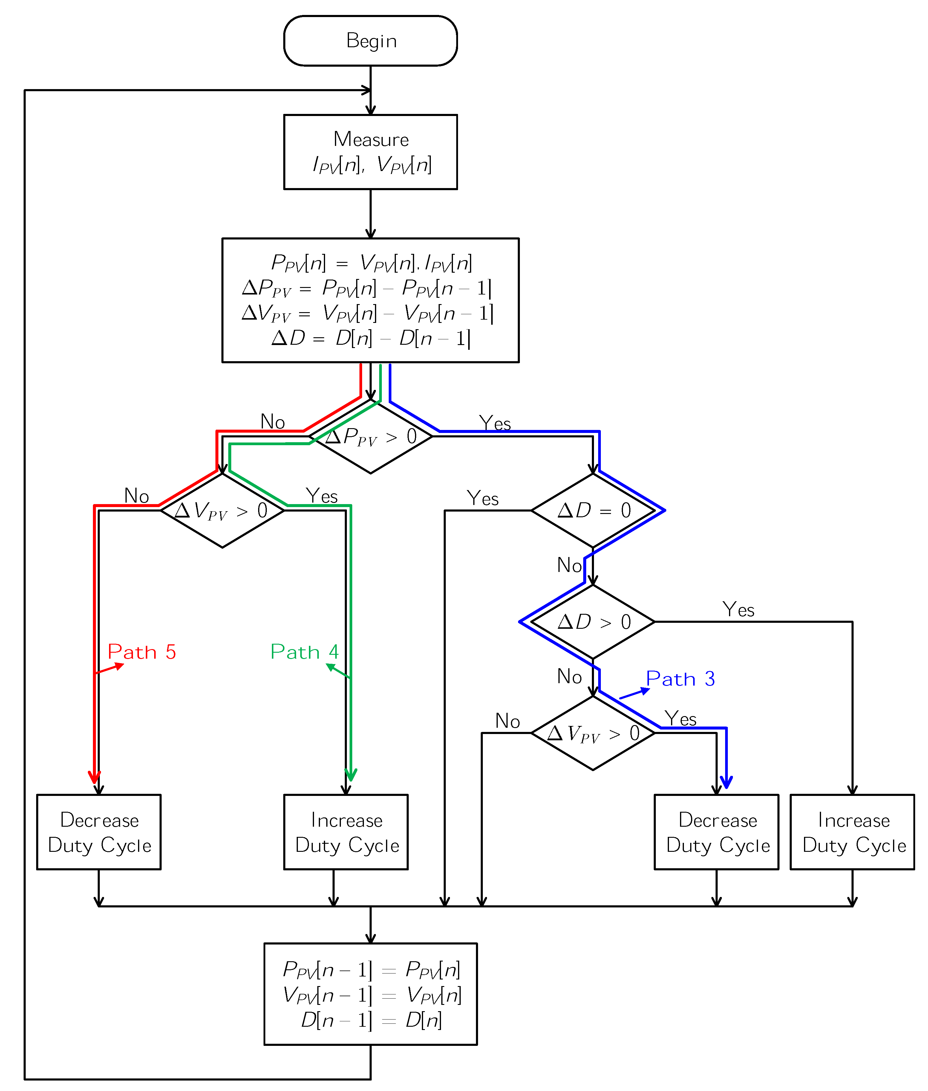
3. Proposed MPPT Algorithm

The flowchart of the proposed MPPT method is shown in Figure 12. This method is changed based on the P&O and HC algorithms. In the P&O algorithm, the variations of two PV factors, $P_{PV}$ and $V_{PV}$, are considered, whereas the changes of the PWM duty cycle, D and $P_{PV}$, are used to determine the value of the controller’s duty cycle in the next control period in the HC algorithm. In the proposed MPPT algorithm, all three control elements are used to combine the advantages of these two algorithms. The proposed algorithm aims to track the MPP point correctly either under stable irradiation or suddenly changing radiance.

When the three factors $\Delta V_{PV}$, $\Delta P_{PV}$, and $\Delta D$ are taken into account in the proposed algorithm, its operation in the steady state is explained in detail in the following situations.

3.1. Suddenly Increasing Solar Irradiation

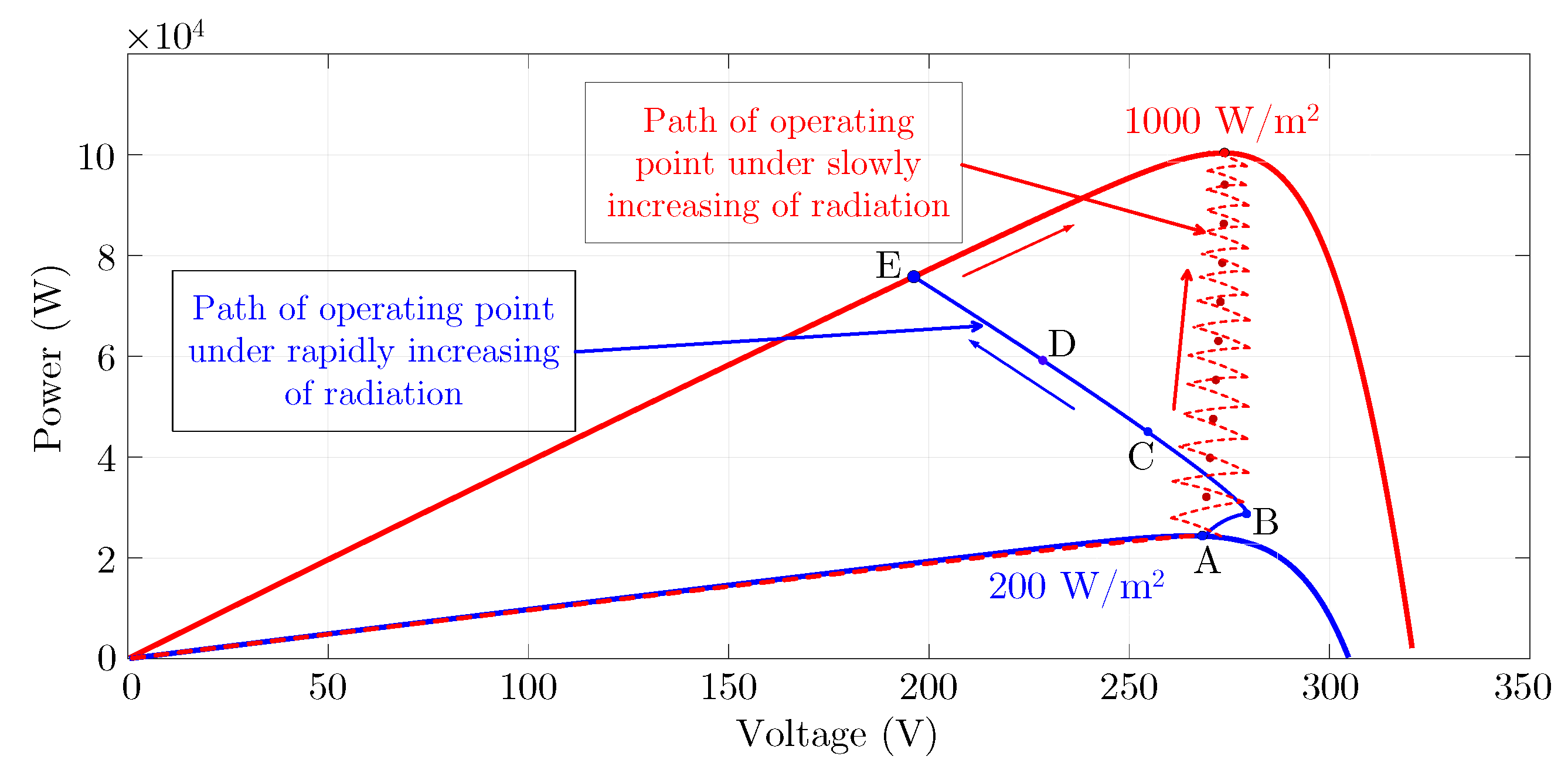
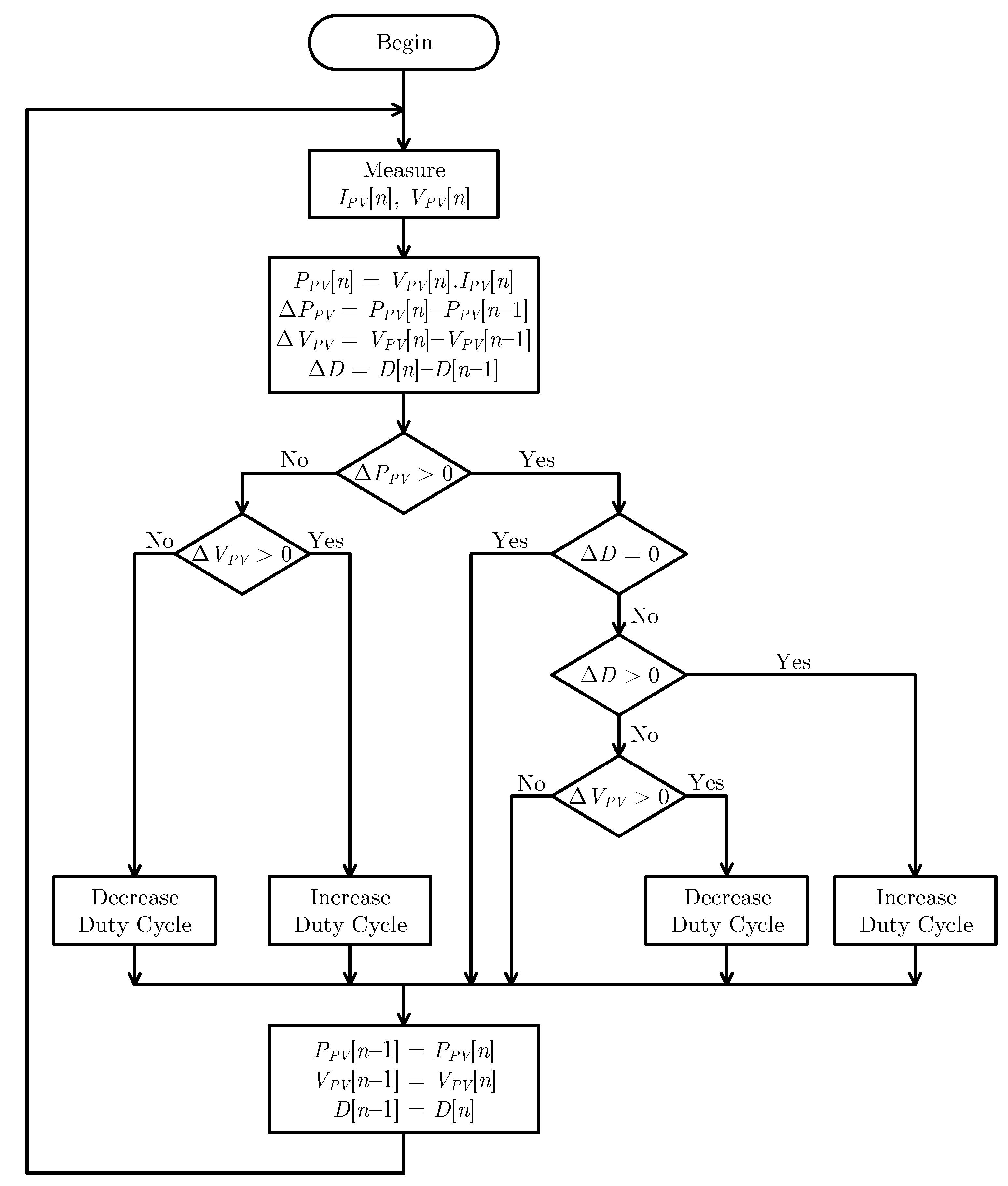
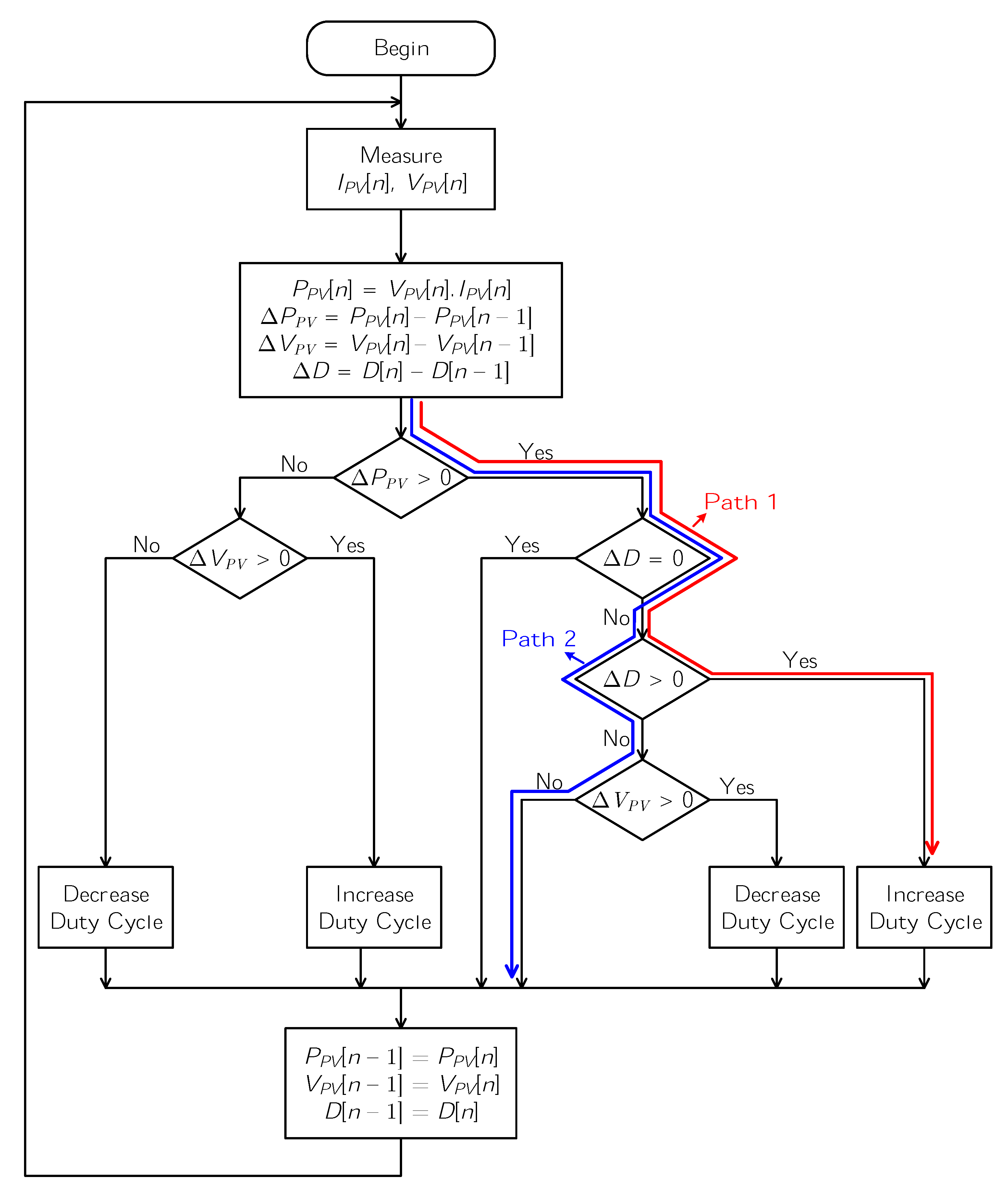
When the solar irradiation increases, the power output of PV systems also increases accordingly ($\Delta P_{PV}>0$). As a result, there are two possibilities to consider.

• In the case of $\Delta P_{PV}>0$ and $\Delta D>0$: The increase of duty cycle D at the current switching cycle causes the rise of the output power. At this moment, the MPPT controller will increase the duty cycle D according to the HC algorithm as $\Delta P_{PV}>0$ and $\Delta D>0$. From [21], when the solar irradiation increases, the duty cycle at the MPP ($D_{MPP}$) is also widened. Hence, the MPP moves to the right of the power and duty cycle plane. The duty cycle D should be increased in the following cycle. This adjustment of D is also applied in the case of stable irradiation [21]. Path 1 in Figure 13 presents the adaptiveness of the proposed method in this case.
• In the case of $\Delta P_{PV}>0$, $\Delta V<0$, and $\Delta D<0$: As mentioned in Section 2.1, the P&O algorithm increases the duty cycle D in the following switching cycles. However, this results in not tracking the MPP correctly when the solar irradiation changes suddenly. Thus, instead of varying the duty cycle D, the proposed method keeps D constant in the following switching cycles. The output power of the PV system will increase due to the rise of solar irradiation at the constant value of D. Path 2 in Figure 13 depicts the adaptiveness of the proposed method in this case.

3.2. Stable Solar Radiation

When the solar irradiance is stable, the duty cycle D is adjusted similarly to how the P&O algorithm does. Paths 3, 4, and 5 in Figure 14 illustrate the adaptiveness of the proposed method in this case.

The proposed MPPT algorithm utilizes three parameters ($\Delta P_{PV}$, $\Delta V_{PV}$, and $\Delta D$), which provide the cases of execution, as shown in

Table 1. Executions of the proposed MPPT algorithm.

$\mathbf{\Delta }{\mathit{P}}_{\mathit{P}\mathit{V}}$	$\mathbf{\Delta }{\mathit{V}}_{\mathit{P}\mathit{V}}$	$\mathbf{\Delta }\mathit{D}$	Execution
$=0$	—	—	$D[n+1]=D\left[n\right]$
$>0$	—	$=0$	$D[n+1]=D\left[n\right]$
$>0$	$>0$	$>0$	$D[n+1]=D\left[n\right]+D_{step}$
$>0$	$<0$	$>0$	$D[n+1]=D\left[n\right]+D_{step}$
$>0$	$>0$	$<0$	$D[n+1]=D\left[n\right]-D_{step}$
$>0$	$<0$	$<0$	$D[n+1]=D\left[n\right]$
$<0$	$>0$	$>0$	$D[n+1]=D\left[n\right]+D_{step}$
$<0$	$>0$	$<0$	$D[n+1]=D\left[n\right]+D_{step}$
$<0$	$<0$	$>0$	$D[n+1]=D\left[n\right]-D_{step}$
$<0$	$<0$	$<0$	$D[n+1]=D\left[n\right]-D_{step}$

.

4. Simulation

In [23], a comparison review of the MPPT algorithms based on FL, improved P&O, and improved INC was presented. The comparison results in this paper showed that the FL algorithm achieved better tracking efficiency and faster response time (or convergent speed) than the other adaptive algorithms.

Moreover, in [33], a comparison table of traditional MPPT algorithms and intelligent MPPT algorithms was introduced. In terms of intelligent MPPT algorithms considered in this table (FL, ANN, genetic algorithm), they had equivalent tracking efficiency, complexity level, response time, and cost. On the other hand, the MPPT method based on FL was easier to integrate into the hardware than the other intelligent algorithms.

For all these reasons, in the simulation section of this paper, the authors only chose the MPPT method based on FL to compare with the proposed MPPT algorithm rather than other adaptive algorithms and intelligent algorithms. Besides, the proposed MPPT algorithm is also compared with the conventional P&O method to clarify its superior performance.

The performances of these methods were evaluated at constant ambient temperature (25 ${}^{\circ }$C ) and in two different cases of the fixed duty cycle step ($D_{step}=3\times {10}^{-4}$ and $D_{step}=3\times {10}^{-3}$).

The solar radiation was programmed to change rapidly or slowly in the four following scenarios. The first case was designed to verify the tracking performance with a rapid rise of solar radiation by 400 W/m${}^2$ within half of a second, which is represented as Case 1 in Figure 15 (from $t=5$ s to $t=5.5$ s and from $t=10$ s to $t=10.5$ s). In the second case, the higher slope ramp function for the solar radiance rapid increase was introduced as Case 2 (from 200 W/m${}^2$ at $t=20$ s to 1000 W/m${}^2$ at $t=20.5$ s). In the two remaining cases, MPPT algorithms were evaluated under a gradual increase and stable solar radiance, as illustrated in Case 3 and Case 4, respectively.

The PV system of the “Average model of a 100-kW Grid-Connected PV Array” in the MATLAB/Simulink environment was employed to perform this investigation. The 100-kW PV array consisted of 66 strings of five series-connected 305.2-W modules connected in parallel ($66\times 5\times 305.2\mathrm{W}=100.7$ kW). The detailed specifications of the PV panel, PV array, and the DC/DC boost converter are given in

Table 2. Characteristics of the PV panel, PV array structure, and DC/DC boost converter parameters.

Panel Data
Module		SunPower SPR-305E-WHT-D
Maximum power (W)	305.226	Cells per module ($N_{cell}$)	96
Open circuit voltage $V_{oc}$ (V)	64.2	Short-circuit current $I_{sc}$ (A)	5.96
Voltage at maximum power point $V_{mpp}$	54.7	Current at maximum power point $I_{mpp}$	5.58
Temperature coefficient of $V_{oc}$ (%/°C)	−0.27269	Temperature coefficient of $I_{sc}$ (%/${}^{\circ }$C)	0.061745
Array Data
Parallel strings		66
Series-connected modules per string		5
Maximum power (kW)		100.7
Temperature ${}^{\circ }$C		25
Boost Converter’s Parameters
Inductor L		0.64 mH
Output capacitor $C_o$		100 $\mathsf{\mu }$F
Initial duty cycle		0.5
Duty cycle step $D_{step}$		$3\times {10}^{-4}÷3\times {10}^{-3}$
Switching frequency $f_{sw}$		50 kHz

.

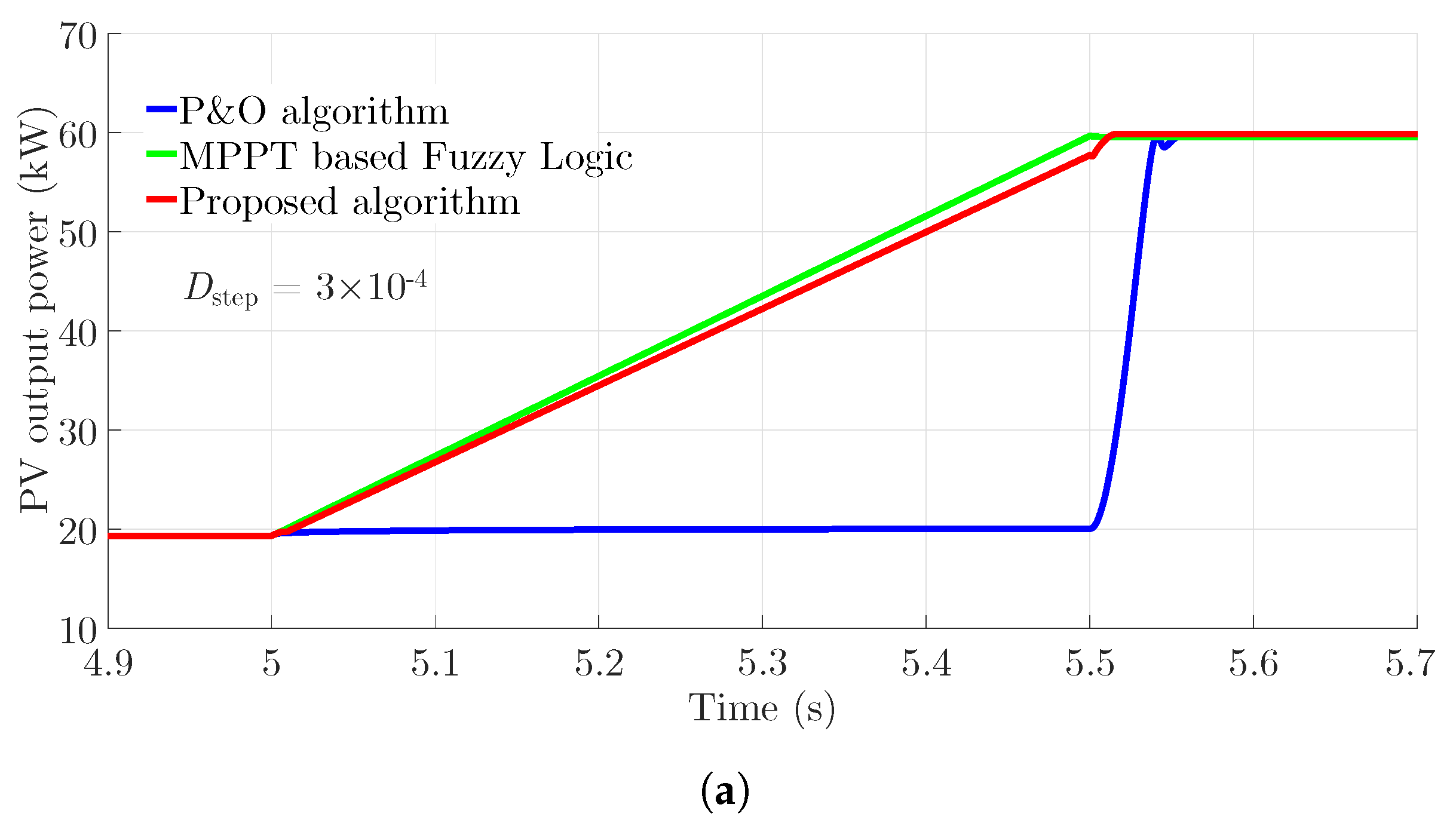
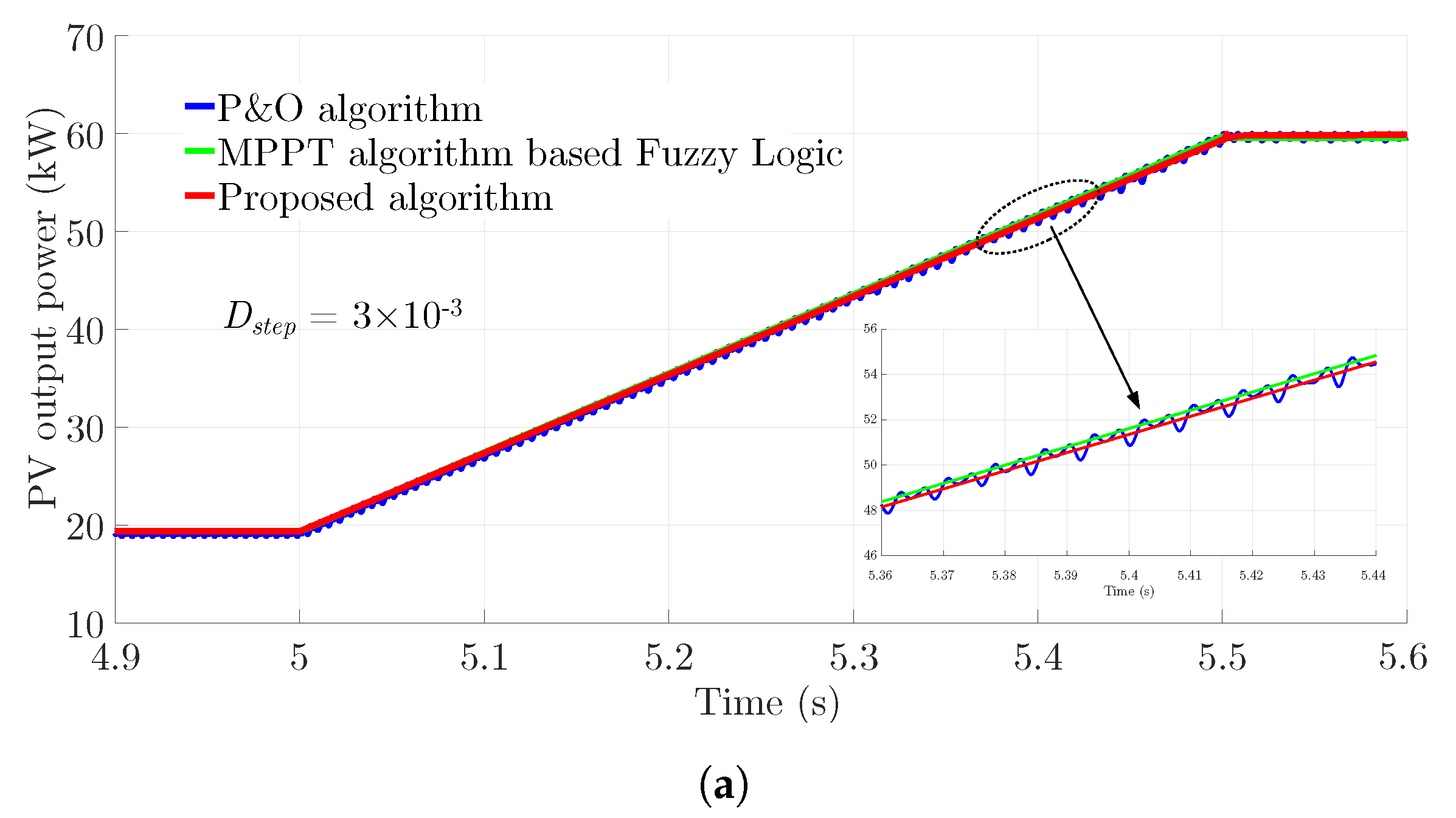
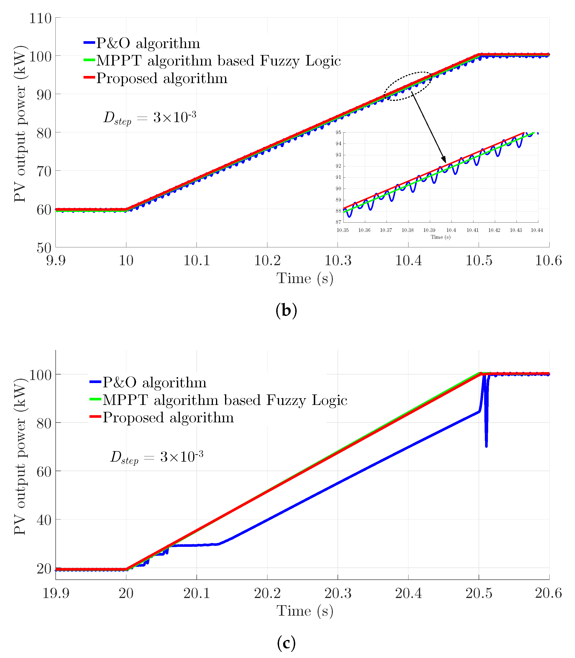
4.1. Rapid Increase of Solar Radiance

Figure 16 and Figure 17 show the PV array’s output power under the given value of panel temperature ($T=25$ ${}^{\circ }$C) and the rapid increase of solar radiance from 200 W/m${}^2$ to 600 W/m${}^2$, from 600 W/m${}^2$ to 1000 W/m${}^2$, and from 200 W/m${}^2$ to 1000 W/m${}^2$ within 0.5 s periods (Case 1 and Case 2). Figure 16 shows the simulation results with respect to $D_{step}=3\times {10}^{-4}$, and Figure 17 presents the results in the case of $D_{step}=3\times {10}^{-3}$.

Under these ambient conditions, the MPPT algorithm based on FL and the proposed algorithm are significantly more effective than the P&O method. As can be seen in Figure 16 and Figure 17, they respond to the radiance change almost instantaneously when the output power increases linearly along with the increase in radiance in all four cases. In contrast, the P&O algorithm shows a very poor tracking performance by witnessing an appreciable deviation from the MPP. Although it presents almost the same performance as the others when the duty cycle step $D_{step}$ is increased tenfold (from $3\times {10}^{-4}$ to $3\times {10}^{-3}$) in Case 1, it still cannot track the MPP properly in Case 2 with this increment of the duty cycle. Furthermore, in terms of output power oscillation, the proposed method and intelligent FL both present the least oscillation around the MPP.

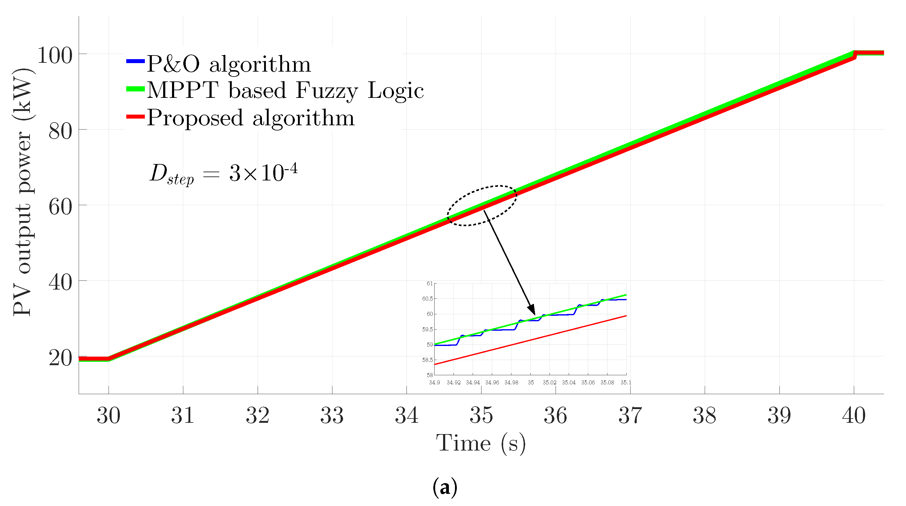
4.2. Slow Increase of Solar Radiance

In this case, a slow increase in solar radiance from 200 W/m${}^2$ to 1000 W/m${}^2$ within a time period of 10 s was simulated. As illustrated in Figure 18, the three MPPT techniques performed almost the same with two different values of $D_{step}$.

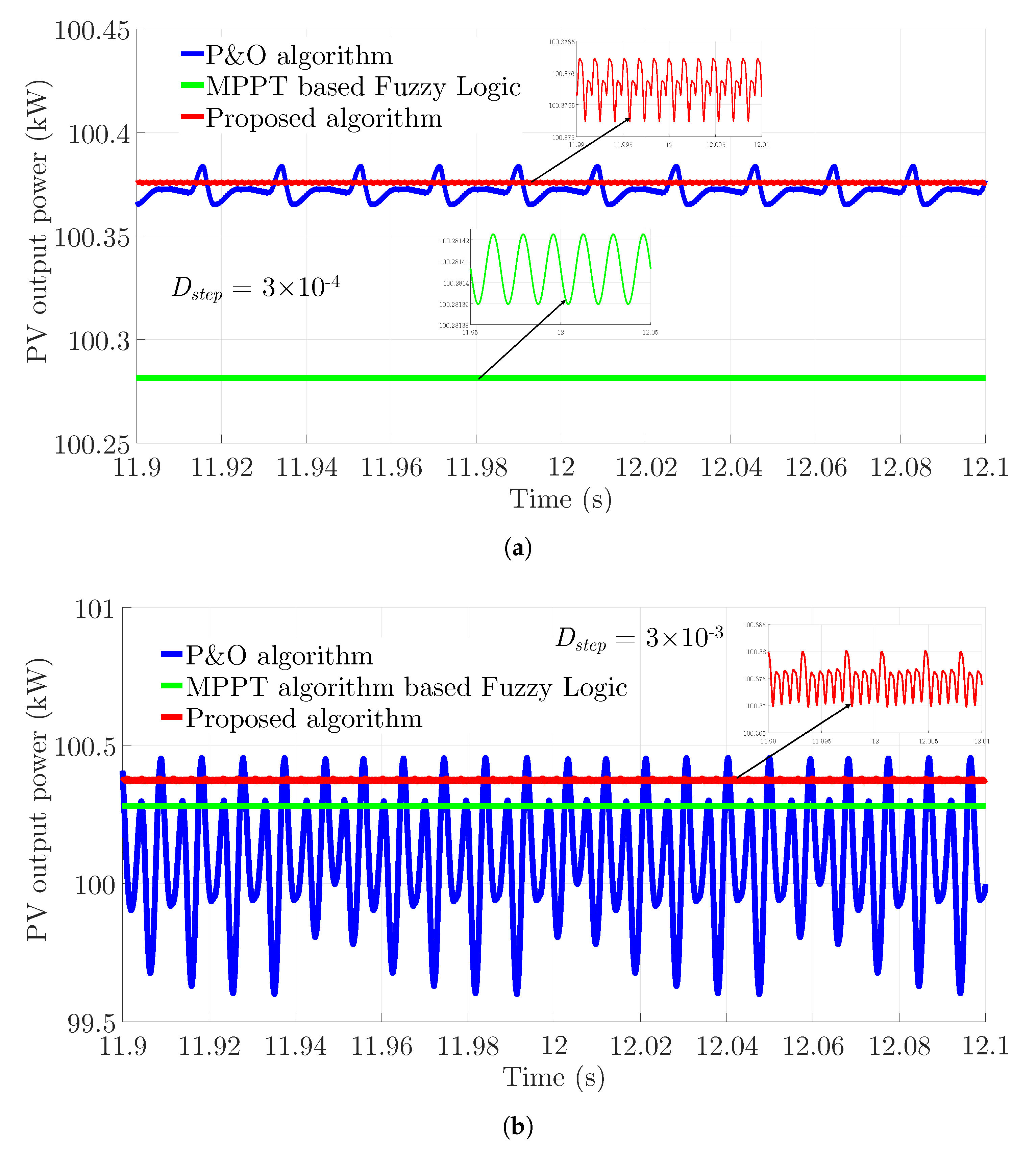
4.3. Stable Solar Radiance Condition

In this case, the radiance was kept constant at 1000 W/m${}^2$. The simulation results are illustrated in Figure 19. The P&O algorithm presented extremely significantly large power oscillation around the MPP in the steady state in comparison with the MPPT algorithms based on FL and the proposed algorithm, especially when the controller utilized $D_{step}=3\times {10}^{-3}$ to improve the MPP tracking speed. The P&O power oscillation level increased from about 18.8 W with $D_{step}=3\times {10}^{-4}$ to about nearly 854 W with $D_{step}=3\times {10}^{-3}$. When utilizing the proposed algorithm and the MPPT algorithm based on FL, the output power fluctuation was hardly noticed, just about 10 W and 0.3 W, respectively. An important thing that should be noted is that the proposed algorithm achieved more output power than the others. The detailed results of Figure 19 are shown in

Table 3. Average output power and oscillation power around the MPP under stable radiance at 1000 W/m${}^2$.

Algorithm	Average Output Power	Oscillation Level	Duty Cycle Step (${\mathit{D}}_{\mathit{step}}$)
P&O algorithm	100.37 kW	18.8 W	$3\times {10}^{-4}$
	100.1 kW	854 W	$3\times {10}^{-3}$
MPPT algorithm based on FL	100.28 kW	0.3 W
Proposed algorithm	100.38 kW	1 W	$3\times {10}^{-4}$
	100.37 kW	10 W	$3\times {10}^{-3}$

.

In terms of the proposed MPPT algorithm, we can see that it overcame the disadvantages of the traditional MPPT algorithms by satisfying the two requirements of an MPPT algorithm, which is fast convergence speed and small fluctuation of the output power. As shown in Table 3, in both cases of $D_{step}=3\times {10}^{-4}$ (small value) and $D_{step}=3\times {10}^{-3}$ (large value), the PV system using the proposed algorithm always tracked the MPP even when the solar radiation rapidly changed and the power fluctuation was very small, 1 W with $D_{step}=3\times {10}^{-4}$ and 10 W with $D_{step}=3\times {10}^{-3}$.

Generally, the tracking performances during the changing period of the solar radiance of different MPPT techniques are evaluated via the tracking efficiency ${\eta }_{MPPT}$, which is defined as [35,36]:

$${\eta }_{MPPT}={\displaystyle \frac{\underset{t_1}{\overset{t_2}{\int }}P\left(t\right)dt}{\underset{t_1}{\overset{t_2}{\int }}{P}_{\max }\left(t\right)dt}},$$

(4)

where $t_1$ and $t_2$ are the beginning and the end moments of the changing period, respectively, $P\left(t\right)$ is the actual PV output power, and $P_{\max }\left(t\right)$ is the theoretical maximum output power of the PV system. The efficiency obtained from Figure 16 to Figure 19 is shown in

Table 4. Comparison of the tracking efficiency for different MPPT techniques under various changing conditions of radiance.

Radiance Conditions	MPPT Efficient (${\mathit{\eta }}_{\mathit{MPPT}}$ %)
	P&O with ${\mathit{D}}_{\mathit{step}}=\mathbf{3}\times {\mathbf{10}}^{-\mathbf{4}}$	MPPT Based on FL	Proposed Algorithm with ${\mathit{D}}_{\mathbf{step}}=\mathbf{3}\times {\mathbf{10}}^{-\mathbf{4}}$
Rapid increase from $200\mathrm{W}/{\mathrm{m}}^2$ to $600\mathrm{W}/{\mathrm{m}}^2$	50.39	99.74	96.91
Rapid increase from $600\mathrm{W}/{\mathrm{m}}^2$ to $1000\mathrm{W}/{\mathrm{m}}^2$	75.13	99.46	99.77
Rapid increase from $200\mathrm{W}/{\mathrm{m}}^2$ to $1000\mathrm{W}/{\mathrm{m}}^2$	33.98	99.50	99.51
Stable condition	99.68	99.59	99.58
Radiance Conditions	MPPT Efficient(${\mathit{\eta }}_{\mathit{MPPT}}$ %)
	P&O with$D_{step}=3\times {10}^{-3}$	MPPT Based FL	Proposed Algorithm with$D_{step}=3\times {10}^{-3}$
Rapid increase from $200\mathrm{W}/{\mathrm{m}}^2$ to $600\mathrm{W}/{\mathrm{m}}^2$	99.19	99.74	99.34
Rapid increase from $600\mathrm{W}/{\mathrm{m}}^2$ to $1000\mathrm{W}/{\mathrm{m}}^2$	99.31	99.46	99.80
Rapid increase from $200\mathrm{W}/{\mathrm{m}}^2$ to $1000\mathrm{W}/{\mathrm{m}}^2$	81.79	99.50	99.15
Stable condition	99.40	99.59	99.70

.

The data shown in Table 4 indicate that the proposed MPPT algorithm tracks the MPP correctly under all considered cases of rapid changes of solar radiance and the tracking efficiencies are above 99% under most cases.

5. Conclusions

In this research, a new MPPT method based on the parameters of power variation ($\Delta P_{PV}$), voltage difference ($\Delta V_{PV}$), and the change of duty cycle ($\Delta D$) is proposed. The effectiveness of the proposed MPPT algorithm is verified by simulations in stable radiation conditions and in rapidly changing conditions. The simulated results show the fast convergence speed to the MPP of the PV system in the steady state and various weather conditions. In addition, fluctuations in the output power of the PV system are very small under stable radiation conditions, and there is no sudden capacity change in the case of rapidly changing weather conditions. Moreover, the proposed MPPT algorithm resolves the disadvantages of the traditional algorithms and has similar results as the MPPT algorithms using fuzzy intelligent control techniques. Finally, the proposed method shows the advantage of simple control rules, the efficiency enhancement of the PV system, low investment cost, and thus, the ease of application to all PV systems in an MG.

References

1. Liserre, M.; Sauter, T.; Hung, J.Y. Future Energy Systems: Integrating Renewable Energy Sources into the Smart Power Grid Through Industrial Electronics. IEEE Ind. Electron. Mag. 2010, 4, 18–37. [Google Scholar] [CrossRef]
2. Chaouachi, A.; Kamel, R.; Nagasaka, K. Microgrid efficiency enhancement based on neuro-fuzzy MPPT control for Photovoltaic generator. In Proceedings of the 2010 35th IEEE Photovoltaic Specialists Conference, Honolulu, HI, USA, 20–25 June 2010; pp. 2889–2894. [Google Scholar] [CrossRef]
3. Abdelsalam, A.; Massoud, A.; Ahmed, S.; Enjeti, P. High-Performance Adaptive Perturb and Observe MPPT Technique for Photovoltaic-Based Microgrids. Power Electron. IEEE Trans. 2011, 26, 1010–1021. [Google Scholar] [CrossRef]
4. Nguyen, V.T.; Hoang, D.H.; Nguyen, H.H.; Le, K.H.; Truong, T.K.; Le, Q.C. Analysis of Uncertainties for the Operation and Stability of an Islanded Microgrid. In Proceedings of the 2019 International Conference on System Science and Engineering (ICSSE), Dong Hoi, Vietnam, 20–21 July 2019; pp. 178–183. [Google Scholar]
5. Lam, L.; Phuc, T.; Hieu, N. Simulation Models For Three-Phase Grid Connected PV Inverters Enabling Current Limitation Under Unbalanced Faults. Eng. Technol. Appl. Sci. Res. 2020, 10, 5396–5401. [Google Scholar]
6. Park, H.; Kim, H. PV cell modeling on single-diode equivalent circuit. In Proceedings of the IECON 2013—39th Annual Conference of the IEEE Industrial Electronics Society, Vienna, Austria, 10–13 November 2013; pp. 1845–1849. [Google Scholar] [CrossRef]
7. Alrahim Shannan, N.M.A.; Yahaya, N.Z.; Singh, B. Single-diode model and two-diode model of PV modules: A comparison. In Proceedings of the 2013 IEEE International Conference on Control System, Computing and Engineering, Mindeb, Malaysia, 29 November–1 December 2013; pp. 210–214. [Google Scholar] [CrossRef]
8. Soon, J.J.; Low, K. Optimizing Photovoltaic Model for Different Cell Technologies Using a Generalized Multidimension Diode Model. IEEE Trans. Ind. Electron. 2015, 62, 6371–6380. [Google Scholar] [CrossRef]
9. Pandey, P.K.; Sandhu, K.S. Multi diode modelling of PV cell. In Proceedings of the 2014 IEEE 6th India International Conference on Power Electronics (IICPE), Kurukshetra, India, 8–10 December 2014; pp. 1–4. [Google Scholar] [CrossRef]
10. Babu, B.C.; Gurjar, S. A Novel Simplified Two-Diode Model of Photovoltaic (PV) Module. IEEE J. Photovolt. 2014, 4, 1156–1161. [Google Scholar] [CrossRef]
11. Mehta, H.K.; Warke, H.; Kukadiya, K.; Panchal, A.K. Accurate Expressions for Single-Diode-Model Solar Cell Parameterization. IEEE J. Photovolt. 2019, 9, 803–810. [Google Scholar] [CrossRef]
12. Shongwe, S.; Hanif, M. Comparative Analysis of Different Single-Diode PV Modeling Methods. IEEE J. Photovolt. 2015, 5, 938–946. [Google Scholar] [CrossRef]
13. Batushansky, Z.; Kuperman, A. Thevenin-based approach to PV arrays maximum power prediction. In Proceedings of the 2010 IEEE 26-th Convention of Electrical and Electronics Engineers in Israel, Eliat, Israel, 17–20 November 2010; pp. 598–602. [Google Scholar] [CrossRef]
14. Batzelis, E.I.; Kampitsis, G.E.; Papathanassiou, S.A.; Manias, S.N. Direct MPP Calculation in Terms of the Single-Diode PV Model Parameters. IEEE Trans. Energy Convers. 2015, 30, 226–236. [Google Scholar] [CrossRef]
15. Zagrouba, M.; Sellami, A.; Bouaicha, M.; Ksouri, M. Identification of PV solar cells and modules parameters using the genetic algorithms: Application to maximum power extraction. Sol. Energy 2010, 84, 860–866. [Google Scholar] [CrossRef]
16. Islam, M.N.; Rahman, M.Z.; Mominuzzaman, S.M. The effect of irradiation on different parameters of monocrystalline photovoltaic solar cell. In Proceedings of the 2014 3rd International Conference on the Developments in Renewable Energy Technology (ICDRET), Dhaka, Bangladesh, 29–31 May 2014; pp. 1–6. [Google Scholar]
17. Razak, A.; Yusoff, M.; Leow, W.Z.; Irwanto, M.; Ibrahim, S.; Zhafarina, M. Investigation of the Effect Temperature on Photovoltaic (PV) Panel Output Performance. Int. J. Adv. Sci. Eng. Inf. Technol. 2016, 6, 682. [Google Scholar] [CrossRef]
18. Santos, J.; Antunes, F.; Chehab, A.; Cruz, C. A maximum power point tracker for PV systems using a high performance boost converter. Sol. Energy 2006, 80, 772–778. [Google Scholar] [CrossRef]
19. Kebir, G.; Larbes, C.; Ilinca, A.; Obeidi, T.; Kebir, S. Study of the Intelligent Behavior of a Maximum Photovoltaic Energy Tracking Fuzzy Controller. Energies 2018, 11, 3263. [Google Scholar] [CrossRef] [Green Version]
20. Subudhi, B.; Pradhan, R. A Comparative Study on Maximum Power Point Tracking Techniques for Photovoltaic Power Systems. IEEE Trans. Sustain. Energy 2013, 4, 89–98. [Google Scholar] [CrossRef]
21. Nguyen, B.N.; Nguyen, V.T.; Duong, M.Q.; Le, K.H.; Nguyen, H.H.; Doan, A.T. Propose a MPPT Algorithm Based on Thevenin Equivalent Circuit for Improving Photovoltaic System Operation. Front. Energy Res. 2020, 8, 14. [Google Scholar] [CrossRef] [Green Version]
22. Esram, T.; Chapman, P.L. Comparison of Photovoltaic Array Maximum Power Point Tracking Techniques. IEEE Trans. Energy Convers. 2007, 22, 439–449. [Google Scholar] [CrossRef] [Green Version]
23. Bendib, B.; Belmili, H.; Krim, F. A survey of the most used MPPT methods: Conventional and advanced algorithms applied for photovoltaic systems. Renew. Sustain. Energy Rev. 2015, 45, 637–648. [Google Scholar] [CrossRef]
24. Hohm, D.; Ropp, M. Comparative Study of Maximum Power Point Tracking Algorithms. Prog. Photovolt. Res. Appl. 2003, 11, 47–62. [Google Scholar] [CrossRef]
25. Femia, N.; Petrone, G.; Spagnuolo, G.; Vitelli, M. Optimization of Perturb and Observe Maximum Power Point Tracking Method. Power Electron. IEEE Trans. 2005, 20, 963–973. [Google Scholar] [CrossRef]
26. Kollimalla, S.K.; Mishra, M.K. A Novel Adaptive P O MPPT Algorithm Considering Sudden Changes in the Irradiance. IEEE Trans. Energy Convers. 2014, 29, 602–610. [Google Scholar] [CrossRef]
27. Piegari, L.; Rizzo, R. Adaptive perturb and observe algorithm for photovoltaic maximum power point tracking. IET Renew. Power Gener. 2010, 4, 317–328. [Google Scholar] [CrossRef]
28. Tan, C.W.; Green, T.C.; Hernandez-Aramburo, C.A. An Improved Maximum Power Point Tracking Algorithm with Current-Mode Control for Photovoltaic Applications. In Proceedings of the 2005 International Conference on Power Electronics and Drives Systems, Kuala Lumpur, Malaysia, 28 November–1 December 2005; Volume 1, pp. 489–494. [Google Scholar] [CrossRef]
29. Algazar, M.; AL-monier, H.; EL-halim, H.; Salem, M. Maximum power point tracking using fuzzy logic control. Int. J. Electr. Power Energy Syst. 2012, 39, 21–28. [Google Scholar] [CrossRef]
30. Saleh, A.; Faiqotul Azmi, K.S.; Hardianto, T.; Hadi, W. Comparison of MPPT Fuzzy Logic Controller Based on Perturb and Observe (P&O) and Incremental Conductance (InC) Algorithm On Buck-Boost Converter. In Proceedings of the 2018 2nd International Conference on Electrical Engineering and Informatics (ICon EEI), Batam, Indonesia, 16–17 October 2018; pp. 154–158. [Google Scholar] [CrossRef]
31. Patcharaprakiti, N.; Premrudeepreechacharn, S. Maximum power point tracking using adaptive fuzzy logic control for grid-connected photovoltaic system. In Proceedings of the 2002 IEEE Power Engineering Society Winter Meeting, Conference Proceedings (Cat. No.02CH37309), New York, NY, USA, 27–31 January 2002; Volume 1, pp. 372–377. [Google Scholar] [CrossRef]
32. Bendib, B.; Krim, F.; Belmili, H.; Almi, M.F.; Bolouma, S. An intelligent MPPT approach based on neural-network voltage estimator and fuzzy controller, applied to a stand-alone PV system. In Proceedings of the 2014 IEEE 23rd International Symposium on Industrial Electronics (ISIE), Istanbul, Turkey, 1–4 June 2014; pp. 404–409. [Google Scholar] [CrossRef]
33. Chekired, F.; Mellit, A.; Kalogirou, S.; Larbes, C. Intelligent maximum power point trackers for photovoltaic applications using FPGA chip: A comparative study. Sol. Energy 2014, 101, 83–99. [Google Scholar] [CrossRef]
34. Shiau, J.K.; Wei, Y.C.; Chen, B.C. A Study on the Fuzzy-Logic-Based Solar Power MPPT Algorithms Using Different Fuzzy Input Variables. Algorithms 2015, 8, 100–127. [Google Scholar] [CrossRef] [Green Version]
35. Hua, C.; Shen, C. Study of maximum power tracking techniques and control of DC/DC converters for photovoltaic power system. In Proceedings of the PESC 98 Record, 29th Annual IEEE Power Electronics Specialists Conference (Cat. No.98CH36196), Fukuoka, Japan, 22–22 May 1998; Volume 1, pp. 86–93. [Google Scholar] [CrossRef]
36. Pei, T.; Hao, X.; Gu, Q. A Novel Global Maximum Power Point Tracking Strategy Based on Modified Flower Pollination Algorithm for Photovoltaic Systems under Non-Uniform Irradiation and Temperature Conditions. Energies 2018, 11, 2708. [Google Scholar] [CrossRef] [Green Version]
Figure 1. Single-diode model of a PV cell.
Energies 13 04326 g001
Figure 2. Typical current–voltage curve for a PV array.
Energies 13 04326 g002
Figure 3. Structure of a typical MPPT.
Energies 13 04326 g003
Figure 4. Perturb and observe algorithm’s flowchart.
Energies 13 04326 g004
Figure 5. Path of the PV array’s operating point with the P&O algorithm under slowly and rapidly changing radiation (Adapted from [23]).
Energies 13 04326 g005
Figure 6. The hill-shaped curve of the P P V D characteristic of the MPPT boost converter.
Energies 13 04326 g006
Figure 7. Hill climbing algorithm’s flowchart.
Energies 13 04326 g007
Figure 8. Basic structure of the FL controller.
Energies 13 04326 g008
Figure 9. (a) Membership function input variable Δ V P V ; (b) Membership function input variable Δ P P V . NB, Negative Big; NM, Negative Moderate; NS, Negative Small; ZE, Zero; PS, Positive Small; PM, Positive Moderate; PB, Positive Big.
Energies 13 04326 g009
Figure 10. (a) Fuzzy regions for P P V V P V curve; (b) Fuzzy rules for algorithm using Δ V P V and Δ P P V as the inputs.
Energies 13 04326 g010
Figure 11. Membership functions for output variable Δ D .
Energies 13 04326 g011
Figure 12. Proposed MPPT algorithm.
Energies 13 04326 g012
Figure 13. Responses of the proposed algorithm when solar radiation is unchanged: Path 1 or Path 2.
Energies 13 04326 g013
Figure 14. Responses of the proposed algorithm when solar radiation is stable: Path 3, Path 4, or Path 5.
Energies 13 04326 g014
Figure 15. Waveform of solar radiance.
Energies 13 04326 g015
Figure 16. Comparison of the output power in the case of solar radiance increasing rapidly within 0.5 s periods and with D s t e p = 3 × 10 4 : (a) solar radiance increase from 200 W/m2 to 600 W/m2; (b) solar radiance increase from 600 W/m2 to 1000 W/m2; (c) solar radiance increase from 200 W/m2 to 1000 W/m2 .
Energies 13 04326 g016aEnergies 13 04326 g016b
Figure 17. Comparison of the output power in the case of solar radiance increasing rapidly within 0.5 s periods and with D s t e p = 3 × 10 3 : (a) solar radiance increase from 200 W/m2 to 600 W/m2; (b) solar radiance increase from 600 W/m2 to 1000 W/m2; (c) solar radiance increase from 200 W/m2 to 1000 W/m2
Energies 13 04326 g017aEnergies 13 04326 g017b
Figure 18. Comparison of the output power in the case of solar radiance increasing slowly from 200 W/m 2 to 1000 W/m 2 within 10 s: (a) D s t e p = 3 × 10 4 ; (b) D s t e p = 3 × 10 3 .
Energies 13 04326 g018aEnergies 13 04326 g018b
Figure 19. Comparison of the output power in the case of solar radiance being stable at 1000 W/m 2 : (a) D s t e p = 3 × 10 4 ; (b) D s t e p = 3 × 10 3 .
Energies 13 04326 g019