Abstract
This article presents a comparative experimental evaluation of some power calculation methods used for three-phase and single-phase systems. In order to make the comparison, methods based on three reference frames, the natural one, αβ and dq, are considered. This paper addresses the experimental comparison for single-phase systems facing sinusoidal and non-sinusoidal waveforms in both linear and non-linear loads. The results are obtained from an experimental platform consisting of a controlled voltage inverter and an acquisition system based on a TMS320F28335, where the power calculation algorithms are implemented. The experimental comparison of the different methods for active and reactive power calculation is made in terms of accuracy and processing time in digital implementation.
1. Introduction
Electrical systems have been immersed in constant technological challenges due to the introduction of renewable energy generators, storage systems, the bidirectionality of energy, distributed generation and electrical microgrids [1,2,3]. For these electrical systems, it is necessary to transmit, distribute, monitor, control, commercialize and exchange power [4], among other functions [5], and, therefore, its measurement and calculation are relevant. Nowadays, the incursion of electronic equipment, electronic converters [6] and the use of non-linear loads have caused a constant increase in harmonic distortion in power systems [7], which must be quantified in power from its precise measurement and there are several disturbances that could cause excessive errors in digital input electricity meters, for example, the influence caused by frequency offset [8], distorted signals and/or unbalanced sequences with different levels for fundamental frequency deviation, waveform distortion, harmonic frequencies, voltage unbalance, zero sequence, and so on [9].
In the presence of non-sinusoidal voltage and current signals, different definitions for power calculation have been proposed in the literature. Thus, different types of power definitions can be found in the IEEE 100-88 standard dictionary of electrical and electronic terms as well as discussions for such definitions [10]. In the IEEE Std.1459-2010 there are definitions for the measurement of power quantities under sinusoidal, non-sinusoidal, balanced and unbalanced conditions. In [11], a review of several definitions is presented such as those proposed by Budeanu [12], Fryze [13], Shepherd-Zakikhani, Sharon, Depenbrock, Kusters-Moore, and Czarnecki [14], mainly to validate which of these are appropriate for power factor maximization. Several of them have been formulated based on the decomposition of the power triangle, such as the Budeanu definition, applied only in the analysis of stable state and therefore limited to periodic voltage and current waveforms. Consequently, the voltage and current signals can be decomposed in Fourier series [15]. Other approaches can be found for the calculation of the instantaneous power based on Hilbert’s Transform, which allows one to define the instantaneous active and reactive power in single-phase circuits operating in the transient state for single-phase systems [16]. Some methodologies are presented in the literature for quality assurance of energy meters; in [9], a methodology based on a design of experiment to guide verification of energy meters under sinusoidal and non-sinusoidal conditions was presented; in [8], a triangular window weighted algorithm is proposed for reducing the influence of frequency offset remarkably and guarantee good real-time performance at the same time.
When calculating the power in a system, just as it is done in measuring equipment, it is necessary to calculate the power in programmable electronic devices to perform calculations of apparent, active, reactive power and power factor. Various applications require this calculation; for example, for the exchange of power with the electrical grid [4], it is necessary to calculate the active and reactive power from the measurement of current and voltage to control the distribution of power in electric microgrids using the droop control technique [17]. In [9], a power calculation method is proposed for the improved UPS system that shows better current-sharing performance, taking the inductor current instead of the output current.
This is also applied for decisions in economic engineering [5]. In the case of three-phase systems, it is easy to calculate the active and reactive power from the dq transformation. In the synchronous reference frame, this transformation allows for performing simple mathematical operations for the calculation of powers with live and quadrature values. For single-phase systems, it is required to generate a signal delayed 90° respect to the measured voltage signal. This 90° phase shift operation has been proposed by different methods, such as the quarter-cycle time delay of the fundamental frequency [18], diverter [8,19], integrator [19], low-pass filter, all-pass filter [19], Hilbert transform, second-order generalized integrator (SOGI) [20] or by Enhanced Phase-locked Loop (EPLL) [21], among others [4]. In this paper, some of these techniques are compared in the natural reference frame, as well as the mathematical operations techniques in the αβ and dq reference frame.
2. Materials and Methods
As mentioned above, there are several methods to calculate the active and non-active power. All these require as input the current and voltage functions in the time domain. In addition, for the application of several of these methods in the measurement of power in single-phase systems, the generation of signals that simulate voltages and dummy currents from real measurements is required. Thus, for the real-time digital implementation of these power calculation methods, rapid sampling and processing systems are required.
To make the comparison of the methods of calculation of electrical power, in this work, an experimental platform is used that is composed of a controlled voltage source that feeds different types of load and a digital acquisition and processing system for the implementation of the calculation methods of active and non-active power.
The experimental platform is represented in Figure 1, the controlled source is obtained from a voltage inverter with an LC filter, while a TMS320F28335 DSC is used to perform the power calculations, which converts to digital the voltage and current measurements on the load, generates the additional signals required by the power calculation methods, performs the operations of the respective method and calculates the average value generated by the power calculation methods.
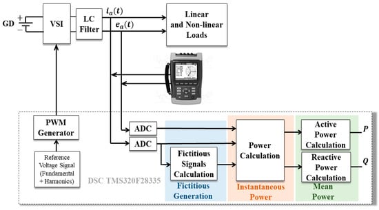
Figure 1.
Power measurement system.
Thus, before conducting the experimental comparison between the different methods considered, the rest of this section describes these methods in a conceptual way. These methods are here classified according to the reference framework. Hence, the methods considered for the natural framework are time delay, time delay integrator, all-pass filter, state observer, Hilbert transform and mathematical operations. Similarly, the calculation is considered directly on the stationary reference frame αβ0 and on the rotating frame dq0.
2.1. Natural Frame Methods for Single-Phase Systems
The methods for the generation of the orthogonal signal are used in the natural frame “abc”. The phase “a” is the one already having the single-phase system, being either the voltage or the current signal. Therefore, phase “b” is generated from phase “a” by using methods that may generate either an orthogonal or a quadrature signal such as the following ones.
2.1.1. Time Delay Method
As shown in Figure 2, for reactive power calculation q, this method seeks to obtain a time delay of a quarter of a cycle of the fundamental component (T/4) with the aim of generating a 90° lagged signal with respect to the signal of a single-phase generator.
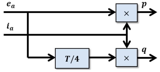
Figure 2.
Power calculation with Time delay method.
One of the most important considerations to bear in mind using this method is when the signal has harmonic components of order h, these will not have a 90° delay but of h times 90° instead, something that could generate errors in the final signal [22]. In general, this quarter-cycle delay method has a fundamental characteristic: it only works well with signals completely free of harmonic components; otherwise, the output signal presents considerable and inadmissible distortions for the possible calculation of power.
2.1.2. Time Delay Integrator Method
This method relies on the use of an integrator to obtain a 90° phase lag for every frequency component of the input signal (see Figure 3), a unitary gain for the fundamental component, as is shown in (1), with amplitude and frequency . Since its magnitude response is inversely proportional to the frequency of the input signal, it also changes the amplitude of the harmonic components [22].
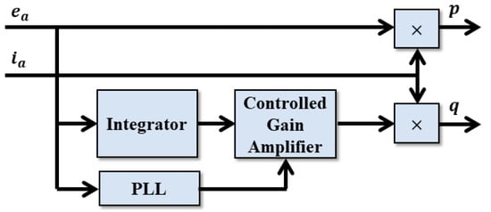
Figure 3.
Power calculation by integration method.
This implies that a strategy must be implemented to recover the signal amplitude at the integrator output. It is possible to implement a programmable-gain amplifier, which could perform the compensation in an adaptive way depending on the frequency, for this reason, it is also necessary a frequency meter like a PLL (Phase Locked Loop) [22]. However, the system is very sensitive to the change of amplitude by any small variation that the integrator may generate. It is also necessary to implement a high-pass filter at the output to block the DC levels that may occur. In general, this method presents a difficult problem to deal with, which is the heavy dependence of the amplitude in the output signal with respect to the input frequency. In addition, the gain used after the integration block must be calculated with great precision to not only reach the desired amplitude but also in order not to alter the power measurement assuming that the input sinusoidal signal remains unchanged. Nonetheless, this is a situation that may not be easy to ensure in practice.
2.1.3. All-Pass Filter Method
The all-pass filter method implements a first-order filter, whose voltage transfer function has a unit gain and a phase that depends on the ω frequency at which the filter is designed [23]. The typical transfer function of the all-pass filter is shown in Equation (2), with = 2πf.
In this method, the magnitude of the output remains constant and does not present variations induced by the filter and the phase is exactly 90° to the work frequency (50 Hz and 60 Hz). However, the filter also shifts the phase of other frequency components by a different amount.
2.1.4. State Observer Method
Another way to generate the orthogonal signal is by using a Luenberger observer. The power calculation by state observer method is shown in the Figure 4.
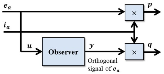
Figure 4.
Power calculation by state observer method.
The observer design proposed follows the idea in [24], which starts from a single-phase sinusoidal oscillator as shown in Figure 5. The desired steady-state solution from the oscillator is given by and , where is the frequency of oscillator in rad/sec and x1, x2 are the state variables.
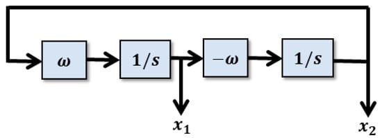
Figure 5.
Single-phase sinusoidal Oscillator.
The state variable of the oscillator Equation (3) is modified as a state observer, as shown Equation (4) by adding the Luenberger observer feedback constants and to be evaluated.
where is the original signal (the one to be measured), is the fictitious signal that is orthogonal to and is the fundamental frequency of Moreover, and are constants that are calculated from the characteristic equation of the state observer (5) [25].
In [25], the poles of the state observer are selected as s1 = s2 = −10ω and the same criterion will be used. Thus, after clearing the characteristic equation for , the following constant values are obtained in (6):
Replacing (6) in (4), we have (7):
2.1.5. Hilbert Transform Method
The Hilbert’s Transform method is also used to generate orthogonal signals. This method is based on the application of the Hilbert transform, and ideally, such transformation is linear and generates a unit gain. In addition, the phase shift is +90° for all negative frequencies and −90° for all positive frequencies [22]. The function with which these method works is shown in (8):
The disadvantage of this method lies in its practical elaboration since the implementation of high-order filters is required in order to have an approximation to the ideal response.
2.1.6. Method Using Mathematical Operations
This method, proposed in [26], uses orthogonal signal generators for voltage and current. The method seeks to avoid the use of a low-pass filter so that the calculation of active and reactive power is faster when the droop control of active and reactive power distribution is performed in microgrids. In this method, the authors propose a novel way of calculating the active and reactive power in an easy way and with a high system response time. The use of the low-pass filter needed for power measurement in conventional methods in the abc reference frame is eliminated and the process is performed using only 90° phase shifts, multiplications, and additions. Figure 6 [26], shows the original schemes proposed for the active and reactive power calculation.
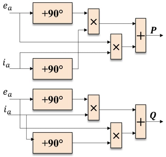
Figure 6.
Power calculation by Math Operations with a filter. Active power calculation (top). Reactive Power calculation (down).
2.2. Power Calculation in the αβ0 Stationary Reference Frame
Another method for calculating the active and reactive power can be carried out from the stationary reference frame employing the power invariant Clarke transformation, commonly known as method αβ0 [15]. As shown in Figure 7, it is necessary that the transformation matrices from the natural reference frame to the reference frame αβ0 have all the inputs enabled. In other words, it is necessary that the voltage and current signals of the single-phase system are connected directly to the inputs “a” of the reference frame converter blocks. Additionally, it is also essential that the other inputs, “b” and “c”, respectively, have the same inputs but with a phase shift of 120° for the former and 240° for the latter.
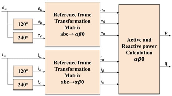
Figure 7.
Power calculation by αβ0 method.
The reference frame transformation matrices are shown in Equation (9). The respective active and reactive power calculation is shown in Equations (10) and (11).
2.3. Power Calculation in the dq0 Rotating Reference Frame
The calculation of active and reactive power in a single-phase system under the rotating reference frame has the advantage of delivering an almost constant value of active and reactive power as it is a rotating reference frame, commonly called the dq0 method [6]. As shown in Figure 8, an additional element is required to constantly calculate the rotation angle, such as a PLL. Since a single-phase system is used, the sample signals are taken and connected to the input “α” of the transformation blocks from the reference frame αβ0 to the reference frame dq0, in order to carry out the measurement correctly. At the same time, the original sample signals are taken, and a 90° delay is applied to them and then connected to the “β” inputs of the same transformation modules. The idea is to take the signals in the abc reference frame but as if they were working in the αβ0 reference frame with a 90° phase difference between the signals.
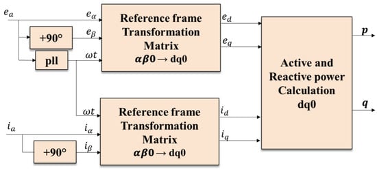
Figure 8.
Power calculation by dq0 method.
The transformation matrix from the reference frame αβ0 to the reference frame dq0 is shown in Equation (12) with θ = ωt.
The active and reactive power in this dq DQ reference frame is calculated as shown in (13) and (14), respectively.
For this measurement, the zero sequence is eliminated in the dq DQ reference frame for the single-phase system.
3. Experimental Results and Discussion
The experimental results of the applied calculation methods are obtained from voltage and current measurements for an RL load (linear) and uncontrolled bridge rectifier load (non-linear). These loads are fed separately from a DC source with a single-phase voltage source inverter. In the inverter its reference signal is adjusted to obtain different operating conditions. The Voltage Source Inverter (VSI) shown in the Figure 1 was implemented in a SEMITEACH B6U+E1CIF+B6CI provided by Semikron. The single-phase VSI topology is a full bridge with bipolar-SPWM modulation. For this purpose, it is considered VSI sinusoidal and non-sinusoidal output voltages from fundamental frequency f up to the seventh harmonic of the fundamental frequency, which was chosen as an operating frequency range from 60 to 420 Hz, respectively. To achieve this, a switching frequency of 10080 Hz was selected for both the IGBT’s commutation frequency limitation recommended by the manufacturer to be less than 20 kHz and a multiple of the fundamental frequency. The criterion for the selection of the LC filter parameters at the VSI output was to take a cut-off frequency, a one decade below of switching frequency fsw, for which 1 kHz was chosen. Additionally, to ease the digital control design and to reduce the delay of digital implementation [27], using TMS32028F335, a triangular carrier was used for achieving a sampling frequency fs of 20160 Hz. The LC filter has two functions to attenuate the output voltage ripple and to limit the high-frequency ripple current of VSI IGBTs [28]. On the other hand, the RL load was selected by the power capacity of the voltage supply in the DC bus and by the maximum current that the electronic sensor board handles at 2A. The non-linear load was designed by the IEC 62040-3 standard to obtain a crest factor of 2.9 [27]. Table 1 shows the inverter characteristics and the test loads values.

Table 1.
Electrical features of the inverter and test loads.
Experimental data are obtained from an LTS 6-NP LEM current sensor and an LV 25-P LEM voltage sensor connected directly to the test load. The output signals are conditioned and carried to two ADC inputs collected from the TMS320F28335. Subsequently, these signals are processed through the CCS software (Code Composer Studio), in which three cycles of the active and reactive power signals of each programmed method in C language are acquired. The data in CCS® are exported and processed in MATLAB. At the end of this section, the results of the calculation time used by the different methods in the DSC are shown.
3.1. Experimental Validation: Active and Reactive Power Calculation for an RL Load
To test the performance of the considered power calculation methods, an RL series test load (R = 64.2 Ω and L = 18.8 mH) is fed with a non-sinusoidal voltage waveform. Regarding this matter, the maximum limits of harmonic content in a sinusoidal signal described in the IEEE standard 519-2014 [29] were initially considered. However, the theoretical calculation for each of the power inputs of all the harmonic components proposed in this standard is somehow very cumbersome and long. For this reason, the VSI reference signal is synthesized by adding to the fundamental component, the 3rd, 5th and 7th harmonic components with an amplitude of 30% of the fundamental component. Such amplitudes were greater than those proposed in the standard so that the distortion would become more evident in all the methods to be tested without having to contain the harmonic components up to the 33rd order or higher.
Analytical calculations are performed according to the definitions present in the IEEE 1459-2010 standard [30]. As mentioned in the introduction of this section, Figure 9 shows the current and voltage waveforms obtained for the RL series load under 4 different operation conditions. Each one of those 4 waveform sets were obtained by setting the VSI voltage reference to synthesize waveforms with different harmonic content. The experiments performed are as follows: (1) Only the fundamental component, (2) fundamental and 3rd harmonic, (3) fundamental, 3rd and 5th harmonic, 4) fundamental, 3rd, 5th and 7th harmonic.
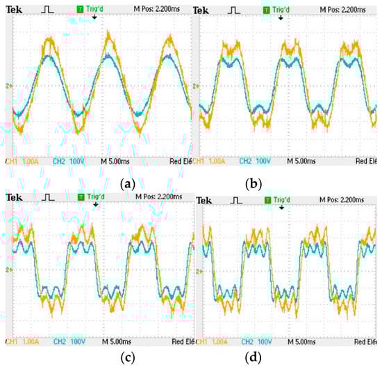
Figure 9.
Voltage (green) and current (orange) signals: (a) fundamental; (b) fundamental + 3rd harmonic; (c) fundamental + 3rd + 5th harmonic; (d) fundamental + 3rd + 5th + 7th harmonic.
The voltage and current signals in the RL load are obtained in a Tektronics TDS 2012C digital oscilloscope. The voltage differential probe, Tektronics P5200A, has a 500X attenuation range and the Fluke I400s probe is on the 10 mV/A scale. Besides the methods explained in Section 2, another two new methods are tested here. Those two methods are modifications of the αβ0 method and the mathematical operations method, they are here are referred to as Alpha-Beta with filter and Mathematical operations method with filter, respectively. Those modifications consist of digitally filtering the output signal of each of those methods.
Figure 10, shows the time response of the different power calculation methods considered in this comparison. As can be seen, in general terms, the speed response of the original mathematical operations method is the fastest to be established for both, active and reactive power, with less than one period of the fundamental signal. The original αβ method is the second fastest, with only one and a half cycles of the fundamental. On the other hand, the other methods take approximately 5.4 cycles of the fundamental to reach their steady-state value.
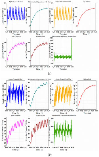
Figure 10.
Power time responses: (a) active power; (b) reactive power (down).
The active and reactive power measurements are taken with the Fluke 1730 instrument, which was chosen as a reference. The calculated error method is based on experimental measurements with Fluke 1730.
Figure 11 shows the experimental results of the calculation of active and reactive power at the RL load when the VSI does not have a harmonic component and the numeric results are shown in Table 2. The unfiltered mathematical operations and αβ methods present large oscillations of active and reactive power, which may not be adequate when precise measurements are required at certain periods of the fundamental signal. For example, in the case of active power sharing in droop-controlled inverters, these two methods will result in a frequency that is changing at the same time as the measured value of the active power changes the frequency will be changing.
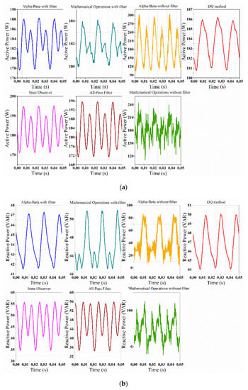
Figure 11.
Power calculation methods at the fundamental frequency: (a) active power; (b) reactive power.
Table 2.
Experimental results for RL load.
The method using mathematical operations, in its version with an averaging filter, presents less oscillation in a steady state with respect to the other methods. In the natural reference frame, this would be the best method to measure active and reactive power in ideal conditions of a sinusoidal input without harmonic content. However, the State Observer method presented the lowest active power error with 3.1302% and 14.267% for the reactive power, respectively, with respect to the Fluke 1730 measurement with an error of 4.3733%. On the other hand, the αβ method without a filter is the one that deviates the most in reactive power with 18.938%, as shown in Table 3.
Table 3.
Experimental results error %.
In the second experiment, the third harmonic component is added. In Figure 12, the oscillations of the mathematical operations and the αβ methods have increased. In addition, it is shown that there is a great deviation given by the αβ and the mathematical operations methods with filter, mainly for reactive power.
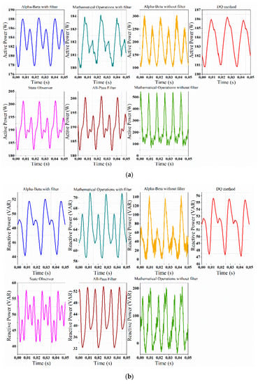
Figure 12.
Power calculation at fundamental frequency + 3rd harmonic: (a) active power; (b) reactive power.
The mathematical operations method exposes the highest percentages of error in active power: 17.766% when it does not have the filter and 18.072% when it does. The highest percentage of error for reactive power is presented by the all-pass filter method, with 51.657%. The DQ and State Observer methods retain good behavior in terms of the amplitude of oscillations and regularity of error in a steady state for both, active and reactive power. In the active power, the lowest error is shown by the αβ method, whereas the lowest error for the reactive power is given by the mathematical operations method with filter. Figure 13 shows the active and reactive power for the system with a third harmonic plus fifth harmonic component.
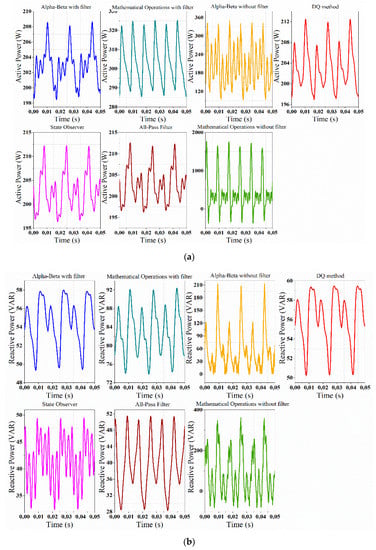
Figure 13.
Power calculation at fundamental frequency + 3rd harmonic + 5th harmonic: (a) active power; (b) reactive power.
In this Figure, it is still observed that the oscillations are increasing for the αβ and the mathematical operations methods. On the other hand, both the state observer, the αβ with and without filter, as well as the DQ methods result in a lower error of 6.64% for the active power. Now, for the reactive power, the methods of mathematical operations with and without the filter of 34.99% and 35%, respectively, have a lower stationary error.
In Figure 14, taking into account that the system presents harmonic content comprising the third, fifth and seventh harmonics, it is verified that the mathematical operations method presents high peaks of active and reactive power in a very short time as the number of harmonics increases, as shown in Table 2. In the same sense, the αβ method allows it but with less amplitude.
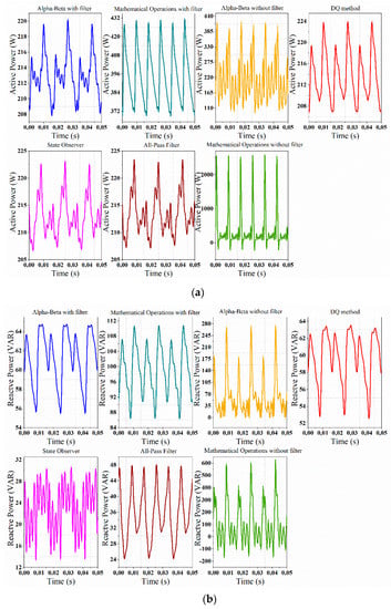
Figure 14.
Power calculation at fundamental frequency + 3rd harmonic + 5th harmonic + 7th harmonic: (a) active power; (b) reactive power.
For active power, as shown in Table 3, all methods have an error of less than 13%, except for the mathematical operations methods that present a very high error margin. On the contrary, for reactive power, the mathematical operations methods would be the most appropriate because they present a lower error margin. However, these errors are very high, as shown in Table 3.
3.2. Experimental Validation: Active and Reactive Power Calculation for a Non-Linear Load
The non-linear load consists of a full-wave rectifier with a 420-μF capacitor and a 136-Ω resistor, with a current crest factor of 2.9. Figure 15 shows the waveforms of voltage and current on the test load. Figure 16, shows the experimental results of the calculation of active power for the non-linear load.
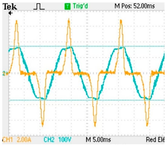
Figure 15.
Waveforms of the current and voltage in oscilloscope for the non-linear load.
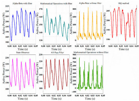
Figure 16.
Active power calculation with all methods at the fundamental frequency—non-linear load.
The graph on the left shows the results of all methods, whereas the graph on the right describes an enlargement of the result of only five of these methods with a better resolution to appreciate their behavior.
In the figure on the left, the amplitudes of ripples of the active power for the αβ and for the mathematical operations methods without a filter are the largest. However, despite this fact, such methods give the fastest response. It is worth mentioning that these two methods do not have a filter. On the other hand, an enlarged view of only five of these methods can be observed in the figure on the right, where two of these are the αβ and the mathematical operations methods, but with filter. In this zoom, it can be detailed that the answers are very similar in amplitude and response time among all the methods, being the method of mathematical operations with filter the one that deviates most in the stationary state, as is shown in Table 4.
Table 4.
Experimental measurements—non-linear load.
Figure 17, shows the experimental results of the reactive power for non-linear load. The graph on the left describes the result of all methods, whereas the enlarged graph on the right shows the results of only five methods without the original αβ and mathematical operations methods without a filter.
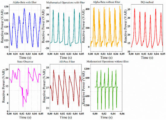
Figure 17.
Reactive power calculation with all methods at the fundamental frequency—non-linear load.
The αβ and the mathematical operations methods without filter, although they present large oscillations compared to the other ones, are equally imprecise to the other methods. However, methods αβ with and without filter, which present the closest stationary state value in reactive power with respect to the Fluke 1730 measurement, make an exception, as clearly shown in Table 5.
Table 5.
Error percentage for each method—non-linear load.
3.3. Calculation Time of Active and Reactive Power
The processing time used by the different active and reactive power calculation algorithms in the DSC TMS320F28335 is shown in Table 6.
Table 6.
Calculation times.
The results obtained in Table 6 show that the all-pass Filter, as well as the state observer methods, are the fastest, with 5.2 μs of runtime in the DSP. These are followed by the mathematical operations method, with a time of 8.4 μs, the αβ method taking the longest. The explanation is that such methods, in the synchronous and stationary reference frames, require the additional calculation of fictitious signals as well as the calculation of the Park and DQ transforms.
4. Conclusions
In this paper, seven methods for active and reactive power calculation are compared with linear and non-linear loads. Two of those methods are a modification of alfa-beta and mathematical operations methods, the difference between which includes an averaging filter in the output of the two classical methods to make comparable the measurements with other methods. It was possible to demonstrate that, for the execution time of the worked methods, the all-pass filter and the state observer methods are the techniques that took a shorter time of execution, whereas the Synchronous and Stationary reference frame methods were those that took a long time.
Regarding the performance of methods in the presence of harmonics in the RL test load, the mathematical operations method was the one presenting a greater deviation of active power, whereas the opposite happened with the reactive power. However, due to the large amplitudes of oscillations presented in the mathematical operations method, this is therefore not suitable for rapid control strategies that require little variation. Taking this into account, the all-pass filter, the State Observer, and DQ methods are the most accurate, with an error of 16% for active power. Nonetheless, for reactive power, the αβ and the DQ methods are the ones that obtained the best performance.
For the purpose of performing calculation operations on digital processors with a low calculation capacity, it is recommended to use the state observer and the all-pass filter methods, despite the percentage errors they may have in the stationary state. If there is no restriction of the processing capacity, the reference frame, the αβ, and the DQ methods, regardless of the harmonic component, are therefore recommended.
For both cases, it is convenient to bear in mind that the magnitude of the harmonic components used in this study was deliberately high, a situation that is not supposed under normal operating conditions. In this way, it is expected that the errors obtained with the methods based on the state observer and all-pass filter will be more convenient in a practical implementation.
Author Contributions
All the authors conceived and designed the study. Conceptualization: A.d.J.C.L.; methodology: C.L.T.R. and F.S.; software: A.d.J.C.L.; validation: A.d.J.C.L., C.L.T.R. and F.S.; formal analysis: A.d.J.C.L., C.L.T.R. and F.S.; writing—original draft preparation: A.d.J.C.L.; writing—review and editing: A.d.J.C.L. and C.L.T.R. All authors have read and agreed to the published version of the manuscript.
Funding
This research was supported by Universidad Distrital Francisco José de Caldas and Universidad Central and The APC was funded by Universidad Central.
Conflicts of Interest
The authors declare no conflict of interest.
References
- Riverso, S.; Tucci, M.; Vasquez, J.C.; Guerrero, J.M.; Ferrari-Trecate, G. Stabilizing plug-and-play regulators and secondary coordinated control for AC islanded microgrids with bus-connected topology. Appl. Energy 2018, 210, 914–924. [Google Scholar] [CrossRef]
- Dasgupta, S.; Sahoo, S.K.; Panda, S.K.; Amaratunga, G.A.J. Single-phase inverter-control techniques for interfacing renewable energy sources with microgrid-Part II: Series-connected inverter topology to mitigate voltage-related problems along with active power flow control. IEEE Trans. Power Electron. 2011, 26, 732–746. [Google Scholar] [CrossRef]
- Yang, Y.; Wang, H.; Blaabjerg, F. Reactive power injection strategies for single-phase photovoltaic systems considering grid requirements. IEEE Trans. Ind. Appl. 2014, 50, 4065–4076. [Google Scholar] [CrossRef]
- Systems, G.D.G.; Khajehoddin, S.A.; Karimi-ghartemani, M.; Member, S. A power control method with simple structure and fast dynamic response for single-phase. IEEE Trans. Power Electron. 2013, 28, 221–233. [Google Scholar]
- Willems, J.L.; Fellow, L. Budeanu’s reactive power and related concepts revisited. IEEE Trans. Instrum. Meas. 2011, 60, 1182–1186. [Google Scholar] [CrossRef]
- Wang, X.; Harnefors, L.; Blaabjerg, F. Unified impedance model of grid-connected voltage-source converters. IEEE Trans. Power Electron. 2018, 33, 1775–1787. [Google Scholar] [CrossRef]
- Vieira, D.; Shayani, R.A.; Aurélio, M.; de Oliveira, G.; Member, S. Reactive power billing under nonsinusoidal conditions for low-voltage systems. IEEE Trans. Instrum. Meas. 2017, 66, 2004–2011. [Google Scholar] [CrossRef]
- Wu, W.; Mu, X.; Xu, Q.; Mu, X.; Ji, F.; Bao, J.; Ouyang, Z. Effect of frequency offset on power measurement error in digital input electricity meters. IEEE Trans. Instrum. Meas. 2018, 67, 559–568. [Google Scholar] [CrossRef]
- Gallo, D.; Landi, C.; Pasquino, N.; Polese, N. A new methodological approach to quality assurance of energy meters under non-sinusoidal conditions. In Proceedings of the IEEE Instrumentation and Measurement Technology Conference Proceedings, Sorrento, Italy, 24–27 April 2006; pp. 1626–1631. [Google Scholar]
- Yoon, W.; Devaney, M.J. Reactive power measurement using the wavelet transform. IEEE Trans. Instrum. Meas. 2000, 49, 246–252. [Google Scholar] [CrossRef]
- Balci, M.E.; Hocaoglu, M.H. Quantitative comparison of power decompositions. Electr. Power Syst. Res. 2008, 78, 318–329. [Google Scholar] [CrossRef]
- Budeanu, C. Reactive and fictitious powers. Rum. Natl. Inst. 1927, 2, 127–138. [Google Scholar]
- Fryze, S. Effective reactive and apparent powers in circuits with nonsinusoidal waveforms. Electrotehn. Zeitshri 1932, 53, 25–27. [Google Scholar]
- Czarnecki, L.S. What is wrong with the Budeanu concept of reactive and distortion power and why it should be abandoned. IEEE Trans. Instrum. Meas. 1987, IM, 834–837. [Google Scholar] [CrossRef]
- Akagi, H.; Watanabe, E.H.; Aredes, M. The instantaneous power theory. In Instantaneous Power Theory and Applications to Power Conditioning, 2nd ed.; IEEE: Piscataway, NJ, USA, 2017; pp. 37–109. [Google Scholar]
- Saitou, M.; Shimizu, T. Generalized theory of instantaneous active and reactive powers in single-phase circuits based on hilbert transform. In Proceedings of the 2002 IEEE 33rd Annual IEEE Power Electronics Specialists Conference, Cairns, Australia, 23–27 June 2002; pp. 1419–1424. [Google Scholar]
- Ranjbaran, A.; Ebadian, M. A power sharing scheme for voltage unbalance and harmonics compensation in an islanded microgrid. Electr. Power Syst. Res. 2018, 155, 153–163. [Google Scholar] [CrossRef]
- Chatterjee, A.; Mohanty, K.; Kommukuri, V.S.; Thakre, K. Design and experimental investigation of digital model predictive current controller for single phase grid integrated photovoltaic systems. Renew. Energy 2017, 108, 438–448. [Google Scholar] [CrossRef]
- Al-Alaoui, M.A. Using fractional delay to control the magnitudes and phases of integrators and differentiators. IET Signal Process 2007, 1, 107–119. [Google Scholar] [CrossRef]
- Haon, Y.; Wang, X.; Blazzbjerg, F.; Zhuo, F. Impedance analysis of SOGI-FLL-based grid synchronization. IEEE Trans. Power Electron. 2017, 32, 7409–7413. [Google Scholar]
- Dc, S.; Converters, A.C.; Karimi-ghartemani, M.; Member, S. Universal integrated synchronization and control. IEEE Trans. Power Electron. 2015, 30, 1544–1557. [Google Scholar]
- Filho, R.M.D.S. Contribuição ao Controle Digital do Paralelismo sem Comunicação de Sistemas de Energia Ininterrupta; Universidade Federal de Minas Gerais: Minas Gerais, Brazil, 2009. [Google Scholar]
- Chaturvedi, B.; Maheshwari, S. An ideal voltage-mode all-pass filter and its application. J. Commun. Comput. 2012, 9, 613–623. [Google Scholar]
- Golestan, S.; Joorabian, M.; Rastegar, H.; Roshan, A.; Guerrero, J.M. Droop based control of parallel-connected single-phase inverters in D-Q rotating frame. In Proceedings of the 2009 IEEE International Conference on Industrial Technology, Gippsland, Australia, 10–13 February 2009; pp. 1–6. [Google Scholar]
- Saritha, B.; Janakiraman, P.A. An observer for three-phase current estimation using nonuniform current samples. IEEE Trans. Power Electron. 2007, 22, 686–692. [Google Scholar] [CrossRef]
- Tavakoli, A.; Sanjari, M.J.; Kohansal, M.; Gharehpetian, G.B. An innovative power calculation method to improve power sharing in VSI based micro grid. In Proceedings of the Iranian Conference on Smart Grids, Tehran, Iran, 24 May 2012; pp. 3–7. [Google Scholar]
- Botteron, F.; Pinheiro, H. A three-phase ups that complies with the standard IEC 62040-3. IEEE Trans. Ind. Electron. 2007, 54, 2120–2136. [Google Scholar] [CrossRef]
- Buraimoh, E.; Davidson, I.E.; Martinez-Rodrigo, F. Fault ride-through enhancement of grid supporting inverter-based microgrid using delayed signal cancellation algorithm secondary control. Energies 2019, 12, 3994. [Google Scholar] [CrossRef]
- Langella, R.; Testa, A.; Alii, E. 519-2014-IEEE Recommended Practice and Requirements for Harmonic Control in Electric Power Systems; IEEE: New York, NY, USA, 2014; pp. 1–29. [Google Scholar]
- IEEE-SA. 1459-2010-IEEE Standard Definitions for the Measurement of Electric Power Quantities Under Sinusoidal, Nonsinusoidal, Balanced, or Unbalanced Conditions; IEEE: New York, NY, USA, 2010; pp. 1–50. [Google Scholar]


© 2020 by the authors. Licensee MDPI, Basel, Switzerland. This article is an open access article distributed under the terms and conditions of the Creative Commons Attribution (CC BY) license (http://creativecommons.org/licenses/by/4.0/).