Abstract
Plug-in Electric Vehicle (PEV) user charging behavior has a significant influence on a distribution network and its reliability. Generally, monitoring energy consumption has become one of the most important factors in green and micro grids; therefore, predicting the charging demand of PEVs (the energy consumed during the charging session) could help to efficiently manage the electric grid. Consequently, three machine learning methods are applied in this research to predict the charging demand for the PEV user after a charging session starts. This approach is validated using a dataset consisting of seven years of charging events collected from public charging stations in the state of Nebraska, USA. The results show that the regression method, XGBoost, slightly outperforms the other methods in predicting the charging demand, with an RMSE equal to 6.68 kWh and R2 equal to 51.9%. The relative importance of input variables is also discussed, showing that the user’s historical average demand has the most predictive value. Accurate prediction of session charging demand, as opposed to the daily or hourly demand of multiple users, has many possible applications for utility companies and charging networks, including scheduling, grid stability, and smart grid integration.
1. Introduction
Climate change has been a serious issue around the world for a long time, and innumerable resolutions have been offered to decrease the issues caused by global warming [1]. In the outcome of the Paris Agreement of 2015, each country was required to decrease emission levels in a dynamic action to oppose climate change [2]. Most countries started to reduce the emissions in their transportation division by encouraging people to use electric vehicles instead of conventional vehicles [3]. Many apparent difficulties impede the widespread adoption of electric vehicles, including purchase cost, range anxiety due to limitation of battery size, and the need for public charging infrastructure and associated Electric Vehicle Supply Equipment (EVSE) [4,5]. The development of battery technology leads to more affordable and longer-range electric vehicle models, addressing the first two difficulties in widespread adaption. However, the rapid development of electric vehicles requires a reasonable strategy in building charging infrastructures on the roads to meet the demand for all users, as well as encourage others to use electric vehicles instead of conventional ones [6]. Many challenges appear due to the variation in charging demands as well as battery sizes. Limited information is available about the effect of charging behavior on the distribution network and its reliability at public charging stations in any given area. Both the analysis of current user behavior and the prediction of future behavior provide important information for the operation of existing charging stations, the deployment of additional stations, and utility infrastructure and planning. In this research, charging behavior is analyzed on a session-by-session basis, using a dataset consisting of seven years of charging events collected from public charging stations in the state of Nebraska, USA. Three well-known supervised machine learning regression methods (as well as linear) are applied to a subset of these data, to explore the dependence of session energy demand on various features of both the session and the user. The accuracy of the resulting predictive models is tested on the most recent data, and the performance of each regression method is evaluated using established metrics.
This paper is organized as follows: Section 2 gives an overview of existing research on PEV user charging behavior and its impact on the electric grid. Section 3 presents machine learning methods as well as the performance metrics used in this research. Section 4 discusses the methodology used to predict the charging demand, including data processing. Section 5 shows the preliminary results. Section 6 offers conclusions and plans for future work.
2. Literature Review
PEV user charging has a significant influence on the distribution network and its reliability [7,8]. Many researchers have published review articles analyzing the charging event data in existing charging stations in both residential and public locations to study PEV user charging and its impact on the power grid. These papers gathered and examined data from charging point aggregators, GPS installed in PEVs, or surveys asking about the preferences of PEV drivers [9,10,11,12,13,14,15,16,17,18].
In the field of impact on the electric grid, both studies that analyze existing networks, and those that predict the effects of future penetration, anticipate significant effects of expanded PEV use on the grid. The authors of [19] formulated a methodology to predict the influence of PEV charging on the power network by analyzing PEV sales and the speedy penetration of PEVs in the transportation sector, as well as the charging and usage behaviors of owners. Parameters considered to analyze the impact of charging PEVs include the size and time of peak demand, the shape of the load curve, the total energy needed, and the load characteristics. Based on the results, the authors concluded that the charging demand would not consistently increase in the entire grid area, rather the increase would be anticipated in specific areas, such as residential areas. In addition, battery modules demand special charging features that can likely diminish the flexibility regarding displacing the charging loads to off-peak.
In addition to pure demand concerns, the authors of [20] found that PEV penetration will cause major conflict in the low-voltage system. Because of this, they used a rural and urban and also, generic network. It was found that about 40% penetration would exceed thermal limits of the low-voltage network. They also mention that their real-world PEV charging data would be more useful if there was a larger dataset to estimate the penetration levels.
Another impact of increased PEV penetration is transformer Loss of Life (LoL), studied in [21]. The benchmark was based on a normal load without PEVs. Once PEVs were introduced, a 10X increase in LoL was shown. Over one year, a LoL in urban areas can increase from 0.002 to 0.014. The main difference shown between scenarios is whether the PEVs are fast charging or slow charging. When slow charging, the PEV normally charges at home during peak afternoon hours. When fast charging, the vehicle charges during off-peak hours of commuting. Because of this relationship, slow charging puts more strain on power equipment than fast charging, which is the opposite of what is expected. PEV usage can also affect the aging of a Distribution Transformer (DT), analyzed in [22], for an apartment complex with PEV chargers. Stochastic characterization of vehicle usage profiles and user charging patterns were generated to capture realistic PEV charging demand profiles. They found that the DT aging could be expedited by up to 40%, compared to the situation without PEV charging at the PEV penetration ratio of up to 30%. They found that a notable addition to DT reliability could be accomplished via the development of PV sources. Finally while most studies into how the PEV load will affect the grid treat charging as a static load, the authors of [23] examine the effects of real charging profiles, with the main interest in the peaks, to effectively analyze how and where the charging occurs. These concerns were echoed in [24], where authors showed that charging PEVs frequently throughout the day could cause a serious issue by raising or reducing the distribution transformer performance. Moreover, adding more public fast charge could easily cause the overloading of a distribution transformer, even with the low number of PEVs penetrated in the transportation sector.
Given the significant potential impact of PEV charging on the grid, many different approaches have been considered for both anticipating the demand and overcoming the resulting challenges. The authors of [25] designed an urban fast charging demand forecasting model based on a data-driven method and human decision-making behavior. Combining the designed models with the statistical analysis of the data, an ‘Electric Vehicles–Power Grid–Traffic Network’ fusion architecture was constructed. The authors’ model is able to effectively predict the spatiotemporal distribution characteristics of urban fast charging demands. The authors of [26] presented a multi-objective model, built to both maximize the traffic flow in traffic networks and minimize the power loss in distribution networks. While the optimal placement of charging stations differs for each subobjective, a framework is presented for obtaining an optimal compromise of captured traffic flow and power loss.
Several proposed solutions involve the coordinated scheduling of charging sessions, or the integration of charging infrastructure with other loads. The authors of [27] suggested an intelligent charging control algorithm that actively determines the most appropriate charging station for PEV drivers, reduces the charging expenses, and limits the overloading of transformers. With a similar goal, the authors of [28] propose an algorithm to better schedule an online request in the charging stations according to the user’s need and preferred charging locations. In [29], a Model Predictive Control (MPC)-based smart charging strategy is proposed to schedule PEV charging, which considers the uncertainty related to future EV charging demands in terms of the charging starting time and the energy demand. Their analysis showed that scheduling, which accounts for these factors, can reduce the peak electricity demand by as much as 39% at an office parking space. Finally, the authors of [30] conducted research to alleviate the stress that a large PEV penetration will have on the grid. Currently, power generation must have enough power to supply peak use but is not used efficiently during off-peak hours. On the other hand, the large PEV penetration can help make current generation more efficient while not having to build new generation facilities to fulfil the needs if off-peak charging is encouraged. The authors believe that in the future, charging stations will be able to implement vehicle-to-grid (V2G), variable charging, and a normal charging rate. Finally, the authors of [31] studied the effect of forming employer–employee ‘coalitions’ to schedule charging and discharging of PEVs, using cooperative game theory. The results show that such scheduling can reduce the annual power costs for both parties.
One important prerequisite for the implementation of many of these solutions is the prediction of PEV charging demand on various scales. For several applications, this demand must be anticipated or controlled on a session-by-session basis. Understanding current and future PEV demand at such scales requires the analysis of existing PEV user behavior.
In the field of charging behavior, the authors of [32] studied the hourly electricity demand profile by analyzing the users’ charging behaviors. They focused on the time and location of the charging sessions. An algorithm was developed to predict the changes in PEV charging demand over time. Moreover, the authors of [33,34] utilized information from traveling surveys to generate a load profile for charging electric vehicles, considering that PEVs are traveling like conventional vehicles. The authors of [35] conducted research to find the correlations, if any, of the behavior of PEV drivers to how they charge their car. About 3 million charging sessions were analyzed, and it was found that the time of day that the session starts determines (for the most part) how long a session will last. In similar methodology, the authors in [36,37] found that the location and the start time of the charging session have the greatest influence on the charging behavior, due to parking behavior aligning with charging behavior.
The authors of [38] determined the PEV charging behavior on weekdays and weekends through analyzing multiple charging stations and interpreting the travel data of six European countries. The authors used the data available in charging stations as well as the travel data to predict the capacity of electricity needed to charge PEVs. In a similar study, the authors of [39] employed data from charging points to predict the challenges in the electric network created by charging PEVs. The data were analyzed to trail the charging and travel behavior such as starting time, charging location, and duration of the charging events for real PEV users over a period of more than two years. Focusing on the charging infrastructure level, the authors of [40] developed a data-driven method using predictors gathered from Geographic Information Systems data, and ranking charging infrastructure by popularity. It was found that the popularity of the charging infrastructure can be predicted from the underlying indicators.
Many other papers have gone beyond the analysis of user behavior and have attempted to predict various charging outcomes. A model proposed in [41] attempts to represent the resultant common behavior of PEV drivers in an area using real PEV data collected from a major North American campus network and part of the London urban area. The results of the model show that variances in the behavioral parameters change the statistical characteristics of charging duration, vehicle connection duration, and EV demand profile, which has a substantial effect on congestion status in charging stations. The authors of [42] created a probabilistic charging model by using data from PEVs to simulate the driving behavior of electric vehicles with regard to their required power. The authors’ work was focused on trips starting and ending at home. The model is used in grid integration with electric vehicles. The methodology that integrates users’ driving behavior, charging behavior, charging price, and charging time was developed in [43] by analyzing the charging and traveling behavior of PEV users to study the effect of their behavior on the power grid. The authors of [44] proposed a ternary symmetric Kernel Density Estimator (KDE) to accurately model the EVs charging behaviors in different areas using the actual data obtained. Other types of KDEs were explored in [45], where authors proposed a hybrid kernel density estimator (HKDE) that uses both Gaussian- and Diffusion-based KDE (GKDE and DKDE) to predict the stay duration and charging demand of PEVs. Their conclusion is that since DKDE has higher accuracy in general and GKDE tends to result in better estimation for users who charge the PEV irregularly, the HKDE evaluates and categorizes the charging pattern regularity of a user, and determines which KDE to use by a novelty detection method based on the user’s historical data.
Finally, the authors of [46] looked at three different regression methods to find the most accurate one in determining the idle time of vehicles, using data from the Netherlands. They found that XGBoost produced the most accurate predictions for this dataset.
The present work seeks to build on this existing research by focusing on the analysis of charging demand on a session-by-session basis, with the goal of facilitating various scheduling or V2G solutions that rely on the prediction of demand, often in real time. By utilizing regression methods, the parameters that impact the charging demand of each session can be assessed, and this relationship can be used to predict the demand of future sessions.
3. Project Description and Analysis of Collected Data
Data were collected and analyzed from available Level 2 charging stations located throughout the state of Nebraska from January 2013 to December 2019. The charging stations are single phase 40 A, 240 V with single or dual charging ports. The total dataset has 27,481 charging sessions, and for each session, the following information is considered: the ID and location of the station, connection port, start and end time, connection duration, charging duration, kWh consumed, and unique driver ID. Yearly usage statistics of the charging stations are shown in Table 1.

Table 1.
Summary of the usage of charging stations.
As Table 1 shows, the number of unique users, the number of charging sessions, and the total energy demand of PEV charging are all rising. Figure 1a shows the energy demand for each month in the dataset, and Figure 1b shows the daily energy demand. While there is a clear increase in demand over time, the daily data show a large amount of variability on any given day.
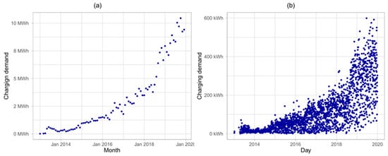
Figure 1.
(a) Charging demand in all stations each month, (b) Charging demand in all stations each day.
In addition to rise in daily energy demand, Figure 2 shows the energy demand per session has risen over the course of the study as well. Although there are still many sessions that do not have a large energy usage, the overall trend shows that more PEVs are beginning to use more energy. With the rapid penetration of the Tesla 3 and other new modern vehicles with larger batteries, the upper limit for energy used in a single charging session is rising. This trend may also be affected by behavioral factors, such as decreased user range anxiety, or the willingness to drive longer distances between charging sessions.
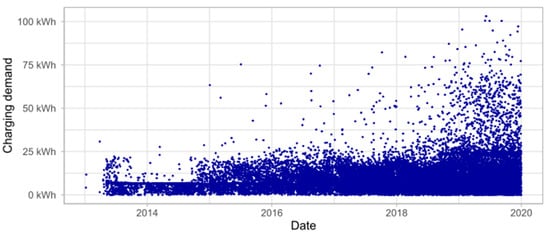
Figure 2.
Charging demand for every session.
The subsequent analysis in this research focuses on the energy demand of each charging session, rather than aggregate demand over some period of time, or multiple locations. While knowledge of daily or hourly demand is important at the utility level, anticipation of individual session demand is important at the charging station level, as well as for applications, discussed in Section 2, such as scheduling and vehicle-to-grid integration. In addition, predictions of session behavior can be combined with predictions about the temporal and spatial distribution of sessions in area to generate daily demand predictions.
In order to more accurately analyze and predict trends in charging behavior, several data points were removed from the set. In total, 8.5% of the total sessions used 0 kWh, indicating connection errors or technical problems with the stations. In addition, in order to focus on the trends of long-term PEV use and avoid overfitting the data, sessions from users who charged less than 10 times over the course of the study were omitted. After cleaning, the final dataset consisted of 22,231 charging sessions. Figure 3 shows the histogram of charging demand per session, at 1 kWh intervals.
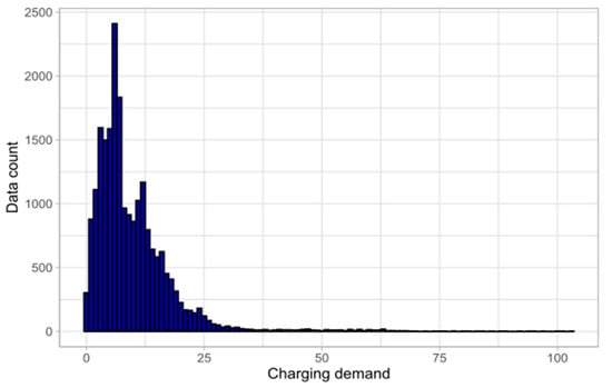
Figure 3.
Histogram of charging demand per session, at 1 kWh intervals.
For each charging session, a total of twelve parameters are used to predict the charging demand . These parameters were chosen from a combination of what information was available in the data, and what features have been hypothesized to be correlated to demand, or shown to be correlated in research on other datasets discussed in Section 2.
First, the location category of the station as four groups: Education (universities and schools), which included a total of 14 ports; Workplace (charging stations owned by companies), with 4 ports; Shopping Center (malls and other retail centers), with 4 ports; Public Parking (downtown and other public parking lots), with 75 ports. Note that the cumulative port count for each group is the count as of 2019. Four different time variables are considered; a numeric time series () describing the absolute time, a numeric time of day , and two categorical variables indicating the season and day of week. Fee policy ( indicates whether the session was free or paid. Port number ( is included as each station may have up to two ports.
The unique user ID is not used as a variable, in order to explore the dependence of energy demand on available statistics of an arbitrary user, rather than find a functional relationship specific to each user. This approach potentially yields lower accuracy than user-specific modeling, but is much more easily generalized to large populations, fast enough for real-time prediction applications, and allows for the exploration of charging behavior patterns that are common between users. Instead, for each session, statistics are calculated about the past behavior of each user: the mean energy, the maximum energy (, the minimum energy , the number of previous sessions , and the time in days since the last session ended . The prediction of charging demand can, thus, be expressed as a function of these twelve parameters, shown in Equation (1) and Table 2:

Table 2.
Parameters of interest for each charging session.
Figure 4 displays the distribution of the charging sessions over several categories of interest. Figure 4a shows the amount of sessions that began on each day of the week. It is apparent that there is a significant drop in public charging usage on Saturday and Sunday compared with the weekdays, which could show that most electric vehicles in this study are used for commuting to and from work. Figure 4b shows that port number two (on the right side, facing the wall) was used 19.6% more often than port number one. Figure 4c shows the distribution by time of day; 89.7% of the total sessions occurred between 6 a.m. and 6 p.m. Figure 4d shows that free stations were utilized 32.8% more than paid stations. In Figure 4e, slightly more sessions occur in summer and autumn that in spring and winter. Finally, Figure 4f shows that the majority of the charging sessions in this study come from public parking lots.
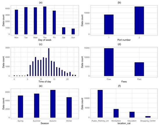
Figure 4.
Histogram of sessions by (a) Day of Week, (b) Port Number, (c) Time of Day, (d) Fees Policy, (e) Seasons, and (f) Location category.
4. Charging Demand Prediction Framework
The objective of this research is to assess the feasibility of predicting the energy demand of a charging session, using only information available at the start of charging. If this energy demand is assumed to be a function of the twelve input parameters in Equation (1), the inputs and outputs of this function are known for every session in the dataset. Regression analysis can then be used to approximate an underlying function that maps a given set of input parameters (the information known at charging) to the output parameter (the recorded energy demand). This approximated function (model) can then be used to predict the energy demand of future sessions, based on the input parameters of those sessions. The overall framework is illustrated in Figure 5.
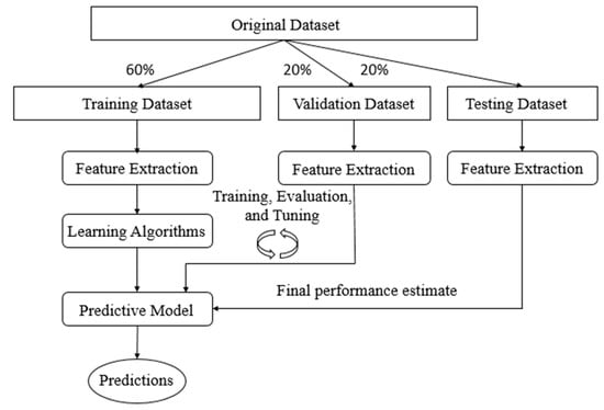
Figure 5.
Charging Demand Prediction framework.
There are many established regression techniques, with various advantages and disadvantages. Because the prediction of session energy demand has possible real-time applications, three machine learning algorithms with a balance of accuracy and computational speed are investigated: Gradient Boosting (XGBoost), Random Forest (RF), and Support Vector Machine (SVM). The following subsection explains more about the methods used in this research.
In addition to the machine learning methods, a linear regression, typically the fastest and least accurate, is performed for reference. For this method, Equation (1) for is simply assumed to be linear, with each input parameter having its own constant coefficient. The appropriate coefficients are derived by finding the linear relationship that best fits the energy demand’s dependence on each input parameter.
4.1. Machine Learning Methods
1. Gradient Boosting
Boosting frameworks are often chosen due to their effortlessness and extraordinary outcomes on average size datasets. XGBoost, in particular, has seen widespread use in data science due to its high accuracy, flexibility, speed, and efficiency [47]. It is used to solve regression, classification, and ranking problems [48]. XGBoost’s concept is to improve the performance of computational power for boosted tree algorithms. This algorithm is considered to be one of the fastest to incorporate tree ensemble approaches, using information from all data points in a leaf to decrease the search space of potential feature splits [46,49].
2. Random Forest (RF)
Random forests, also known as random decision forests, are a highly utilized ensemble training method. It is commonly applied for both classification and regression and functions by building an aggregation of decision trees at training time and outputting the class that is the mode of the classes (classification) or mean prediction (regression) of the individual trees’ leverage [50]. Ensemble methods use multiple learning models to gain better predictive results. In the case of a random forest, the model creates an entire forest of random uncorrelated decision trees to arrive at the best possible answer. Random forest aims to overcome the correlation issue by picking only a subsample of the feature space at each split. Fundamentally, it aims to decorrelate the trees and cut the trees by setting stopping criteria for node splits. The random forest algorithm offers an excellent accuracy among current algorithms, and runs efficiently on large datasets. It can manipulate thousands of input variables without variable deletion. It creates an inner straight estimate of the generalization error as the forest building progresses [51].
3. Support Vector Machine (SVM)
Commonly, support vector machines are recognized as a classification method; however, they can be used in both classification and regression problems. It can simply manipulate various, continuous, and categorical variables. SVMs build a hyperplane in multidimensional space to separate different classes, creating an optimal hyperplane through an iterative process, which is applied to reduce the error. The ultimate output of SVM is a maximum marginal hyperplane that best separates the dataset into classes. SVMs offer very high accuracy compared to other classifiers such as logistic regression and decision trees. It is known for its kernel trick to handle nonlinear input spaces and is used in a variety of applications such as face detection, intrusion detection, classification of emails, and handwriting recognition [52].
For the purpose of generating a predictive model of this dataset, SVM (regression) can be considered a direct improvement to linear regression, with slack variables introduced to cope with infeasible constraints [53].
4.2. Machine Learning Methods’ Accuracy Evaluations
A model’s accuracy is evaluated by examining the differences between the predictions of the model and the actual observations in the test set. Because there are thousands of observations in the test set, these differences are summarized by common statistical evaluation metrics, and these metrics are compared for each of the four regression methods. The following subsection explains more about the evaluation metrics used in this research:
1. Coefficient of determination (R2)
R2 is an important performance metric for any regression analysis. Used in statistical models for many applications, it provides a quantification of how well the model predicts the relationship between the input data and the generated output. A model that always generates a perfect prediction would have an R2 of one, while a model whose predictions do not respond at all to input parameters would have an R2 of zero.
Formally, R2 is defined by Equation (2), where the numerator is the sum of squares of the residuals (), divided by the sum of squares for the test set . This can also be understood as a ratio of variances, indicating what portion of the variance in the result is accurately predicted by the model.
where, is the actual value from the test set, is the predicted value of , and is the mean of the values.
2. Root Mean Square Error (RMSE)
Root Mean Square Error (RMSE) is another common statistical metric, quantifying the average amount of error between a prediction and a test set. RMSE has the same units as the variable being predicted. It is defined by Equation (3) and is simply the standard deviation of the residuals or errors. RMSE provides information on how far, on average, a model’s predictions are from their expected values.
where n is the number of observations.
3. Mean Absolute Error (MAE)
Like the RMSE, mean absolute error (MAE) is also commonly used to quantify the average amount of error between a prediction and a test set. Instead of calculating the standard deviation of residuals, the MAE is simply the average of the absolute value of the residuals, as seen in Equation (4). While RMSE and MAE are similar, RMSE gives a higher weight to larger errors before averaging. When the MAE is significantly lower than the RMSE, it can indicate a larger spread in the values of the residuals.
4.3. Data Splitting
To perform the regression analysis, tune the model, and test the performance, the full dataset is divided into three subsets: Training, Validation, and Test. The choice of which set to place each session in is important, as this determines which sessions the model learns from, and which sessions the model is tested on. A strict split by time, for instance, would create a model that learns from past behavior, and predicts future behavior. However, an extreme example could be considered where there are only two users in a dataset—one user charging from 2013 to 2018, and a different user charging in 2019. A model split by time might then only learn from one user, and make predictions for a different user with entirely different input parameters and energy demand. Therefore, to train the model in such a way that it learns from all users in the dataset, while still testing against ‘future’ behavior, the following steps are performed:
- Sort the dataset by user, and discard the first session from each user. This session is used as the starting point for calculating that user’s mean, max, and min energy demand of previous sessions, as well as the days since last charge.
- Place the first (chronologically) 60% of each user’s charging sessions into the training set.
- Place the next 20% of each user’s charging sessions into the validation set.
- Place the final 20% of each user’s charging sessions into the test set.
It is important to emphasize that this approach does not attempt to predict the behavior of a new, unknown user—rather, it isolates the question of whether each user’s future behavior can be predicted based on their past behavior (as well as other variables), having studied the past behavior of many users. In practice, this tests whether a dynamic implementation of this framework converges toward accurate prediction, given enough historical information of each user, rather than testing the model’s ability to predict the early sessions of a user.
In total, there are 13,115 sessions in the training set, 4405 in the validation set, and 4483 in the test set. Figure 6 displays the distribution of charging demands in each set, and Table 3 presents statistics of each set. It can be seen that the overall distribution of each set is relatively similar, with a slight increase in average demand in the validation and test sets. This increase is well below the overall increase in session demand over the course of the study, shown previously in Figure 2, indicating that while the average user in this study charges for slightly more energy the longer they use public charging stations, the majority of the increase in energy demand per session is due to new users and vehicles.
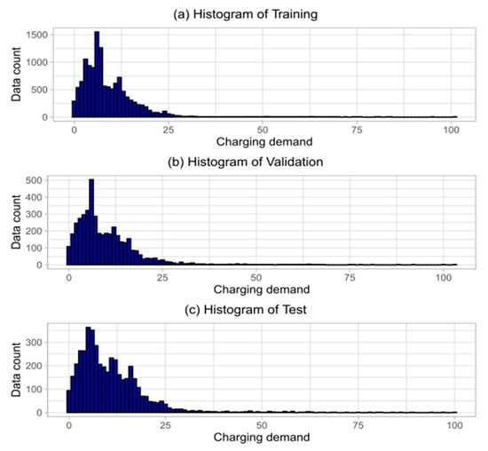
Figure 6.
Histograms of (a) Training, (b) Validation, and (c) Test sets, in 1 kWh increments.

Table 3.
Statistics of Training, Validation, and Test Sets, in kWh.
4.4. Model Training and Validation
The R programming language is used to implement each model. In addition, RStudio is the integrated development environment (IDE) utilized to organize the R code [54]. The Caret package [55] is used for the Linear, XGBoost, and SVM methods. However, the Ranger package [56] is used for Random Forest due to its speed.
Each regression method contains several tuning parameters. Proper tuning parameter selection is an important issue for predictive performance [57]. The validation set is used to test the performance of the model using different combinations of tuning parameters. The optimal tuning parameters for this framework and dataset are provided in Table 4.

Table 4.
Machine Learning Methods’ Tuning Parameters.
5. Charging Demand Prediction Results
The predicted and observed values in the test set are shown for each method in Figure 7. Figure 8 displays the residuals for each charging session prediction, with the indices sorted by user, and then, by time. Finally, Figure 9 displays the histograms for the residuals of each method, in 1 kWh increments.
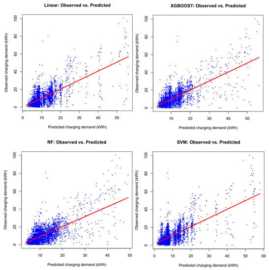
Figure 7.
Predicted vs. Observed values for each method.
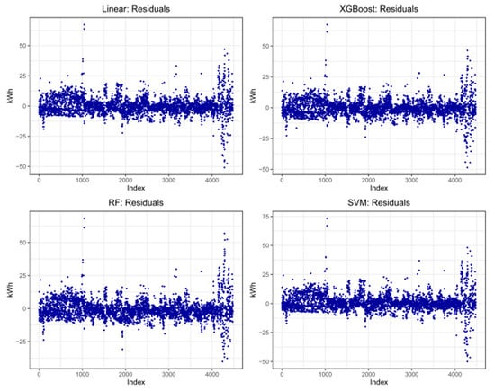
Figure 8.
Residuals for each method—indices are grouped by user, then time.
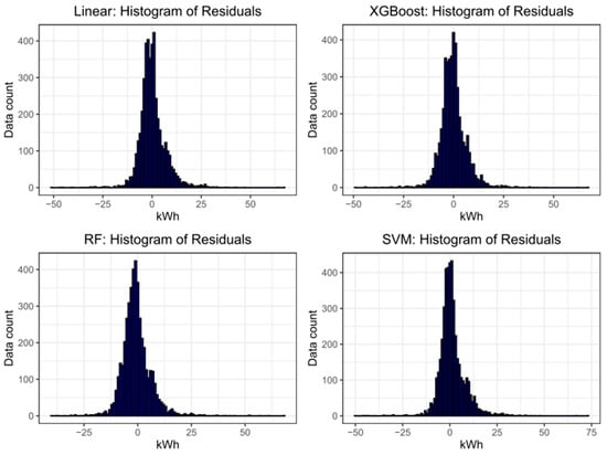
Figure 9.
Histograms for the residuals of each method, in 1 kWh increments.
The statistics of these results can be summarized using the standard metrics outlined in Section 4, as shown in Table 5, for both the test and validation cases. For ease of comparison, these same metrics are plotted in Figure 10.

Table 5.
Accuracy Metrics for Each Method, in kWh.
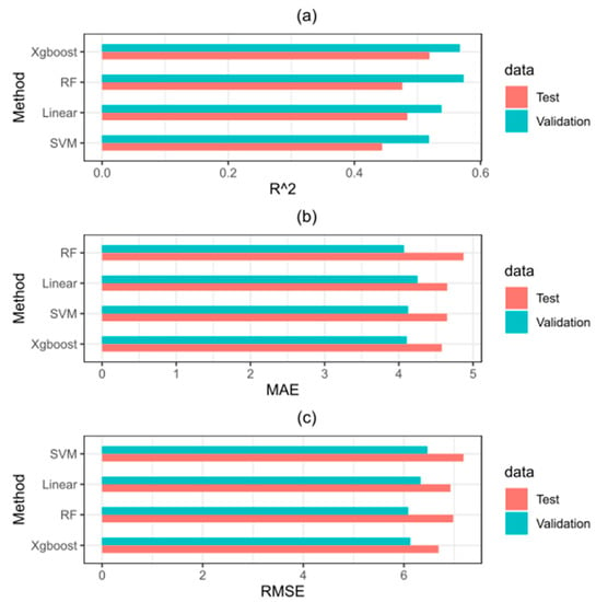
Figure 10.
Accuracy metric comparisons including (a) R2, (b) MAE, and (c) RMSE for each method.
Of the methods explored in this study, XGBoost yields the most accurate predictions, with an R2 of 0.519, a mean absolute error of 4.57 kWh, and an RMSE of 6.68 kWh. This value of R2 indicates that nearly 50% of the variance in the test data is unaccounted for by the model. As the mean energy demand in the test data is 10.95 kWh, the MAE is roughly 42% of the average demand. As discussed in Section 4.2, the fact that the RMSE is significantly higher than the MAE indicates that there is a large spread in the residuals, as can be seen in Figure 8 and Figure 9.
The visible gaps between high kWh predicted values in the linear and SVM cases in Figure 7 indicate that for sessions with high predicted energy demand, the predictions of these methods are clustered around certain values. These values are the average demands of the small number of users that charged for large amounts, indicating that these methods did not make predictions far from the user means.
The choice of sorting the residuals in Figure 8 by user illustrates some important information. The prediction error for the last users in the set are much larger than those of most users. This is not simply due to less available data for these users, as they had a similar total number of sessions to the majority of users studied, rather their charging behavior was more erratic than other users in the study, and not well correlated to any of the available features. The sessions of these users make up about 7% of the sessions in the study—omitting them from the test set and using the predictions of XGBoost indicates that for 93% of the users, the model has an R2 of 0.61, and MAE of 4.19 kWh, and an RMSE of 5.75 kWh, a significant increase in accuracy. In practice of course, without any further identifying information about such anomalous users or a correlation between this behavior and some known input parameter, there is no way to distinguish them. For the purpose of assessing the feasibility of session energy prediction, it is important not to consider such sessions ‘outliers’, but the relatively higher prediction accuracy for 93% of sessions is worth noting.
To further understand the relationship between the charging demand and the 12 variables used to classify each charging session, the feature dependence of each model can be analyzed. Figure 11 illustrates the relative importance of each variable in predicting charging demand (using the nomenclature in Table 2), for each method.
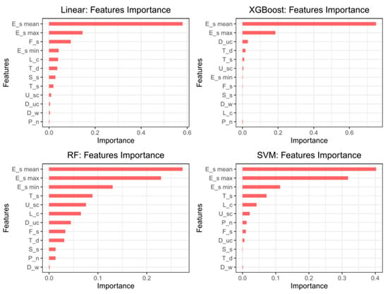
Figure 11.
Feature importance comparisons for each method.
For all four methods, the most significant predictor of charging demand is the user’s average demand for past sessions. Excluding this variable from the model (which could be necessary if it is not available, or to predict the charging demand of a new user) results in a much less accurate prediction [6]. The second most important variable for each method is the user’s maximum demand in past sessions. In addition to providing a ceiling for prediction, for many users, this variable is somewhat correlated with mean demand. The relative importance of the remaining variables varies significantly for each method. For Random Forest, the minimum past demand, absolute time, and user session count contribute significantly, and all features except day of week have a visible effect on the prediction. This is partially due to Random Forest’s tendency to follow the training data too closely, or overfit, as many of these features were not important in other methods. It is noteworthy that for the most accurate method, XGBoost, the feature importance drops off sharply after the maximum past demand, followed distantly by the days since last charge and time of day. Time of day, in particular, has been noted in past research to have some correlation to both energy demand and idle time [6,35], but in this dataset, the dependence is very weak. It should be noted that while many of the above features are not correlated well to demand, their exclusion from the model also does not significantly affect prediction accuracy, so they are preserved in the presented results to illustrate their relative importance.
One implication of these results is that, from the definition of R2, roughly 48% of the variance in charging demand by session cannot be accounted for by the aforementioned variables—rather, it represents the remaining ‘randomness’ in user behavior. More precisely, it indicates that the energy demand of an arbitrary session is a function of far more variables than are considered here, because it is information that will never be available to a charging station. Examples include all factors that might influence parking behavior at any of the public stations in this study, as well as driving behavior between recorded sessions. Nevertheless, all four prediction methods, XGBoost in particular, but linear regression as well, offer predictions of reasonable accuracy for many users.
6. Conclusions and Future Work
In analyzing the charging behavior of PEV users, the dependence of charging session consumption on various user and session features is explored using a data-driven energy prediction framework. Accurate prediction of session charging demand has many possible applications, including scheduling [58,59,60], grid stability [61,62], and smart grid integration [63,64]. By formulating the energy prediction as a multiple regression problem, several statistical machine learning regression methods are applied to predict how much energy the PEV user will consume after plugging-in. This approach is validated using a dataset collected from public charging stations in the state of Nebraska.
The results show that the regression algorithm, XGBoost, outperforms the other algorithms in predicting energy consumption, but all methods offer only moderate accuracy, accounting for roughly 50% of the variance in user behavior. In this dataset, the primary statistic of predictive value is the user’s average demand for past sessions, and a large portion of the predictive error is concentrated in a small portion of erratic users.
While in this study, the predictive framework has been applied ambitiously to data from many different stations, the same framework could be applied to data from a smaller area or even a single station, in which it is possible that the input parameters have an even higher correlation to the energy demand, resulting in better predictions for a smaller subset of users. The feature space considered is small enough, and the algorithms fast enough, for implementation in a dynamic real-time model that continually learns from user behavior and updates future predictions.
A hurdle in this research is the analysis of a large amount of semi-random data, which leads to difficulties in finding a predictive model to describe the charging and parking behaviors. Further analysis can be performed with other regression models, deep learning, and neural networks. Analysis of input parameters not currently recorded by charging point operators could yield new correlations between user behaviors and charging demand. An extension to this work can be done by analyzing the charging behavior in both public and residential charging stations. V2G technique could be applied to manage the electric grid and customer energy use during peak demand using the predicted energy values.
Author Contributions
Conceptualization, A.A.; Methodology; Software, A.A.; M.R.; Supervision, M.A.; Writing—original draft, A.A. and F.A.; Writing—review and editing, K.J. All authors have read and agreed to the published version of the manuscript.
Funding
This project was funded by The Nebraska Environmental Trust (NET)/the Nebraska Community Energy Alliance (NCEA), grant number 19-125, Internal funding from the Durham School of Architectural Engineering and Construction.
Acknowledgments
This work has been supported in part by the Nebraska Environmental Trust (NET), the Nebraska Community Energy Alliance (NCEA), and the Durham School of Architectural Engineering and Construction—University of Nebraska-Lincoln.
Conflicts of Interest
The authors declare no conflict of interest.
References
- Rabe, B.G. Beyond Kyoto: Climate change policy in multilevel governance systems. Governance 2007, 20, 423–444. [Google Scholar] [CrossRef]
- Dimitrov, R.S. The Paris agreement on climate change: Behind closed doors. Glob. Environ. Polit. 2016, 16, 1–11. [Google Scholar] [CrossRef]
- Silva, C.; Ross, M.; Farias, T. Evaluation of energy consumption, emissions and cost of plug-in hybrid vehicles. Energy Convers. Manag. 2009, 50, 1635–1643. [Google Scholar] [CrossRef]
- Coffman, M.; Bernstein, P.; Wee, S. Electric vehicles revisited: A review of factors that affect adoption. Transp. Rev. 2017, 37, 79–93. [Google Scholar] [CrossRef]
- Rezvani, Z.; Jansson, J.; Bodin, J. Advances in consumer electric vehicle adoption research: A review and research agenda. Transp. Res. Part D Transp. Environ. 2015, 34, 122–136. [Google Scholar] [CrossRef]
- Almaghrebi, A. The Impact of PEV User Charging Behavior in Building Public Charging Infrastructure; University of Nebraska-Lincoln: Lincoln, NE, USA, May 2020. [Google Scholar]
- Yusuf, J.; Hasan, A.S.M.J.; Ula, S. Impacts of Plug-in Electric Vehicles on a Distribution Level Microgrid. 51st N. Am. Power Symp. NAPS 2019, 2019, 1–6. [Google Scholar] [CrossRef]
- Tayarani, H.; Jahangir, H.; Nadafianshahamabadi, R.; Golkar, M.A.; Ahmadian, A.; Elkamel, A. Optimal charging of plug-in electric vehicle: Considering travel behavior uncertainties and battery degradation. Appl. Sci. 2019, 9, 3420. [Google Scholar] [CrossRef]
- Noussan, M.; Neirotti, F. Cross-country comparison of hourly electricity mixes for EV charging profiles. Energies 2020, 13, 2527. [Google Scholar] [CrossRef]
- Yang, Z.; Li, K.; Niu, Q.; Xue, Y. A comprehensive study of economic unit commitment of power systems integrating various renewable generations and plug-in electric vehicles. Energy Convers. Manag. 2017, 132, 460–481. [Google Scholar] [CrossRef]
- Yang, Z.; Li, K.; Niu, Q.; Xue, Y.; Foley, A. A self-learning TLBO based dynamic economic/environmental dispatch considering multiple plug-in electric vehicle loads. J. Mod. Power Syst. Clean Energy 2014, 2, 298–307. [Google Scholar] [CrossRef]
- Yang, Z.; Li, K.; Foley, A. Computational scheduling methods for integrating plug-in electric vehicles with power systems: A review. Renew. Sustain. Energy Rev. 2015, 51, 396–416. [Google Scholar] [CrossRef]
- Shuaib, K.; Barka, E.; Abdella, J.A.; Sallabi, F.; Abdel-Hafez, M.; Al-Fuqaha, A. Secure plug-in electric vehicle (PEV) Charging in a smart grid network. Energies 2017, 10, 1024. [Google Scholar] [CrossRef]
- Amjad, M.; Ahmad, A.; Rehmani, M.H.; Umer, T. A review of EVs charging: From the perspective of energy optimization, optimization approaches, and charging techniques. Transp. Res. Part D Transp. Environ. 2018, 62, 386–417. [Google Scholar] [CrossRef]
- Hardman, S.; Jenn, A.; Tal, G.; Axsen, J.; Beard, G.; Daina, N.; Figenbaum, E.; Jakobsson, N.; Jochem, P.; Kinnear, N.; et al. A review of consumer preferences of and interactions with electric vehicle charging infrastructure. Transp. Res. Part D Transp. Environ. 2018, 62, 508–523. [Google Scholar] [CrossRef]
- Painuli, S.; Rawat, M.S.; Rayudu, D.R. A Comprehensive Review on Electric Vehicles Operation, Development and Grid Stability. In Proceedings of the 2018 International Conference on Power Energy, Environment and Intelligent Control (PEEIC), Greater Noida, India, 13–14 April 2018; pp. 807–814. [Google Scholar] [CrossRef]
- Shaukat, N.; Khan, B.; Ali, S.M.; Mehmood, C.A.; Khan, J.; Farid, U.; Majid, M.; Anwar, S.M.; Jawad, M.; Ullah, Z. A survey on electric vehicle transportation within smart grid system. Renew. Sustain. Energy Rev. 2018, 81, 1329–1349. [Google Scholar] [CrossRef]
- Moon, H.; Park, S.Y.; Jeong, C.; Lee, J. Forecasting electricity demand of electric vehicles by analyzing consumers’ charging patterns. Transp. Res. Part D Transp. Environ. 2018, 62, 64–79. [Google Scholar] [CrossRef]
- Rahman, S.; Shrestha, G.B. An investigation into the impact of electric vehicle load on the electric utility distribution system. IEEE Trans. Power Deliv. 1993, 8, 591–597. [Google Scholar] [CrossRef]
- Neaimeh, M.; Wardle, R.; Jenkins, A.M.; Yi, J.; Hill, G.; Lyons, P.F.; Hübner, Y.; Blythe, P.T.; Taylor, P.C. A probabilistic approach to combining smart meter and electric vehicle charging data to investigate distribution network impacts. Appl. Energy 2015, 157, 688–698. [Google Scholar] [CrossRef]
- Mao, D.; Gao, Z.; Wang, J. An integrated algorithm for evaluating plug-in electric vehicle’s impact on the state of power grid assets. Electr. Power Energy Syst. 2019, 105, 793–802. [Google Scholar] [CrossRef]
- Hong, S.K.; Lee, S.G.; Kim, M. Assessment and mitigation of electric vehicle charging demand impact to transformer aging for an apartment complex. Energies 2020, 13, 2571. [Google Scholar] [CrossRef]
- Mies, J.J.; Helmus, J.R.; van den Hoed, R. Estimating the charging profile of individual charge sessions of Electric Vehicles in the Netherlands. World Electr. Veh. J. 2018, 9, 17. [Google Scholar] [CrossRef]
- Shao, S.; Pipattanasomporn, M.; Rahman, S. Challenges of PHEV penetration to the residential distribution network. In Proceedings of the 2009 IEEE Power & Energy Society General Meeting, Calgary, AB, Canada, 26–30 July 2009; pp. 1–8. [Google Scholar] [CrossRef]
- Xing, Q.; Chen, Z.; Zhang, Z.; Xu, X.; Zhang, T.; Huang, X.; Wang, H. Urban Electric Vehicle Fast-Charging Demand Forecasting Model Based on Data-Driven Approach and Human Decision-Making Behavior. Energies 2020, 13, 1412. [Google Scholar] [CrossRef]
- Liu, G.; Kang, L.; Luan, Z.; Qiu, J.; Zheng, F. Charging station and power network planning for integrated electric vehicles (EVs). Energies 2019, 12, 2595. [Google Scholar] [CrossRef]
- Yagcitekin, B.; Uzunoglu, M. A double-layer smart charging strategy of electric vehicles taking routing and charge scheduling into account. Appl. Energy 2016, 167, 407–419. [Google Scholar] [CrossRef]
- Sallabi, F.; Shuaib, K.; Alahmad, M. Online scheduling scheme for smart electric vehicle charging infrastructure. In Proceedings of the 2017 13th International Wireless Communications and Mobile Computing Conference, IWCMC, Valencia, Spain, 26–30 June 2017; pp. 1297–1302. [Google Scholar] [CrossRef]
- Ghotge, R.; Snow, Y.; Farahani, S.; Lukszo, Z.; van Wijk, A. Optimized scheduling of EV charging in solar parking lots for local peak reduction under EV demand uncertainty. Energies 2020, 13, 1275. [Google Scholar] [CrossRef]
- Mao, T.; Zhang, X.; Zhou, B. Intelligent Energy Management Algorithms for EV-charging Scheduling with Consideration of Multiple EV Charging Modes. Energies 2019, 12, 265. [Google Scholar] [CrossRef]
- Zima-Bockarjova, M.; Sauhats, A.; Petrichenko, L.; Petrichenko, R. Charging and Discharging Scheduling for Electrical Vehicles Using a Shapley-Value Approach. Energies 2020, 13, 1160. [Google Scholar] [CrossRef]
- Weiller, C. Plug-in hybrid electric vehicle impacts on hourly electricity demand in the United States. Energy Policy 2011, 39, 3766–3778. [Google Scholar] [CrossRef]
- Ashtari, A.; Bibeau, E.; Shahidinejad, S.; Molinski, T. PEV charging profile prediction and analysis based on vehicle usage data. IEEE Trans. Smart Grid 2011, 3, 341–350. [Google Scholar] [CrossRef]
- Foley, A.; Tyther, B.; Calnan, P.; Gallachóir, B.Ó. Impacts of electric vehicle charging under electricity market operations. Appl. Energy 2013, 101, 93–102. [Google Scholar] [CrossRef]
- Wolbertus, R.; Kroesen, M.; van den Hoed, R.; Chorus, C. Fully charged: An empirical study into the factors that in fl uence connection times at EV-charging stations. Energy Policy 2018, 123, 1–7. [Google Scholar] [CrossRef]
- Almaghrebi, A.; al Juheshi, F.; Nekl, J.; James, K.; Alahmad, M. Analysis of Energy Consumption at Public Charging Stations, A Nebraska Case Study. In Proceedings of the 2020 IEEE Transportation Electrification Conference & Expo (ITEC), Chicago, IL, USA, 22–26 June 2020; pp. 1–6. [Google Scholar] [CrossRef]
- Almaghrebi, A.; Shom, S.; al Juheshi, F.; James, K.; Alahmad, M. Analysis of user charging behavior at public charging stations. In Proceedings of the 2019 IEEE Transportation Electrification Conference and Expo (ITEC), Novi, MI, USA, 19–21 June 2019; pp. 1–6. [Google Scholar] [CrossRef]
- Babrowski, S.; Heinrichs, H.; Jochem, P.; Fichtner, W. Load shift potential of electric vehicles in Europe. J. Power Sources 2014, 255, 283–293. [Google Scholar] [CrossRef]
- Schäuble, J.; Kaschub, T.; Ensslen, A.; Jochem, P.; Fichtner, W. Generating electric vehicle load profiles from empirical data of three EV fleets in Southwest Germany. J. Clean. Prod. 2017, 150, 253–266. [Google Scholar] [CrossRef]
- Straka, M.; De Falco, P.; Ferruzzi, G.; Proto, D.; Van Der Poel, G.; Khormali, S.; Buzna, L. Predicting popularity of electric vehicle charging infrastructure in urban context. IEEE Access 2020, 8, 11315–11327. [Google Scholar] [CrossRef]
- Fotouhi, Z.; Hashemi, M.R.; Narimani, H.; Bayram, I.S. A General Model for EV Drivers’ Charging Behavior. IEEE Trans. Veh. Technol. 2019, 68, 7368–7382. [Google Scholar] [CrossRef]
- Brady, J.; O’Mahony, M. Modelling charging profiles of electric vehicles based on real-world electric vehicle charging data. Sustain. Cities Soc. 2016, 26, 203–216. [Google Scholar] [CrossRef]
- Kelly, J.C.; Macdonald, J.S.; Keoleian, G.A. Time-dependent plug-in hybrid electric vehicle charging based on national driving patterns and demographics. Appl. Energy 2012, 94, 395–405. [Google Scholar] [CrossRef]
- Chen, L.; Huang, X.; Zhang, H. Modeling the charging behaviors for electric vehicles based on ternary symmetric kernel density estimation. Energies 2020, 13, 1551. [Google Scholar] [CrossRef]
- Chung, Y.W.; Khaki, B.; Li, T.; Chu, C.; Gadh, R. Ensemble machine learning-based algorithm for electric vehicle user behavior prediction. Appl. Energy 2019, 254, 113732. [Google Scholar] [CrossRef]
- Lucas, A.; Barranco, R.; Refa, N. EV Idle Time Estimation on Charging Infrastructure, Comparing Supervised Machine Learning Regressions. Energies 2019, 12, 269. [Google Scholar] [CrossRef]
- Chen, T.; Guestrin, C. XGBoost: A Scalable Tree Boosting System. In Proceedings of the 22nd Acm Sigkdd International Conference on Knowledge Discovery and Data Mining, San Francisco, CA, USA, 13–17 August 2016; pp. 785–794. [Google Scholar]
- Fathabadi, H. Plug-in hybrid electric vehicles: Replacing internal combustion engine with clean and renewable energy based auxiliary power sources. IEEE Trans. Power Electron. 2018, 33, 9611–9618. [Google Scholar] [CrossRef]
- Choi, D.K. Data-Driven Materials Modeling with XGBoost Algorithm and Statistical Inference Analysis for Prediction of Fatigue Strength of Steels. Int. J. Precis. Eng. Manuf. 2019, 20, 129–138. [Google Scholar] [CrossRef]
- Ho, T.K. Random decision forests. In Proceedings of the 3rd International Conference on Document Analysis and Recognition, Montreal, QC, Canada, 14–16 August 1995; pp. 278–282. [Google Scholar]
- Hastie, T.; Tibshirani, R.; Friedman, J. The Elements of Statistical Learning: Data Mining, Inference, and Prediction; Springer Science & Business Media: Berlin, Germany, 2009. [Google Scholar]
- Alsaleem, F.; Tesfay, M.K.; Rafaie, M.; Sinkar, K.; Besarla, D.; Arunasalam, P. An IoT Framework for Modeling and Controlling Thermal Comfort in Buildings. Front. Built Environ. 2020, 6, 1–14. [Google Scholar] [CrossRef]
- Smola, A.J.; Schölkopf, B. A tutorial on support vector regression. Stat. Comput. 2004, 14, 199–222. [Google Scholar] [CrossRef]
- RStudio Team. Integrated Development Environment for R. 2012. Available online: http://www.rstudio.com/ (accessed on 4 June 2020).
- Kuhn, M.; Wing, J.; Weston, S.; Williams, A.; Keefer, C.; Engelhardt, A.; Cooper, T.; Mayer, Z.; Kenkel, B.; Team, R.C.; et al. Package ‘caret’. R J. 2020. Available online: http://cran.r-project.org/web/packages/caret/caret.pdf (accessed on 15 August 2020).
- Wright, M.N.; Wager, S.; Probst, P. A Fast Implementation of Random Forests. R package version 0.11. 2019. Available online: https://cran.r-project.org/web/packages/ranger/index.html (accessed on 15 August 2020).
- Ebrahimifakhar, A.; Kabirikopaei, A.; Yuill, D. Data-driven fault detection and diagnosis for packaged rooftop units using statistical machine learning classification methods. Energy Build. 2020, 225, 110318. [Google Scholar] [CrossRef]
- Srithapon, C.; Ghosh, P.; Siritaratiwat, A.; Chatthaworn, R. Optimization of electric vehicle charging scheduling in urban village networks considering energy arbitrage and distribution cost. Energies 2020, 13. [Google Scholar] [CrossRef]
- Choi, B.G.; Oh, B.C.; Choi, S.; Kim, S.Y. Selecting Locations of Electric Vehicle Charging Stations Based on the Traffic Load Eliminating Method. Energies 2020, 13. [Google Scholar] [CrossRef]
- Lee, J.; Lee, E.; Kim, J. Electric Vehicle Charging and Discharging Algorithm Based on Reinforcement Learning with Data-Driven Approach in Dynamic Pricing Scheme. Energies 2020, 13. [Google Scholar] [CrossRef]
- Kim, D.J.; Ryu, K.S.; Ko, H.S.; Kim, B. Optimal Operation Strategy of ESS for EV Charging Infrastructure for Voltage Stabilization in a Secondary Feeder of a Distribution System. Energies 2020, 13. [Google Scholar] [CrossRef]
- Zweistra, M.; Janssen, S.; Geerts, F. Large scale smart charging of electric vehicles in practice. Energies 2020, 13. [Google Scholar] [CrossRef]
- Salvatti, G.A.; Carati, E.G.; Cardoso, R.; da Costa, J.P.; de Oliveira Stein, C.M. Electric vehiclesenergy management with V2G/G2V multifactor optimization of smart grids. Energies 2020, 13, 1191. [Google Scholar] [CrossRef]
- Cao, C.; Wu, Z.; Chen, B. Electric Vehicle–Grid Integration with Voltage Regulation in Radial Distribution Networks. Energies 2020, 13, 1802. [Google Scholar] [CrossRef]
© 2020 by the authors. Licensee MDPI, Basel, Switzerland. This article is an open access article distributed under the terms and conditions of the Creative Commons Attribution (CC BY) license (http://creativecommons.org/licenses/by/4.0/).