Article

Approximation Framework of Embodied Energy of Safety: Insights and Analysis

National Renewable Energy Laboratory, 15013 Denver West Parkway, Golden, CO 80401, USA
*
Author to whom correspondence should be addressed.
Energies 2020, 13(16), 4230; https://doi.org/10.3390/en13164230
Submission received: 15 June 2020 / Accepted: 12 August 2020 / Published: 16 August 2020
(This article belongs to the Section C: Energy Economics and Policy)

Abstract

:
Transportation safety, as a critical component of an efficient and reliable transportation system, has been extensively studied with respect to societal economic impacts by transportation agencies and policy officials. However, the embodied energy impact of safety, other than induced congestion, is lacking in studies. This research proposes an energy equivalence of safety (EES) framework to provide a holistic view of the long-term energy and fuel consequences of motor vehicle crashes, incorporating both induced congestion and impacts from lost human productivity resulting from injury and fatal accidents and the energy content resulting from all consequences and activities from a crash. The method utilizes a ratio of gross domestic product (GDP) to national energy consumed in a framework that bridges the gap between safety and energy, leveraging extensive studies of the economic impact of motor vehicle crashes. The energy costs per fatal, injury, and property-damage-only (PDO) crashes in gasoline gallon equivalent (GGE) in 2017 were found to be 200,259, 4442, and 439, respectively, which are significantly greater than impacts from induced congestion alone. The results from the motor vehicle crash data show a decreasing trend of EES per crash type from 2010 and 2017, due primarily in part to a decreasing ratio of total energy consumed to GDP over those years. In addition to the temporal analysis, we conducted a spatial analysis addressing national-, state-, and local-level EES comparisons by using the proposed framework, illustrating its applicability.

1. Introduction

Emerging technologies such as intelligent transportation systems, advanced driver-assistant systems, and connected and automated vehicles have been revolutionizing our mobility systems since the last decade. With respect to quantifying the impacts of emerging technology, enhanced mobility (decreased travel and increased accessibility and affordability), safety, and energy efficiency are the three pillars for evaluation. Safety is of paramount importance and underpins all other emerging aspects, as reflected in current American Association of State Highway Transportation Officials (AASHTO) road design standards and the overarching authority of the National Highway Traffic Safety Administration (NHTSA) with respect to standards and design for automotive crash worthiness. Interconnections between mobility and safety have been extensively studied. For instance, assessing safe-following headway of connected and automated vehicles has been researched by many scholars [1,2,3]. However, the relationship between safety (as in hazard exposure) and energy has been seldom explored when compared to the economic costs of motor vehicle crashes that have been studied for decades, either via empirical crash data or theoretical analysis (e.g., safety surrogate assessment model [4]). In the commercial sphere, automotive manufacturers weigh safety-oriented technologies much heavier than energy-consumption or energy-saving techniques, as liability is correlated primarily to failure of due diligence of design and manufacturing with respect to owner/occupant safety. To date, energy-beneficial technologies have been evaluated on a vehicle-efficiency level, which primarily pertains to the fuel consumption and emission resulting from enhanced fuel economy (miles per gallon), smoother traffic flow, and other cooperative driving technologies (e.g., platooning). Although macrolevel energy assessments have been touched, such as the impact of adaptive cruise control or cooperative–adaptive cruise control on traffic flow, and the reduction in nonrecurring congestion (and associated fuel use) if accident rates decreased, the overall connections between safety (that is, accident rates and hazard exposure), energy, and sustainability—encompassing all embodied energy—have not been fully evaluated. Embodied energy includes energy-related consequences apart from traffic dynamics, which includes the energy of all induced activities from a crash, embodied energy associated with longer-term impacts of reduced human productivity from injury and fatal injuries, and the “willingness to pay” to avoid such consequences.
The economic and societal costs of motor vehicle crashes have been reported. For example, a U.S. national motor vehicle crashes economic cost estimation was delivered by exploring a variety of crash report data sources, such as the “Traffic Safety Facts Annual Report” [5], which is published annually by NHTSA. In Canada, a crash economic study for Alberta province with 2007 data demonstrated that a fatal crash costs the equivalent of about CAD 7.2 million (Canadian dollars, 2007 value) [6]. These studies detailed the comprehensive economic cost of motor vehicle crashes, which can be considered as references for the energy assessment of crashes in the framework proposed herein. In an initial research framework to establish the energy equivalent of safety [7], a 2010 NHTSA study of economic impacts of various crash types was used as the basis for estimating energy impacts. Unlike the widely discussed economic cost of safety, the research on energy equivalence of safety (EES) (that is, the energy equivalent for various types of motor vehicle crashes) is rarely found. This paper proposes an energy approximation framework, building on the previous contribution, to quantify the EES and analyze the changes of EES across multiple years and jurisdictions in the U.S. The proposed gross domestic product (GDP)-weighted approximation framework and the energy analyses have the following properties:
  • Provides a holistic view of the long-term energy and fuel consequences of motor vehicle crashes, taking into account not only induced congestion and induced vehicle miles traveled (VMT), but also the consequence of the energy impact of induced activities (emergency response, health care, rehabilitation, vehicle repair), longer-term consequence of loss of human productivity, and society’s willingness to pay to avoid those consequences.
  • Develops an EES approximation model with temporal (multiple years) and spatial (various regional scales) dimensions considering the data availability.
  • Strengthens the connection between safety and energy for quantifying the overall performance of transportation systems. The latter is needed to understand that the ability of emerging technology to make transportation safer (without any improvement in traffic flow dynamics) also has a measurable energy impact.

2. Background and Data Preparation

2.1. Energy and Motor Vehicle Crashes

Research in energy and vehicle crashes can be broadly categorized into two levels: the vehicle level (and its subcomponents) and the traffic-flow level. In the event of a motor vehicle crash, the kinetic energy of the collision is in part transferred to vehicle occupants and passengers, who may suffer from injury if the energy exceeds a certain threshold [8,9], and the injury severity increases as the transferred kinetic energy increases [10], assuming other factors remain constant. The deformation and damage of the vehicle body to absorb kinetic energy have been crucial aspects of the passive safety of a vehicle [11]. The energy absorption has been achieved from the perspective of vehicle design (engine hood hinges [12]), geometric profile (circular tubes [13]), and material science (e.g., epoxy-based composite [14], magnesium alloy [15]).
Besides the vehicle-level analysis, another perspective is to study the wasted fuel at a traffic-flow level due to the congestion induced by the motor vehicle crashes, such as lane closures and the rubbernecking effect [16]. The “Urban Mobility Report” [17] uses traffic volume, speed, and the U.S. Environmental Protection Agency (EPA)’s Multi-scale mOtor Vehicle and equipment Emission System (MOVES) model [18] to estimate the CO2 emission and fuel consumption during congested conditions. Besides MOVES, other energy models that use second-by-second vehicle trajectory data (i.e., speed and acceleration) have been adopted, such as VT-Micro [19] and Future Automotive Systems Technology Simulator (FASTSim) [20]. A few studies have investigated traffic flow-level congestion impacts in the United States, where 5.5 billion hours are wasted annually because of both regular traffic congestion and induced congestion, translating to about USD 121 billion in 2012 [21]. In 2015, U.S. national congestion accounted for an additional 6.9 billion hours of driving and the equivalent of 3.1 billion gallons of fuel [17].
Apart from these national-level impacts of induced congestion from crashes, the research teams’ literature review did not uncover any direct linkage between per crash occurrence and resulting energy impacts, as is common for economic analyses. Using the national-level estimation of the energy consequences of induced congestion of 3.1 billion gallons of gasoline [17], and assuming 6.3 million crashes per year that cover fatal, injury, and property damage only (PDO) [5], the average per crash energy impact is estimated at 492 gallons of fuel per crash. Our framework indicates a much larger impact when all factors are taken into account. In terms of gasoline gallon equivalent (GGE), the fatal, injury, and PDO accidents account for 200,259, 4442, and 439 GGE in 2017, respectively.

2.2. Crash and Cost Composition

NHTSA has been documenting the details of motor crashes for decades. The National Automotive Sampling System (NASS) [22], established by NHTSA in 1979, comprised a General Estimate System (GES) [23] and a Crashworthiness Database System (CDS) [24]. GES and CDS were then replaced by the Crash Report Sampling System (CRSS) [25] and the Crash Investigation Sampling System (CISS) [26] in 2014 and 2016, respectively, as documented in “NHTSA’s Data Modernization Project” [27]. CRSS expands the police-reported accident report strata to pedestrian, motorcycle, and late-model vehicles. For CISS, the target population is all police-reported motor vehicle crashes on trafficways involving a passenger vehicle and in which a passenger vehicle is towed. Such requirements are different from CDS—its predecessor—which required damage as the reason for the towing.
Using the aforementioned data sets, NHTSA has published traffic safety facts since 1988 [5], which provide the annual crash numbers in three crash severity levels: fatal, injury, and PDO. Two crash severity measurement systems are commonly used in most studies: (1) AASHTO’s Highway Safety Manual (HSM) method, based on the KABCO scale, and (2) NHTSA’s method based on MAIS (Maximum Abbreviated Injury Scale) [21]. The KABCO scale is the most prevalent method used in police crash reports for assessing crash and injury severity. The coding in the KABCO scale assigns letter to each type of injury severity. In descending order in severity [28]:
  • (K): Fatal Injury
  • (A): Suspected serious injury
  • (B): Suspected minor injury
  • (C): Possible injury
  • (O): No apparent injury
Note that the descriptions in the KABCO scale entail uncertainty because the responding police officer generally does not have the requisite skill to medically determine the injury severity with great precision. The Abbreviated Injury Scale (AIS), on the other hand, was developed by the Association for the Advancement of Automotive Medicine to classify the injury severity for an individual. AIS provides an internationally accepted, anatomically based tool for measuring injury severity. MAIS is a score representing the most severe injury (using the AIS scale) on a single person in a crash [29]. As shown below, MAIS6 is the highest level, which represents unsurvivable injury, whereas MAIS1 represents minor injury.
  • (MAIS6): Unsurvivable injury
  • (MAIS5): Critical injury
  • (MAIS4): Severe injury
  • (MAIS3): Serious injury
  • (MAIS2): Moderate injury
  • (MAIS1): Minor injury
  • (MAIS0): No injury
Motor vehicle crash analysis is a crucial part of highway safety analysis in various countries. An international guideline distinguishes five components of crash cost: medical cost, production loss, human cost, property damage, and administrative costs [30]. In the United States, the HSM classifies crash costs into two types: direct costs and indirect costs [31] as shown in Table 1. The direct costs refer to the monetary costs that are directly attributable to crashes, such as property damage, human capital costs, medical costs, and induced congestion, all of which are relatively straightforward to estimate. The human capital cost measures a person’s contribution to the society through labor [6]. The indirect costs are measured in quality-adjusted life years (QALYs), which is a fraction of the value of a statistical life (VSL). VSL is the price that people are willing to pay to avoid the risk of death or injury [32]. In another words, QALY is a portion of the full VSL lost due to the crash. Additional discussion of VSL and its derivation and meaning are provided later. QALY is determined by the duration and severity of the health problem. For instance, the QALY value for the most serious injuries (with MAIS5 severity) is roughly 60% of a full remaining life. In comparison, minor injury (MAIS1) only accounts for 1% of a full remaining life. The relationships among the above concepts are illustrated in Figure 1.
It has been the standard practice for government agencies over the past three decades to use value of a statistical life to value risk [33]. VSL is often misinterpreted as referring to the “value of a life” rather than the value of small changes in one’s own mortality risks [34]. As such, “value of mortality risk” or “value of risk reduction” were proposed by some researchers to avoid misinterpretation [35]. The authors use “value of mortality risk” (VMR) henceforth to avoid such confusion. The Office of Management and Budget (OMB) provides recommendations for estimating VMR. Typically, the reduction of the mortality risk benefits account for the largest component of all new regulation benefits, especially for EPA and the U.S. Department of Transportation.
We included the example used in the final rule for Air Cargo Screening [36] from the Transportation Safety Agency to further illustrate the usage of VMR in government rule making. In the hypothetical and tragic scenario where an explosive device placed in cargo shipped on a standard narrow body passenger airplane during flight, the loss is assumed to be lives of all passengers and crewmembers on board, along with the destruction of the aircraft. For a plane with 114 passengers (average capacity 142 passenger and with a load factor of 80%) and 5 crewmembers, the estimated total VMR is approximately USD 714 million according to the VMR (USD 6 million per person) set forth by the USDOT. The total cost including the cost of the aircraft increases to USD 732.5 million. Note that the cost does not factor in any macroeconomic consequences caused by the attack. Figure 2 illustrates the trade-off analysis in this rule making. The expected losses are based on the frequency of the attack, which are shown in dash lines. The cumulative cost of the annualized rule cost is shown in solid line. The comparison between the cost of loss and the cumulative cost of rule (discounted at 7%) indicates the break-even point for the rule, which is frequency of one attack every 4.1 year ($732.5/$178.1 = 4.1) [37]. When the proposed measure brings the frequency lower (e.g., 8 yr.), then the trade-off is justified from a pure risk analysis standpoint.
There are numerous examples that the VMR is used in policy making. The Federal Aviation Administration evaluated the value of various safety regulations over the years, all based on fundamental assumptions on VMR: protective breathing equipment in 1985 (assume VMR at USD 1.3 million), radar service area regulation in 1990 (VMR at USD 2.7 million), aircraft flight simulator in 1996 (VMR at USD 4.0 million), flight crew member rest requirements in 2010 (VMR at USD 9.3 million, in 2015 dollars), and air cargo screening in 2011 (VMR at USD 6.1 million). Note the consistent increase in VMR with respect to time, as would with expected due to economic forces related to inflation and economic growth. For surface transportation, the tire pressure monitoring systems regulation in 2000 by NHTSA used a VMR ranging from USD 4.2 million to USD 6.6 million. Other examples include the 2011 Railroad Workplace Safety by the Federal Railroad Administration (VMR at USD 6.3 million) and Hours of Service of Drivers by the Federal Motor Carrier Safety Administration in 2011 (VMR at USD 6.3 million) [33]. The EPA used a VMR of USD 9.7 million in 2015 dollars [38] and the Occupational Safety and Health Administration within the Department of Labor used a value of USD 8.7 million in 2009 dollars in their Hazard Communication Final Rule in 2010 [39]. This extensive review of VMR (more commonly referred to as VSL) is to establish viability of the methodology approach. All the monetary values mentioned in the following are in 2012-dollar value unless stated otherwise. The initial EES study used a similar concept, which was received with reticence and skepticism within the sustainability community and is reviewed here at length to establish the credibility of approach (though authors invite critical review at all times).
Due to the considerable value of VMR (and by extension, QALY), the indirect cost of severe and fatal crashes is much higher than the direct cost. For instance, the National Center for Statistics and Analysis (NCSA) estimated USD 242 billion of direct cost in the United States in 2010 due to crashes. When factoring in the indirect cost, the comprehensive cost totaled USD 836 billion for the same year [21]. The comprehensive societal crash cost from the HSM was estimated by the police-reported injury severity within the selected crash geometries. The unit cost for each crash type (available in the HSM [31]) is shown in Table 2. The indirect fatal crash cost was more than twice the direct cost. The magnitude of the comprehensive crash unit cost can also be expressed in “equivalent property damage only” (EPDO). For fatal crash and injury crashes, the EPDOs are 542 and 11, respectively.
The unit cost for each crash are available in the Highway Safety Manual in 2001 dollar value, and the manual also provides adjustment method for subsequent years [31]. The direct crash unit cost is adjusted by the Consumer Price Index (CPI) [40], and the indirect crash cost is adjusted by median usual weekly earnings (MUWE) [41]. Compared to CPI, which measures inflation, MUWE is an index to measure real income growth in constant (1982–1984) dollars [41]. It is the consensus that VMR increases with real incomes, and hence MUWE is used to adjust VMR. The weighted crash unit cost can be calculated with the distribution of the crash severity in safety analysis [28]. Because HSM does not provide the QALY value directly for the injury crash (which encompasses three injury types (i.e., A, B, and C) based on the KABCO scale), the weighted QALY unit cost for the injury crashes is calculated using the QALY cost for injury types A, B, and C, as well as the 2010 HSM crash-type weighting [31]. The equation for calculating the severity weighted cost (SWC) for A/B/C type is expressed in Equation (1).
S W C i = i = { A , B , C } C i N i   N A B C    
where:
  • SWC = severity-weighted cost for two or more severities;
  • C = crash unit cost or person-injury unit cost for a given severity;
  • N = number of crashes or person-injuries of given severity or group of severities.

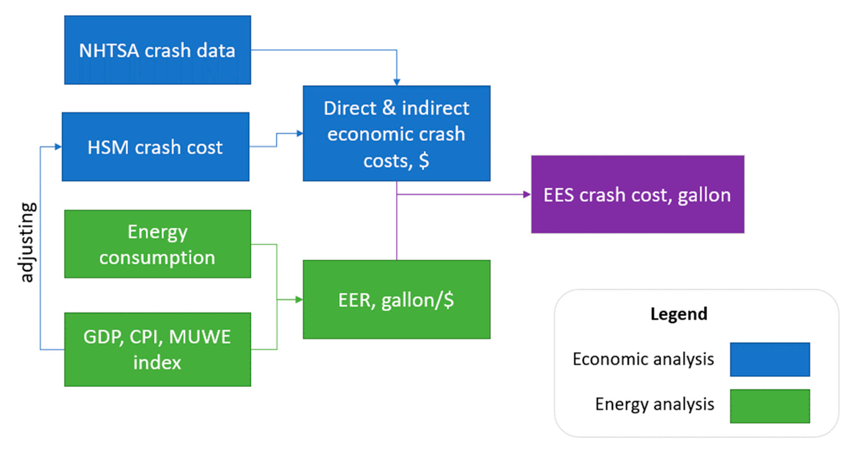
2.3. Energy Equivalence of Crash Cost

The conversion between the energy and monetary values was in part inspired by the embodied energy used in other disciplines, such as ecology, manufacturing, and construction. Embodied energy—defined as the available energy that has been used to make an ecosystem component, either directly or indirectly—has been used for the management of ecosystem services as well as natural resources accounting. It captures the “value” of the ecosystem elements that cannot be easily evaluated using traditional monetary valuation methodologies. In manufacturing, embodied energy is the total energy embodied by a manufactured product (e.g., automobiles, buildings) and processes used in its manufacturing, maintenance, and disposal [42,43]. As an example, a portion of the energy spent for the production workers (eating food, traveling to work, maintaining a lifestyle, etc.) is to be allocated to the embodied energy tally for a product [44].
In the food supply chain, a holistic view of the energy consumption concerning the upstream (production, transport, and processing) and downstream (distribution, transport, and consumption) aspects of food production was analyzed by referring to the embodied energy concept [45,46]. The energy consumption in the food supply chain is available in various data sets, including energy consumption for agriculture and aquaculture (Census of Agriculture [47]), food manufacturing (the Manufacturing Energy Consumption Survey [48] and the Annual Survey of Manufacturers [49]), transportation modes (Commodity Flow Survey [50]), food retail (Commercial Building Energy Consumption Survey [51]), and final consumption (Commercial Building Energy Consumption Survey [51]). To account for the embodied energy of the food supply chain, additional data sets were used for machinery, fertilizer, and pesticides (U.S. Department of Agriculture QuickStat [52]), and food nutritional energy (Food Balance Sheets [53]). In a similar fashion, this framework estimates embodied energy of the ecosystem (nationally) per unit of economic productivity, and then uses extensive economic impact studies to estimate the overall energy consequences of various types of crashes.
By the same token, the energy equivalence of crash cost comprises two parts: the direct energy cost and the indirect energy cost. The energy content of each is estimated using a gross domestic product to total national energy consumed ratio (as will be discussed later) to estimate total “embodied energy” of automotive crashes. Direct energy costs are estimated by the GDP-weighted energy equivalence of the direct economic costs. The indirect energy cost is converted from the indirect economic costs in the same manner. As with direct economic costs, several aspects of direct energy impacts are straightforward to estimate, with many precedents in the literature from which to draw. Many elements of the energy cost can be estimated in a straightforward manner, such as energy from induced congestion or energy from emergency response vehicles. However, other aspects are more difficult, such as rehabilitation activities or lost productivity of drivers due to induced congestion. The gross domestic product to total national energy consumed ratio is a convenient method to capture energy consequences if economic impacts are already known or estimated. The indirect energy cost is the energy equivalence of the cost that society is willing to pay to avoid the risk of injury and fatality crashes [21,28].

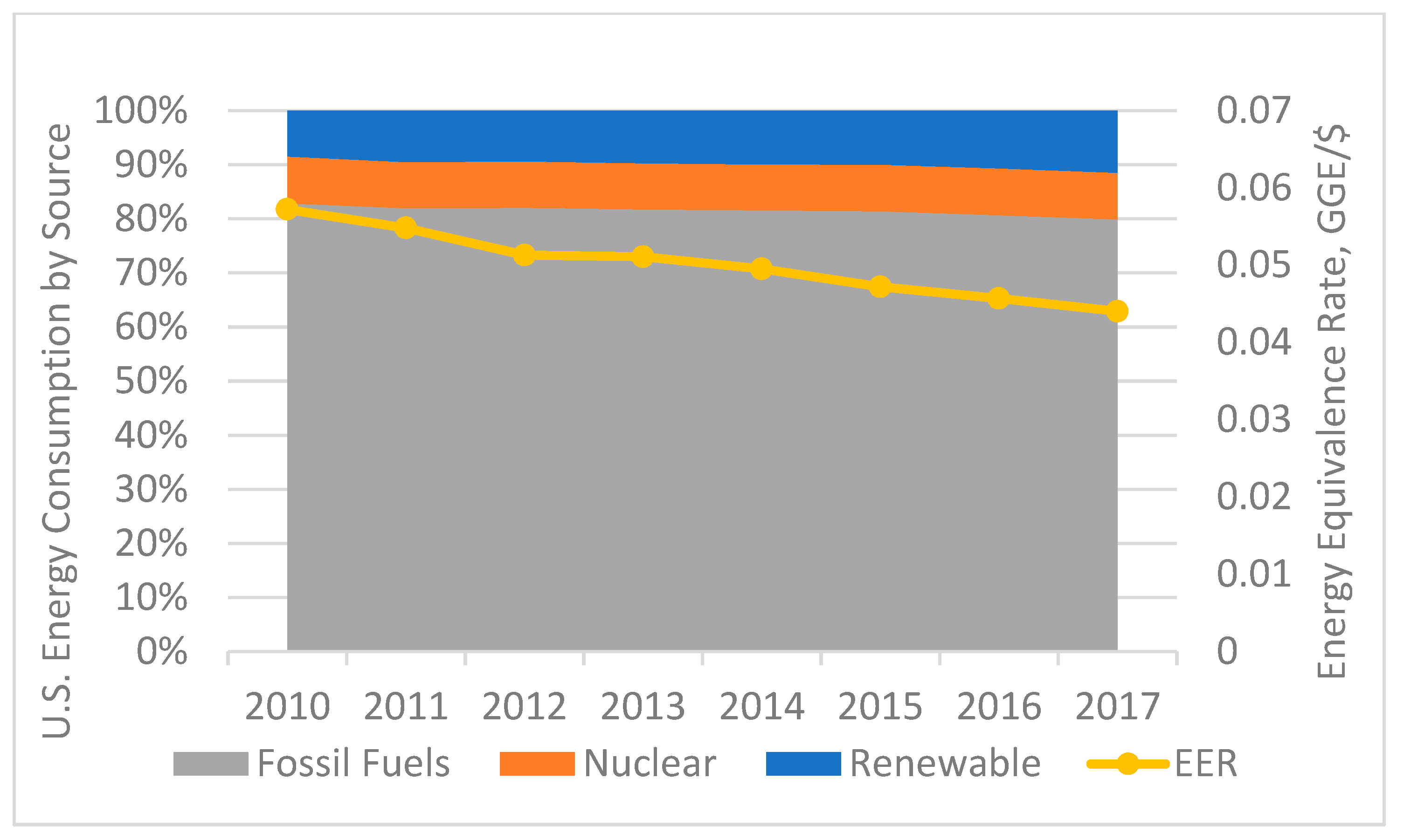
2.4. GDP-Weighted Energy Perspective

The energy consumption for all production sectors is estimated and expressed in British thermal units (BTUs) [54] by the Energy Information Administration (EIA). The energy consumption in BTU can also be converted to gasoline gallon equivalent (GGE), which represents the amount of energy contained in one gallon of gasoline. The GGE conversion factor is 114,000 BTU/GGE [55]. Using values of energy consumption and GDP of a specific year, the energy equivalence rate (EER) of the corresponding geographical area can be calculated. The higher the EER (expressed in BTU per dollar), the greater the amount of energy required to produce a unit value of GDP.
The framework hinges on an economic-to-energy-equivalence ratio in order to convert economic impacts to the equivalent energy impacts in terms of BTU or GGEs per crash type. The equivalency is determined at the national and state scale with estimated values of GDP (i.e., the value of all goods and services sold within the United States) and equivalent gross state product. If divided by population, the GPD can be apportioned on a per person basis. As of 2017, the GDP/person was USD 59,927, based on total GDP of USD 19.485 trillion dollars and a population of 325.7 million people [56]. (Note that this compares to a U.S. median income of USD 61,136 [57]).
On the energy side, the consumption of petroleum, natural gas, and coal (for electricity use) are the primary sources of energy accounted for in the method, constituting 80% of energy consumed in 2017 in the United States, as illustrated in Figure 3. Note that although solar, wind, nuclear, hydroelectric, geothermal, and other renewable/non-CO2-contributing sources of energy accounted for 20%, they are omitted in the methodology (as they are renewable or non-CO2 contributing), but they could be easily accounted for by factoring up appropriately [58]. In 2017, 36.2 quadrillion BTUs (36.2 quads) of petroleum, 28.0 quads of natural gas, and 13.9 quads of coal (based on BTU equivalents of each source) contributed to the total U.S. expenditure of energy supporting the total of USD 19.39 trillion GPD. Likewise, each of these can be apportioned (averaged) to individuals.
The primary theoretical argument in the framework is that economic impacts can be translated confidently to energy impacts by using the energy to GPD ratio as outlined above. Similar efforts to quantify broader impacts in the view of comprehensive resources used have been reported from various fields. Sima et al. [60] studied the energy intensity of labor for international trade in the European Union. In ecology, “emdollar” has been used as the economic equivalent of embodied energy, which is defined as the gross national product (GNP) equivalent to embodied energy contribution [61]. The embodied energy, defined as the available energy that is used directly or indirectly to make an ecosystem component, has been used for environmental accounting and decision making [62], such as for evaluating the natural capital for the U.S. National Forest System [63] and reforestation alternatives in Puerto Rico [64]. In construction, embodied energy is used to evaluate energy of production workers who eat food, travel to work, and maintain a lifestyle spending energy, part of which is allocated to their work [65,66]. Similar efforts can be done for quantifying the embodied energy in the operation, maintenance, and final demolition of the building.
When it comes to transportation, the economic impacts are not just vehicle efficiency or traffic dynamics efficiency (i.e., congestion). The larger impacts have to do with larger economic productivity aspects of the individual and the economy as a whole. Thus, in judging the broader, holistic impacts of crashes, we also have to take into account the energy intensity of the broad array of activities for which a crash impacts the economy. For example, in the case of a fatal crash, consider two impacts that can be measured economically but that are difficult to directly assert an energy measure. In a fatal crash, the deceased no longer contributes to the overall productivity of society. The investment in that person’s life in terms of resources to the point of their death is balanced against their productivity; that is, what each person invests back into society through their professional and personal lives.
Although a person’s worth cannot be wholly measured economically, economics is one area in which it can be measured and used as a mechanism to begin to understand energy consequences. A human begins to be highly economically productive after education and entering the workforce. All economic investment into the person can be considered an embedded or embodied resource. In the event of an untimely death, the investment of the embodied resources is lost, as well as the anticipated future productivity that the person would have contributed to society. Energy can be thought of in a similar fashion but is more difficult to quantify. Economics, however, through equivalencies described above, provides a surrogate method to estimate energy impacts related to embodied energy and its loss with respect to injury and death.
Similarly, “willingness to pay” is a concept in which economists assess the hazard premium that society as a whole puts on the value of risk associated with loss of life and injury. Similarly, this premium, which is based on VMR, has an energy equivalence in the broader term. Whether based on insurance premiums or the cost of increased safety features in cars (such as expensive anticollision features, crash safety design, or bigger/heavier vehicles to protect occupants), such willingness to pay has an economic impact that results in energy impacts (which are difficult to directly assess), which can be estimated by GDP-to-energy equivalencies.

3. Energy Equivalence of Safety Framework

The primary objective of the GDP-weighted energy equivalence of safety (EES) study is to estimate the energy impacts (measured in GGE) for various crash types. Figure 4 shows a flowchart for the EES calculation. The leftmost column outlines the primary data sources needed, which are (1) annual motor vehicle crash data from NHTSA, (2) HSM crash cost, (3) annual energy consumption from EIA, and (4) national economic statistics (e.g., GDP, CPI, MUWE index) from the Bureau of Transportation Statistics and the U.S. Department of Labor. The direct and indirect costs are adjusted temporally (year-to-year) by using CPI (Equation (2)) and MUWE (Equation (3)), respectively. The CPI measures the average change over time in the prices paid by urban consumers for a market basket of consumer goods and services [40]. MUWE indicates the real income growth that affects indirect cost. Both CPI and MUWE are available from the Department of Labor, and they vary over the years. The comprehensive cost of crashes is composed of indirect and direct costs, as shown in Equation (4). The energy equivalence rate (EER) for each year, defined by the methodology, is calculated by dividing energy consumption by GDP, as shown in Equation (5). The EER represents the marginal energy consumption of unit cost in GDP. Lastly, EES can be computed by multiplying the economic cost of crashes and corresponding EER (Equation (6)).
D i r e c t   c o s t 20 x x = D i r e c t   c o s t 2001   ×   C P I 20 x x C P I 2001
I n d i r e c t   c o s t 20 x x = I n d i r e c t   c o s t 2001   ×   M U W E 20 x x M U W E 2001
E c o n o m i c   c o s t   o f   s a f e t y   ( $ ) = D i r e c t   c o s t   ( $ ) + I n d i r e c t   c o s t   ( $ )
E E R   ( G G E / $ ) = E n e r g y   c o n s u m p t i o n G D P
E E S = E c o n o m i c   c o s t   o f   s a f e t y   ( $ ) * E E R   ( G G E / $ )

4. Energy Estimation Results Analysis

Using the proposed EES framework, motor vehicle crash analysis for national, state, and local levels across multiple years are presented in this section.

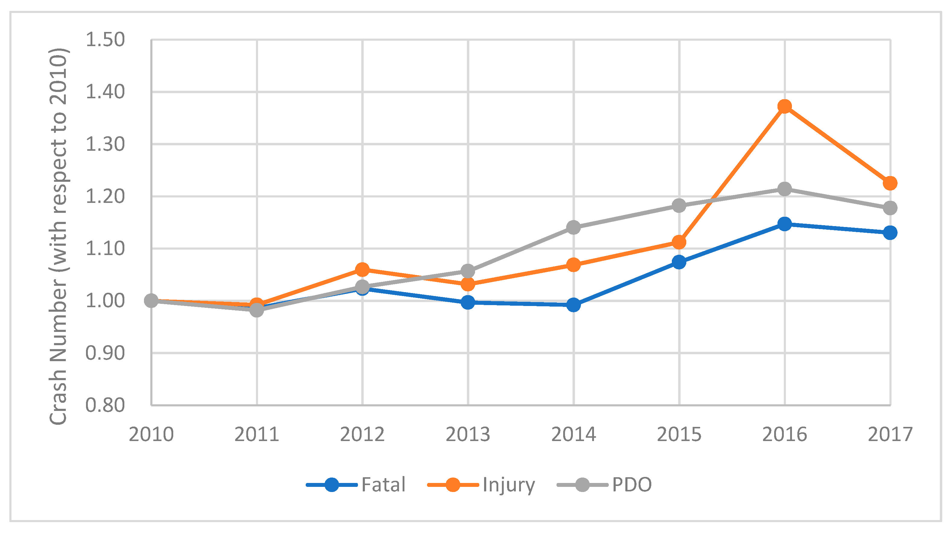
4.1. Crash Number and Economic Cost

Figure 5 shows the reported relative crash numbers (with respect to year 2010) from 2010 to 2017 for three crash types. The crash numbers of those are shown in Table 3. The changes of three crash types show a positive correlation (e.g., all with an increasing or decreasing trend) in most of the years and resembles the relationship in Heinrich’s Triangle [67], which represents a nearly fixed ratio of high-severity workplace accidents to lower-severity ones across multiple workplaces and suggests that reducing minor accidents would cause a proportional decrease in major accidents. With a smaller magnitude, the proportion of the fatal crash ranges from 0.50% to 0.56%. The injury crashes account for 27% to 31% of all crashes. The PDO crashes dominate the other two categories of crashes and account for 70% of total crashes. It is noticeable that the number of injury crashes spiked in 2016 and then dropped significantly in 2017. In 2016, a new sampling method implemented expanded the scope for injury crashes. This may contribute to the increase of injury crashes in 2016. NHTSA stressed that the 2016 and later year estimates are not comparable to 2015 and earlier year estimates [68]. However, we cannot rule out that the spike was solely because of the expanded scope—the actual injury crashes may have, in fact, increased in 2016.
The adjusted unit crash costs from 2010 to 2017 for all crash types are calculated according to Equations (1)–(3), and the costs are listed in Table 4. The increase in cost is attributed to the CPI and MUWE indexes that are closely related to the U.S. national economics. The unit crash cost value in 2001 from the HSM is used as the baseline for adjustment.

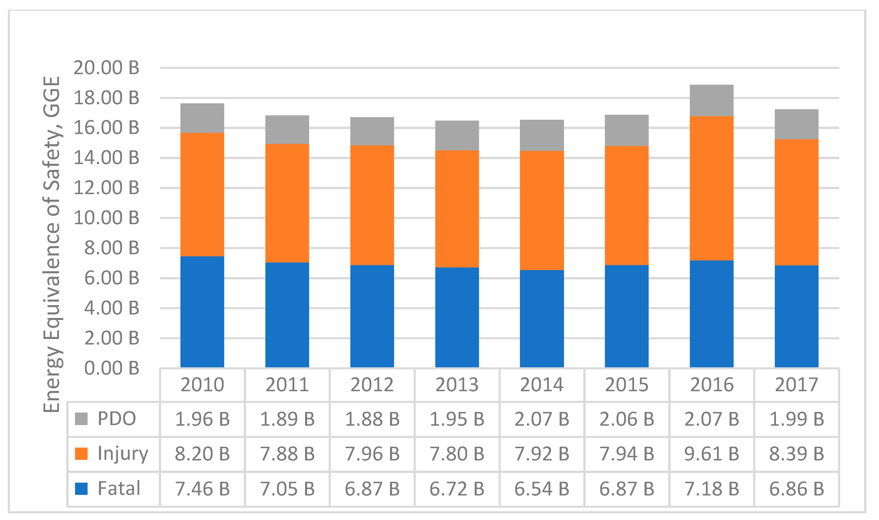
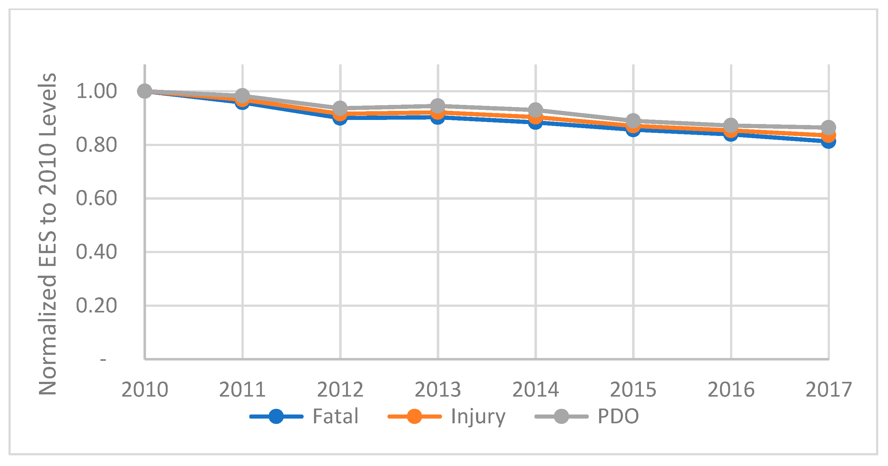
4.2. Gasoline Gallon Equivalent of Crash Cost

The U.S. national statistics for GDP as well as energy consumption for the analysis period (2010–2017) are shown in Table 5. The energy consumption is divided into three categories: renewable, nuclear, and fossil fuels. The percentage of energy source for fossil fuel decreased steadily from 2010 (82.8%) to 2017 (79.7%). On the other hand, the proportion of renewable energy sources, including geothermal, solar, wind, and biomass, increased to 11.4% in 2017 from the 8.5% observed in 2010. The percentage of nuclear energy remained at the same level. EER is calculated by Equation (4). The relative EERs with respect to the year 2010 are plotted in Figure 6. The EER exhibits a monotonically decreasing trend during the analysis period. According to the definition of EER, the declined trend indicates that energy productivity efficiency gets better over the years in the United States. In other words, GPD goes up while energy stays constant.
With the EER and unit crash cost, the energy equivalence of safety (EES) can be calculated using Equation (5) for multiple years, and the result is shown in Figure 7. The EES for fatal and injury crashes are of the same magnitude (ranging from 5 to 10 billion gallons), while the EES of PDO crashes is relatively small and about one-third of that of injury or fatal crashes. The total EES for fatal crashes was 17.62 billion GGE in 2010 and then declined to the lowest, 16.46 billion GGE, in 2013. It returned to 17.24 billion GGE in 2017. The total crash GGE experiences a similar trend as the fatal crash EES. The highest total EES was observed in 2016, at 18.86 billion GGE.
The EES per fatal and injury crashes were 246,360 and 5320 gallons, respectively. By contrast, the EES per PDO crash is only 508 gallons for the year 2010. The values of EES per crash for all crash types are illustrated in Table 6. The change of EES per crash for three crash types with regard to 2010 is displayed in Figure 8. The overall trend for EES per crash is declining, and it shares the same overall trend with the corresponding EER curve (shown in Figure 6). Compared to the economic factors such as CPI and MUWE, EER plays a more significant role in the value of EES.

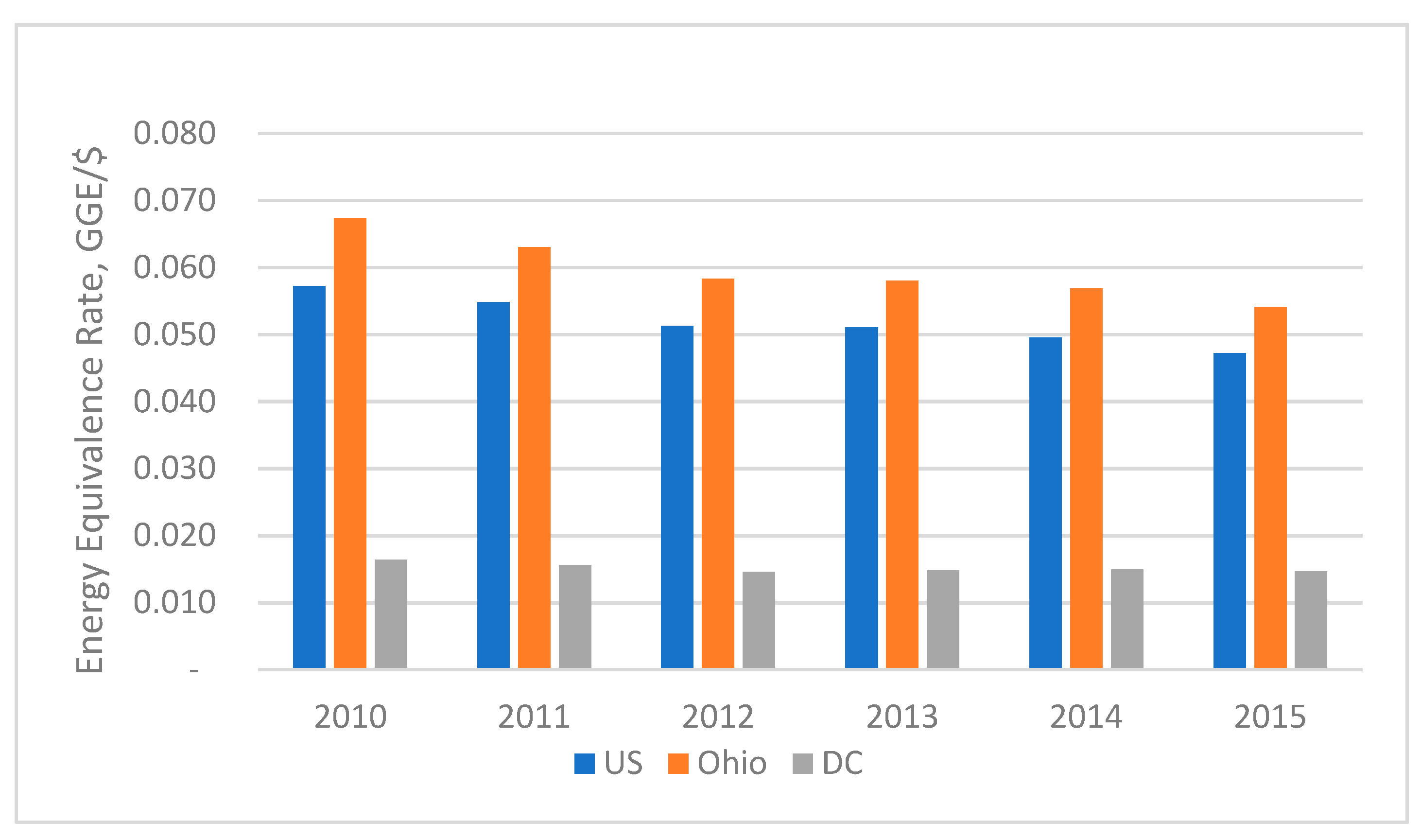
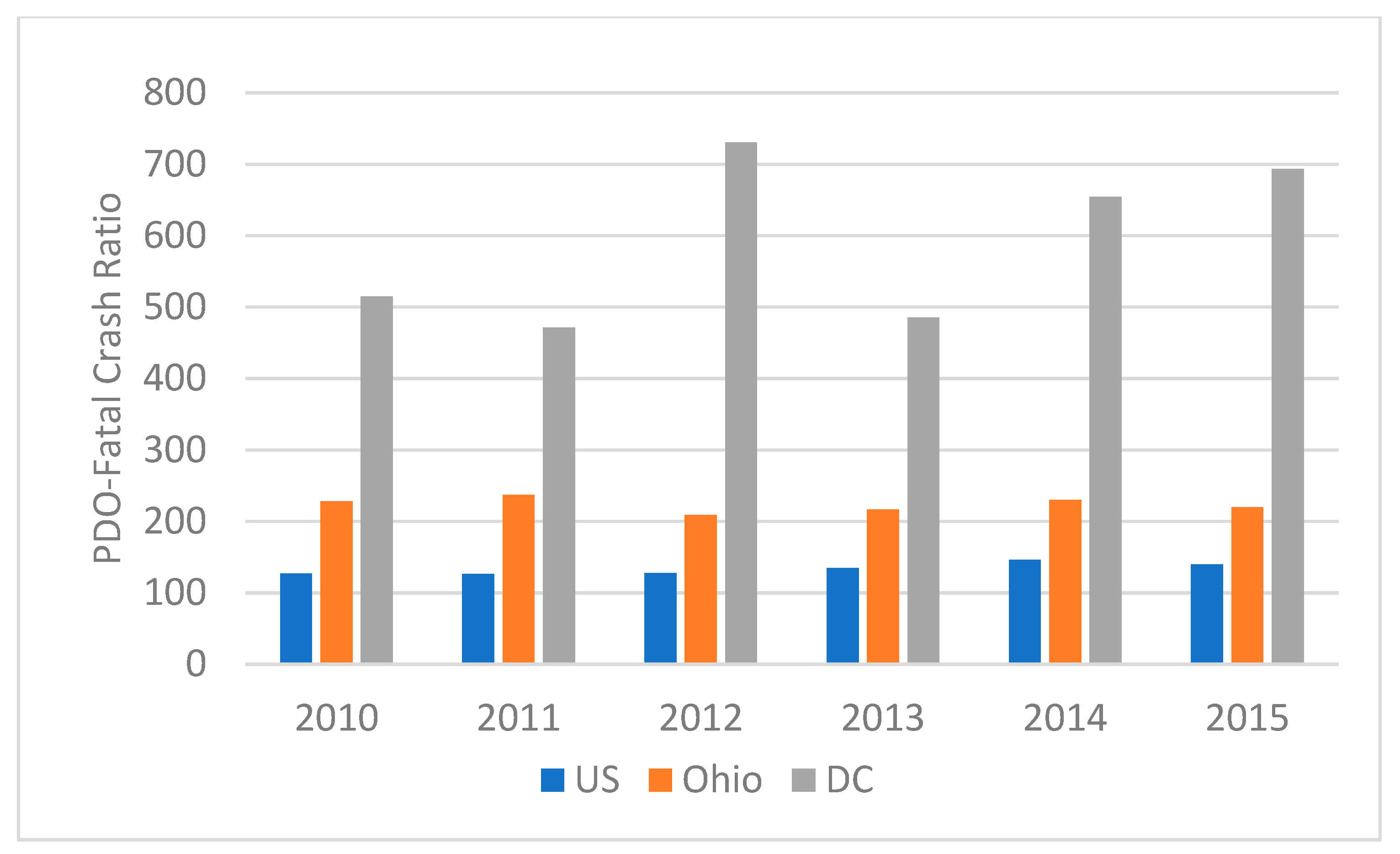
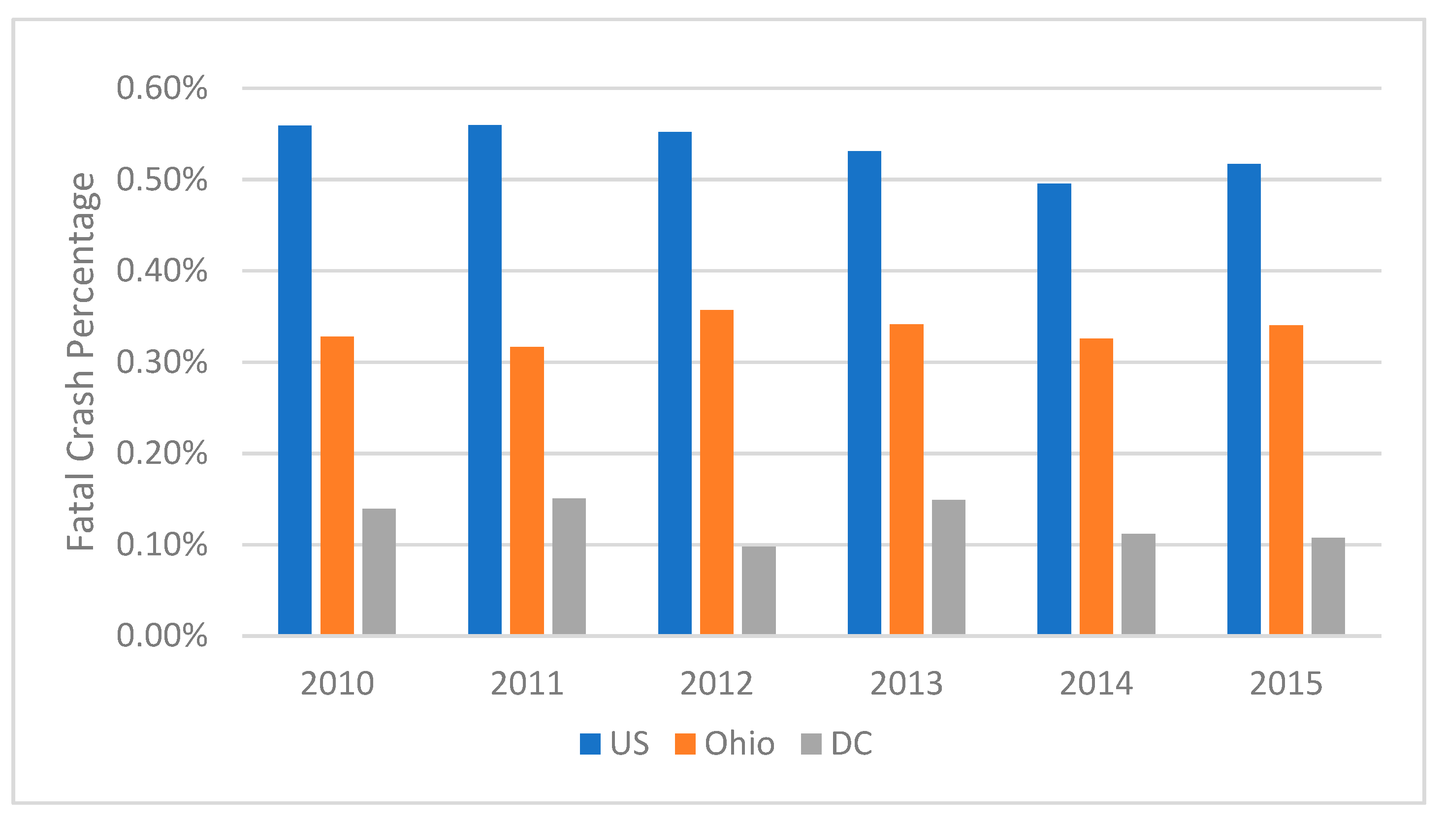
4.3. EES Analysis in Various Regional Scales

Besides national GDP-weighted EES, we compare the EES of both state and city levels and demonstrate the results in this section. The State of Ohio (state level) and Washington, D.C. (local level) are chosen for analysis. The results demonstrate the applicability of the framework to various regional levels. Due to the drastic difference in road users and transportation infrastructure (e.g., population, public road mileage), the crash number varies significantly across the national, state, and city levels. The EES per crash for Ohio and D.C. are shown in Table 7 and Table 8, respectively. The total number of crashes in Ohio is greater than that of D.C. The EES per crash also varies significantly between the two regions. On a per capita basis, the VMT for Ohio is nearly twice that of D.C.
To more closely examine the differences among the three regions, we calculate the energy consumption and GDP per capita and summarize it in Table 9. As shown, the difference between the United States and Ohio are marginal, but the differences with D.C. are significant. With respect to GDP per capita for all three regions, D.C. has the highest, which is more than three times that of Ohio and the national average. The high GDP per capita in D.C. greatly contributes to the low EER observed, with energy consumption for the three regions remaining at roughly the same level. The values of EER among the three regional scales are visualized in Figure 9. The low EER in D.C., which indicates higher energy productivity efficiency, is in part attributed to the composition of its economy. Nearly 30% of the employment in D.C. is from the government sector, and the service-producing industries (with government sector included) amount to almost 98% of the employment as of December 2017. The goods-producing sector (e.g., manufacturing), which is typical high energy intensity, only accounted for approximately 2% of the employment in D.C. [70]. As a typical state, Ohio’s EER pattern is close to the U.S. national-level EER pattern. Moreover, the energy consumption of D.C. exhibits an accelerated decreasing trend as compared to the rest of the US: the reduction in energy consumption per capita was 16% since 2010 in DC, compared to 4% at the national level and 3% in Ohio during the same five-year span.
Recall Heinrich’s Triangle, which represents the ratio among different accident severities. The ratio of fatal crashes to either injury or PDO crashes in D.C. is much lower than that for Ohio or even the United States, as shown in Figure 10. More specifically, for the occurrence of one fatal crash, the corresponding PDO crash is 693 for D.C. In comparison, the number for Ohio is 216 PDO crashes per fatal crash and the same number observed nationwide is 132 PDO crashes per fatal crash.
The percentage of fatal crashes among all crashes within each region is shown in Figure 11. Both Ohio and D.C. have a lower percentage of fatal crashes with respect to total crashes. D.C. has the lowest among the three, with 0.11% of the crashes classified as fatal crashes. The probability of fatal crashes for Ohio was also lower than the national average between 2010 and 2015.

5. Conclusions

This paper proposes a GDP-weighted approximation framework of the energy equivalence of safety that provides a holistic view for the long-term impacts on motor vehicle crashes with respect to energy consumption. The framework is used to analyze the energy impacts of motor vehicle crashes across multiple years (from 2010 to 2017). Previous attempts to estimate energy impacts of crashes were limited primarily to induced congestion and resulting wasted fuel. Based on national congestion studies, the amount of wasted fuel from all crashes was slightly less than 500 gallons per crash (across all types of crashes, including fatal, injury, and PDO) in 2015. The methods presented here entailed taking an embodied energy framework, estimating the energy impact of each type of crash resulting from both direct and indirect consequences, leveraging extensive economic impact studies and a GDP-to-national-energy-consumption ratio to estimate the ecosystem-dependent holistic energy impact. This resulted in per crash energy estimates of 200,259, 4442, and 439 GGE for fatal, injury, and property-damage-only crashes, respectively. Factoring the total number of crashes in each category (for 2017), the total estimated per crash energy impact is 2679 GGE, or over five times higher than the previous estimate.
The analysis of EES across multiple years shows that the EES for the United States decreased from 17.62 million GGE in 2010 to 16.47 million GGE in 2013. It then started to rise and reached 18.86 million GGE in 2016. Despite this fluctuation, the magnitude of total EES is relatively constant. In addition, the energy equivalence rate (EER) across the three crash types experienced a steady decline nationwide over the analysis period. By 2017, the EER (200,000 GGE) was 81% of that in 2010 for a fatal crash, due to the increased energy efficiency of the overall U.S. economy. Besides the national-level analysis, we also conducted EES analyses at the state and city level across multiple years to demonstrate the framework’s applicability. The analysis revealed that the composition of the economy plays an important role in determining the EES values for a geographic region, and that crash ratios between fatal, injury, and property damage only vary significantly.

Author Contributions

Conceptualization, S.Y. L.Z. and Z.Z.; data curation and visualization, Z.Z.; analysis and investigation, Z.Z., S.Y. and L.Z.; writing—original draft preparation, Z.Z.; writing—review and editing, L.Z. and S.Y.; supervision, S.Y. All authors have read and agreed to the published version of the manuscript.

Funding

This research was funded by U.S. DOE Vehicle Technologies Office (VTO) under the Systems and Modeling for Accelerated Research in Transportation (SMART) Mobility Laboratory Consortium, an initiative of the Energy Efficient Mobility Systems (EEMS) Program and The APC was funded by SMART Mobility Laboratory Consortium project.

Acknowledgments

This work was authored by the National Renewable Energy Laboratory, operated by Alliance for Sustainable Energy, LLC, for the U.S. Department of Energy (DOE) under Contract No. DE-AC36-08GO28308. Funding was provided by the DOE Vehicle Technologies Office (VTO) under the Systems and Modeling for Accelerated Research in Transportation (SMART) Mobility Laboratory Consortium, an initiative of the Energy Efficient Mobility Systems (EEMS) Program. The views expressed in the article do not necessarily represent the views of the DOE or the U.S. Government. The U.S. Government retains and the publisher, by accepting the article for publication, acknowledges that the U.S. Government retains a nonexclusive, paid-up, irrevocable, worldwide license to publish or reproduce the published form of this work, or allow others to do so, for U.S. Government purposes.

Conflicts of Interest

The authors declare no conflict of interest.

Abbreviations

AASHTOAmerican Association of State Highway Transportation Officials
AISAbbreviated Injury Scale
BtuBritish thermal unit
CDSCrashworthiness Database System
CISSCrash Investigation Sampling System
CPIConsumer Price Index
CRSSCrash Report Sampling System
EERenergy equivalence rate
EESenergy equivalence of safety
EIAEnergy Information Administration
EPAU.S. Environmental Protection Agency
EPDOequivalent property damage only
GDPgross domestic product
GESGeneral Estimate System
GGEgasoline gallon equivalent
HSMHighway Safety Manual
MAISMaximum Abbreviated Injury Scale
MOVESMulti-scale mOtor Vehicle and equipment Emission System
MUWEmedian usual weekly earnings
NHTSANational Highway Transportation Safety Administration
PDOproperty damage only
QALYquality-adjusted life years
quadquadrillion (1015) Btu
VMRvalue of mortality risk
VMTvehicle miles traveled
VSLvalue of a statistical life

References

  1. Papadoulis, A.; Quddus, M.; Imprialou, M.-I.M. Evaluating the safety impact of connected and autonomous vehicles on motorways. Accid. Anal. Prev. 2019, 124, 12–22. [Google Scholar] [CrossRef] [PubMed] [Green Version]
  2. Virdi, N.; Grzybowska, H.; Waller, S.T.; Dixit, V.V. A safety assessment of mixed fleets with Connected and Autonomous Vehicles using the Surrogate Safety Assessment Module. Accid. Anal. Prev. 2019, 131, 95–111. [Google Scholar] [CrossRef] [PubMed]
  3. Martin-Gasulla, M.; Sukennik, P.; Lohmiller, J. Investigation of the Impact on Throughput of Connected Autonomous Vehicles with Headway Based on the Leading Vehicle Type. Transp. Res. Rec. J. Transp. Res. Board 2019, 2673, 617–626. [Google Scholar] [CrossRef]
  4. Gettman, D.; Head, K.L. Surrogate Safety Measures from Traffic Simulation Models. Transp. Res. Rec. J. Transp. Res. Board 2003, 1840, 104–115. [Google Scholar] [CrossRef] [Green Version]
  5. National Highway Traffic Safety Administration. Traffic Safety Facts Annual Report 2019. Available online: https://cdan.nhtsa.gov/tsftables/tsfar.htm (accessed on 4 May 2020).
  6. De Leur, P.; Eng, P.; Thue, L.; Ladd, M.B. Capital Region Intersection Safety Partnership. Available online: https://drivetolive.ca/blog/2018/06/15/updated-cost-of-collision-study/ (accessed on 10 July 2010).
  7. Zhu, L.; Young, S.E.; Day, C.M. Exploring First-Order Approximation of Energy Equivalence of Safety at Intersections; National Renewable Energy Lab.(NREL): Golden, CO, USA, 2019. [Google Scholar]
  8. Ogden, K.W. Safer Roads: A Guide to Road Safety Engineering; Ashgate: Aldershot, UK, 1996. [Google Scholar]
  9. Mannering, F.L.; Shankar, V.N.; Bhat, C.R. Unobserved heterogeneity and the statistical analysis of highway accident data. Anal. Methods Accid. Res. 2016, 11, 1–16. [Google Scholar] [CrossRef]
  10. Sobhani, A.; Young, W.; Logan, D.; Bahrololoom, S. A kinetic energy model of two-vehicle crash injury severity. Accid. Anal. Prev. 2011, 43, 741–754. [Google Scholar] [CrossRef]
  11. Schmidová, N.; Zavřelová, T.; Vašíček, M.; Zavadil, F.; Růžička, M.; Rund, M. Development of Adaptable CFRP Energy Absorbers for Car Crashes. Mater. Today Proc. 2018, 5, 26784–26791. [Google Scholar] [CrossRef]
  12. Zhang, X.; Jin, X.; Li, Y.; Li, G. Improved design of the main energy-absorbing automotive parts based on traffic accident analysis. Mater. Des. 2008, 29, 403–410. [Google Scholar] [CrossRef]
  13. Reddy, T.; Narayanamurthy, V.; Rao, Y. Evolution of a new geometric profile for an ideal tube inversion for crash energy absorption. Int. J. Mech. Sci. 2019, 155, 125–142. [Google Scholar] [CrossRef]
  14. Sivasaravanan, S.; Raja, V.B.; Kumar, P.S.; Vardhan, V.H. Fabrication of Porous Composite Material for Crash Energy Absorption. Mater. Today Proc. 2019, 16, 972–977. [Google Scholar] [CrossRef]
  15. Kaczyński, P.; Gronostajski, Z.; Polak, S. Progressive crushing as a new mechanism of energy absorption. The crushing study of magnesium alloy crash-boxes. Int. J. Impact Eng. 2019, 124, 1–8. [Google Scholar] [CrossRef]
  16. Chung, Y.; Recker, W.W. Spatiotemporal Analysis of Traffic Congestion Caused by Rubbernecking at Freeway Accidents. IEEE Trans. Intell. Transp. Syst. 2013, 14, 1416–1422. [Google Scholar] [CrossRef]
  17. Eisele, W.L.; Schrank, D.L.; Bittner, J.; Larson, G. Incorporating Urban-Area Truck Freight Value into the Urban Mobility Report. Transp. Res. Rec. J. Transp. Res. Board 2013, 2378, 54–64. [Google Scholar] [CrossRef]
  18. Koupal, J.; Cumberworth, M.; Michaels, H.; Beardsley, M.; Brzezinski, D. Design and implementation of MOVES: EPA’s new generation mobile source emission model. Ann Arbor 2003, 1001, 105. [Google Scholar]
  19. Rakha, H.A.; Ahn, K.; Trani, A. Development of VT-Micro model for estimating hot stabilized light duty vehicle and truck emissions. Transp. Res. Part D Transp. Environ. 2004, 9, 49–74. [Google Scholar] [CrossRef]
  20. Brooker, A.; Gonder, J.; Wang, L.; Wood, E.; Lopp, S.; Ramroth, L. FASTSim: A Model to Estimate Vehicle Efficiency, Cost and Performance. SAE Tech. Pap. Ser. 2015, 1. Available online: https://saemobilus.sae.org/content/2015-01-0973/ (accessed on 8 May 2020).
  21. Blincoe, L.; Miller, T.R.; Zaloshnja, E.; Lawrence, B.A. The Economic and Societal Impact of Motor Vehicle Crashes, 2010 (Revised); National Highway TrafficSafety Administration: Washington, DC, USA, 2015.
  22. Radja, G.A. National Automotive Sampling System–Crashworthiness Data System, 2015 Analytical User’s Manual; National Highway TrafficSafety Administration: Washington, DC, USA, 2016.
  23. National Highway Traffic Safety Administration. NASS General Estimates System. 2019. Available online: https://www.nhtsa.gov/national-automotive-sampling-system-nass/nass-general-estimates-system (accessed on 8 May 2020).
  24. National Highway Traffic Safety Administration. Crashworthiness Data System. 2019. Available online: https://www.nhtsa.gov/national-automotive-sampling-system-nass/crashworthiness-data-system (accessed on 9 May 2020).
  25. National Highway Traffic Safety Administration. Crash Report Sampling System (CRSS). 2019. Available online: https://www.nhtsa.gov/crash-data-systems/crash-report-sampling-system-crss (accessed on 8 May 2020).
  26. National Highway Traffic Safety Administration. Crash Investigation Sampling System (CISS). 2019. Available online: https://www.nhtsa.gov/crash-data-systems/crash-investigation-sampling-system (accessed on 8 May 2020).
  27. Chen, C.-L.; Subramanian, R.; Zhang, F.; Noh, E.Y. NHTSA’s Data Modernization Project. In Proceedings of the 2015 Federal Committee on Statistical Methodology (FCSM) Research Conference, Washington, DC, USA, 1–3 December 2015. [Google Scholar]
  28. Harmon, T.; Bahar, G.; Gross, F. Crash Costs for Highway Safety Analysis; Federal Highway Administration: McLean, VA, USA, 2018.
  29. Najm, W.G.; Smith, J.D.; Yanagisawa, M. Pre-crash Scenario Typology for Crash Avoidance Research. In DOT HS; National Highway TrafficSafety Administration: Washington, DC, USA, 2007. [Google Scholar]
  30. Silcock, R. Guidelines for estimating the cost of road crashes in developing countries. Lond. Dep. Int. Dev. Proj. 2003, 7780, 2003. [Google Scholar]
  31. American Association of State Highway and Transportation Officials. Highway Safety Manual; American Association of State Highway Transportation Officials (AASHTO): Washington, DC, USA, 2010.
  32. Viscusi, W.K.; Aldy, J. The value of a statistical life: A critical review of market estimates throughout the world. J. Risk Uncertain. 2003, 27, 5–76. [Google Scholar] [CrossRef]
  33. Machina, M.; Viscusi, W.K. Handbook of the Economics of Risk and Uncertainty; Newnes: Oxford, UK, 2013. [Google Scholar]
  34. Cameron, T.A. Euthanizing the value of a statistical life. Rev. Environ. Econ. Policy 2010, 4, 161–178. [Google Scholar] [CrossRef] [Green Version]
  35. Robinson, L.A.; Hammitt, J.K. Research Synthesis and the Value per Statistical Life. Risk Anal. 2015, 35, 1086–1100. [Google Scholar] [CrossRef]
  36. Elias, B. Screening and Securing Air Cargo: Background and Issues for Congress; Congressional Research Service: Washington, DC, USA, 2010.
  37. Transportation Safety Administration. Air Cargo Screening Final Rule; United States Office of the Federal Register: Washington, DC, USA, 2011.
  38. Kniesner, T.J.; Viscusi, W.K. The value of a statistical life. Oxford Res. Encycl. Econ. Financ. 2019. Available online: https://papers.ssrn.com/sol3/papers.cfm?abstract_id=3379967#:~:text=The%20value%20of%20a%20statistical%20life%20(VSL)%20is%20the%20local,marginal%20cost%20of%20enhancing%20safety (accessed on 13 August 2020).
  39. Bosworth, R.; Hunter, A.; Kibria, A.; STRATA. The Value of a Statistical Life: Economics and Politics; STRATA: Logan, UT, USA, 2017. [Google Scholar]
  40. Bryan, M.; Cecchetti, S. The Consumer Price Index as a Measure of Inflation; National Bureau of Economic Research: Cambridge, MA, USA, 1993.
  41. Moran, M.J.; Monje, C. Guidance of Treatment of the Economic Value of a Statistical Life in U.S. Department of Transportation Analyses-2016 Adjustment; US Department of Transportation: Washington, DC, USA, 2016.
  42. Stephan, A.; Stephan, L. Reducing the total life cycle energy demand of recent residential buildings in Lebanon. Energy 2014, 74, 618–637. [Google Scholar] [CrossRef] [Green Version]
  43. Rauf, A.; Crawford, R.H. The Effect of Material Service Life on the Life Cycle Energy of Residential Buildings. In Proceedings of the ASA2012: The 46th Annual Conference of the Architectural Science Association (formerly ANZAScA)–Building on Knowledge: Theory and Practice, Queensland, Australia, 14–16 November 2012. [Google Scholar]
  44. Dixit, M.K. Life cycle recurrent embodied energy calculation of buildings: A review. J. Clean. Prod. 2019, 209, 731–754. [Google Scholar] [CrossRef]
  45. Pagani, M.; De Menna, F.; Johnson, T.G.; Vittuari, M. Impacts and costs of embodied and nutritional energy of food losses in the US food system: Farming and processing (Part A). J. Clean. Prod. 2020, 244, 118730. [Google Scholar] [CrossRef]
  46. Vittuari, M.; Pagani, M.; Johnson, T.G.; De Menna, F. Impacts and costs of embodied and nutritional energy of food waste in the US food system: Distribution and consumption (Part B). J. Clean. Prod. 2020, 252, 119857. [Google Scholar] [CrossRef]
  47. National Agricultural Statistics Service. Census of Agriculture; U.S. Department of Agriculture: Washington, DC, USA, 2012. Available online: https://www.nass.usda.gov/AgCensus/index.php (accessed on 13 May 2020).
  48. U.S. Energy Information Administration. Manufacturing Energy Consumption Survey Data. 2017. Available online: https://www.eia.gov/consumption/data.php#mfg (accessed on 13 May 2020).
  49. U.S. Census Bureau. Annual Survey of Manufacturers. Available online: https://www.census.gov/econ/overview/ma0300.html (accessed on 8 May 2020).
  50. The Bureau of Transportation Statistics. Commodity Flow Survey Overview. 2017. Available online: https://www.bts.gov/cfs (accessed on 13 May 2020).
  51. File, M. Commercial Buildings Energy Consumption Survey (CBECS); US Department of Energy: Washington, DC, USA, 2015.
  52. United States Department of Agriculture. QuickStats. 2020. Available online: https://quickstats.nass.usda.gov/ (accessed on 13 May 2020).
  53. FAOSTAT. Food and Agriculture Organization of the United Nations, Statistics Division. Forestry Production and Trade. Available online: http://www.fao.org/faostat/en/#data/FO (accessed on 4 April 2019).
  54. Energy Information Administration. Annual Energy Outlook; Energy Information Administration, U.S. Department of Energy: Washington, DC, USA, 2010.
  55. Department of Energy. Gasoline and Diesel Gallon Equivalency Methodology. Available online: https://afdc.energy.gov/fuels/equivalency_methodology.html (accessed on 13 May 2020).
  56. The World Bank. GDP Per Capita-United States. 2020. Available online: https://data.worldbank.org/indicator/NY.GDP.PCAP.CD?locations=US (accessed on 12 May 2020).
  57. Federal Reserve Economic Data. Median Household Income in the United States. 2020. Available online: https://fred.stlouisfed.org/series/MEHOINUSA646N (accessed on 11 May 2020).
  58. U.S. Energy Infomration Administration. Annual Energy Review. Available online: https://www.eia.gov/totalenergy/data/annual/ (accessed on 12 August 2020).
  59. Energy Infomation Administration. Energy information administration. Dep. Energy 2010, 92010, 1–15. [Google Scholar]
  60. Simas, M.; Wood, R.; Hertwich, E. Labor embodied in trade: The role of labor and energy productivity and implications for greenhouse gas emissions. J. Ind. Ecol. 2015, 19, 343–356. [Google Scholar] [CrossRef]
  61. Odum, H.T.; Odum, E.P. The Energetic Basis for Valuation of Ecosystem Services. Ecosyststems 2000, 3, 21–23. [Google Scholar] [CrossRef]
  62. Odum, H.T. Environmental Accounting: Energy and Environmental Decision Making; Wiley: New York, NY, USA, 1996; Volume 707. [Google Scholar]
  63. Campbell, E.; Brown, M.T. Environmental accounting of natural capital and ecosystem services for the US National Forest System. Environ. Dev. Sustain. 2012, 14, 691–724. [Google Scholar] [CrossRef]
  64. Odum, H.T.; Doherty, S.J.; Scatena, F.N.; Kharecha, P.A. Energy Evaluation of Reforestation Alternatives in Puerto Rico. For. Sci. 2000, 46, 521–530. [Google Scholar]
  65. Dixit, M.K. Embodied Energy Calculation: Method and Guidelines for a Building and Its Constituent Materials. Ph.D. Thesis, Texas A&M University, College Station, TX, USA, 15 December 2013. [Google Scholar]
  66. Jiao, Y.; Lloyd, C.; Wakes, S.J. The relationship between total embodied energy and cost of commercial buildings. Energy Build. 2012, 52, 20–27. [Google Scholar] [CrossRef]
  67. Bin-Nun, A.Y.; Panasci, A.; Tebbens, R.J.D. Heinrich’s Triangle, Heavy-Tailed Distributions, and Autonomous Vehicle Safety. In Proceedings of the 99th Transportation Research Board Annual Meeting, Washington, DC, USA, 12–16 January 2020. [Google Scholar]
  68. National Highway Traffic Safety Administration. Traffic Safety Facts 2017; National Highway Traffic Safety Administration: Washington, DC, USA, 2019.
  69. U.S. Census Bureau. Population and Housing Unit Estimates Datasets. 2019. Available online: https://www.census.gov/programs-surveys/popest/data/data-sets.html (accessed on 8 June 2020).
  70. D.C. Department of Employment Services, District of Columbia. Wage and Salary Employment by Industry and Place of Work; US Bureau of Labour Statistics: Washington, DC, USA, 2017.
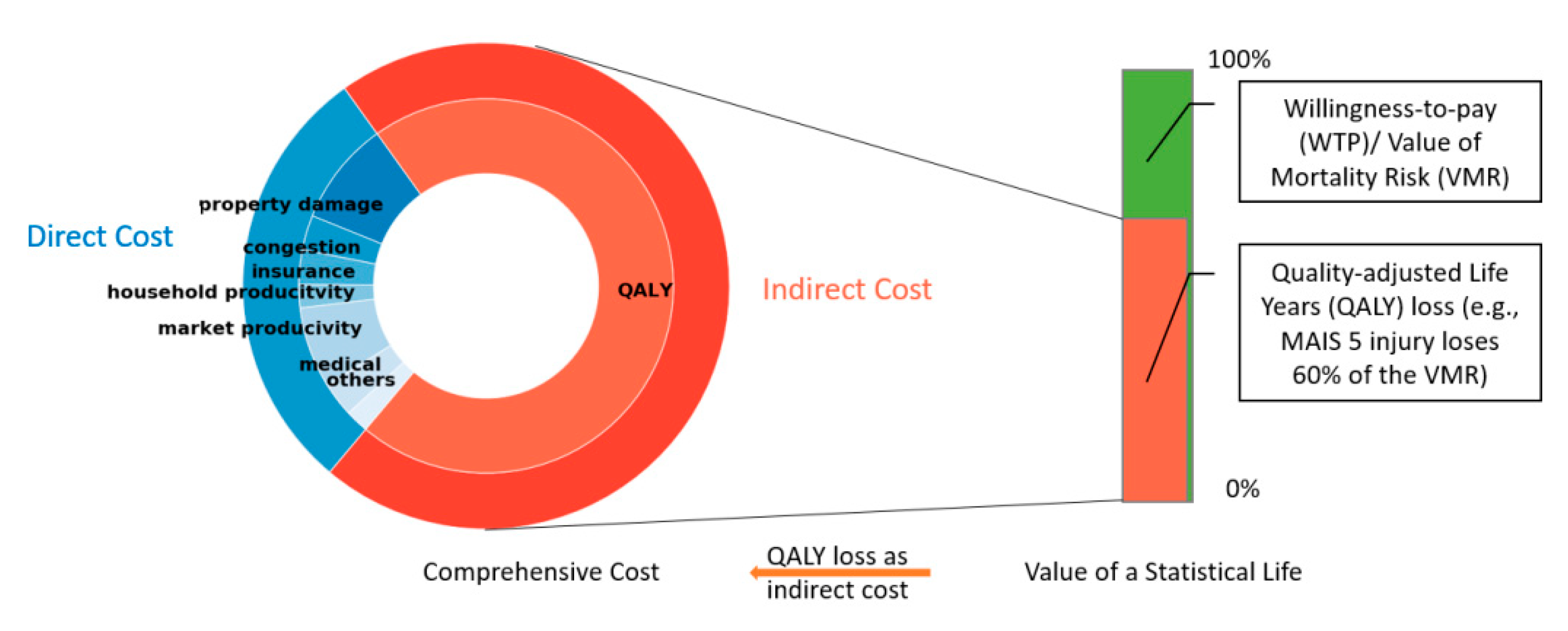
Figure 1. Cost composition and relationship. Note: quality-adjusted life year, QALY; willingness-to-pay, WTP; value of mortality risk, VMR.
Energies 13 04230 g001
Figure 2. Value of mortality risk (VMR) example: Air Cargo Screening analysis.
Energies 13 04230 g002
Figure 3. U.S. primary energy consumption by source and sector, 2017 [59].
Energies 13 04230 g003
Figure 4. Energy equivalence flowchart. Note: NHTSA, National Highway Traffic Safety Administration; HSM, Highway Safety Manual; CPI, Consumer Price Index; MUWE, median usual weekly earnings; EER, energy equivalence rate; EES, energy equivalence of safety.
Energies 13 04230 g004
Figure 5. Relative crash number (with respect to 2010).
Energies 13 04230 g005
Figure 6. Change of energy equivalence rate (EER).
Energies 13 04230 g006
Figure 7. Total gasoline gallon equivalent (GGE) cost from 2010 to 2017.
Energies 13 04230 g007
Figure 8. Change of EES per crash.
Energies 13 04230 g008
Figure 9. Comparison of energy equivalence rate for the United States, Ohio, and Washington, D.C.
Energies 13 04230 g009
Figure 10. Crash severity relationship: Heinrich’s Triangle.
Energies 13 04230 g010
Figure 11. Crash severity relationship: fatal crash percentage.
Energies 13 04230 g011
Table 1. Crash cost classification by HSM.
Cost CategoryCost Item
Direct costsMedical costs
Emergency medical services
Lost productivity (short-term)
Workplace losses
Insurance administration costs
Legal and court expenses
Congestion costs
Property damage costs
Human capital cost (long-term)
Indirect cost (monetized pain and suffering)Quality-adjusted life year
Table 2. Crash unit cost in 2001 U.S. dollars (Source: Highway Safety Manual [31]).
Crash Severity
(KABCO Scale)
Direct Unit Cost a
(Economic Crash Unit Cost)
Indirect Unit Cost
(QALY Crash Unit Cost)
Comprehensive Unit CostEPDO
Fatality (K)$1,245,600$2,763,300$4,008,900542
Injury (A/B/C)$44,268$38,332$82,60011
PDO (O)$6400$1000$74001
a All values in the table are obtained from the Highway Safety Manual. Note: PDO, property damage only; EPDO, equivalent property damage only.
Table 3. Annual crash numbers and ratios of three crash types.
YearFatalInjuryPDOTotal
201030,2960.56%1,542,00028%3,847,00071%5,419,296
201129,8760.56%1,530,00029%3,778,00071%5,337,876
201231,0060.55%1,634,00029%3,950,00070%5,615,006
201330,2020.53%1,591,00028%4,066,00071%5,687,202
201430,0560.50%1,648,00027%4,387,00072%6,065,056
201532,5390.52%1,715,00027%4,548,00072%6,295,539
201634,7480.51%2,116,00031%4,670,00068%6,820,748
201734,2470.53%1,889,00029%4,530,00070%6,453,247
Table 4. Adjusted unit crash cost (USD) of three types.
YearFatalInjuryPDO
2010$4,305,731$92,973$8886
2011$4,305,139$94,009$9116
2012$4,321,692$94,949$9279
2013$4,353,499$95,903$9403
2014$4,396,230$97,070$9545
2015$4,471,366$98,155$9582
2016$4,525,052$99,359$9703
2017$4,548,077$100,882$9976
Table 5. National GDP (USD) and energy consumption statistics.
YearGDP
(Trillion $)
Renewable Consumption PercentageNuclear Consumption PercentageFossil Fuels Consumption PercentageEnergy Consumption (Quads)EER (Btu/$)
201015.08.5%8.6%82.8%97.66523
201115.59.5%8.5%81.8%97.06248
201216.29.4%8.5%81.9%94.55848
201316.79.7%8.5%81.6%97.25824
201417.49.9%8.5%81.4%98.45645
201518.110.0%8.6%81.2%97.55380
201618.710.6%8.7%80.5%97.45209
201719.511.4%8.6%79.7%97.85020
Source: Annual Energy Review [58].
Table 6. Energy equivalence of safety (EES) per crash type.
CategoryFatal (GGE)Injury (GGE)PDO (GGE)
YearDirectIndirectTotalDirectIndirectTotalDirectIndirectTotal
201076,544169,816246,36028732447532043969508
201173,306162,632235,93827822370515243368501
201268,883152,820221,70326302241487141264476
201369,108153,319222,42726462254490041565480
201467,638150,059217,69725962211480740964473
201565,560145,446211,00625012131463239161452
201664,241142,521206,76224522088454038360443
201762,220138,039200,25923992043444238059439
Table 7. EES analysis for the State of Ohio.
YearPopulation [69]Crash NumberEES per Crash (GGE)
FatalInjuryPDOFatalInjuryPDO
201011,539,33698474,426224,750289,9696261598
201111,544,66394273,771223,118271,3765926575
201211,548,923102472,105213,956252,0375537541
201311,576,68491869,104199,056252,5585564546
201411,602,70091969,917211,532249,9875520543
201511,617,527102975,107226,169241,9125310518
Table 8. EES analysis for Washington, D.C.
YearPopulationCrash NumberEES per Crash (GGE)
FatalInjuryPDOFatalInjuryPDO
2010605,22625506012,87070,6941526146
2011619,80027521012,71466,9811463142
2012634,92418525813,15263,1551388136
2013650,58129535814,06964,4621420139
2014662,32824581115,70465,8171453143
2015675,40026621518,02465,5821440141
Table 9. Ohio and D.C. comparison, per capita basis.
YearEnergy Consumption (GGE) per CapitaGDP (USD) per Capita
USOhioDCUSOhioDC
201027482912275948,03143,242168,018
201127102886259949,44745,785167,052
201226232779238851,12547,649163,379
201326792830235752,43948,778159,150
201426922899237454,35350,978158,595
201526482828231856,11152,277158,043

