Abstract
A modified particle swarm optimization and incorporated chaotic search to solve economic dispatch problems for smooth and non-smooth cost functions, considering prohibited operating zones and valve-point effects is proposed in this paper. An inertia weight modification of particle swarm optimization is introduced to enhance algorithm performance and generate optimal solutions with stable solution accuracy and offers faster convergence characteristic. Moreover, an incorporation of chaotic search, called logistic map, is used to increase the global searching capability. To demonstrate the effectiveness and feasibility of the proposed algorithm compared to the several existing methods in the literature, five systems with different criteria are verified. The results show the excellent performance of the proposed method to solve economic dispatch problems.
1. Introduction
In electric power systems, an economic dispatch (ED) problem is a basic optimization problem, with the main aim to reduce the total cost of the power generation operation. Basically, all solutions to solving ED problems in [1,2,3,4,5,6] can be split into: (1) traditional optimization methods and (2) evolutionary computation-based optimization techniques. ED problems can be solved by several mathematical programming methods, such as lambda iteration, base point, and participation factor method [1], interior point method [2], and with evolutionary computation-based optimization techniques, such as artificial neural networks [3]. The ED problems, with smooth and non-smooth functions, were performed in previous years by taking into consideration generation constraints, such as valve-point effects (VPE), multiple fuel options, ramp rates, and prohibited operating zones (POZ), and transmission network losses. Traditionally, the thermal generator cost function is known as a quadratic function. In reality, there has been multi-fuel options on the large steam generators, and some of the ripples appear on the cost function while the steam is recognized through the valve, which is called the VPE [4]. Problems that have non-smooth, non-continuous, or non-linear solution spaces are not capable of being efficiently solved by most of the traditional techniques [5,6]. However, evolutionary computation has developed rapidly, until now, and many modern meta-heuristic algorithms using different modifications were successfully used to solve such problems [7,8,9,10,11,12,13,14,15]. Generally, it can be divided into three types based on their characteristics. The first is evolutionary algorithms [10,11], the second is simulated ecosystem algorithms [12,13], and the third is swarm intelligence algorithms [14,15]. To effectively address this issue, many varieties of computational intelligence approach are employed, such as genetic algorithms (GA) [16,17,18], improved evolutionary programming (IEP) [19], classical evolutionary programming (CEP) [20], differential evolution (DE) [21,22], fast convergence evolutionary programming (FCEP), and particle swarm optimization [23,24,25], respectively.
Particularly for the particle swarm optimization (PSO), numerous researchers applied it in power systems to solve ED problems [26,27,28,29,30,31,32,33]. PSO has become a popular optimization algorithm; it is widely used in practical problem solving because it has a simple concept and is effective. Recently, researchers have been studying theoretical studies and modifying the PSO algorithm [34,35,36,37,38,39] to get better performance improvement. The performance improvements of PSO have been published, including parameter studies, a combination with auxiliary operations, and topological structures. Several studies show that even though some methods can get optimal results, some of that does not satisfy the constraints. Meanwhile, a proper selection of inertia weight gives a balance both of the global and local exploration to obtain a sufficiently optimal solution with less iterations [40,41,42]. To overcome this deficiency, a new, modified inertia weight of particle swarm optimization algorithm (MIW-PSO) is proposed in this paper. In the MIW-PSO, the constriction factor and inertia weight approaches are used together where a new modification of inertia weight is introduced with a combination of chaotic behavior strategy. In addition, cognitive and social learning factors are incorporated. The cognitive learning factor reflects characteristics of a particle performance toward the individual performance and the social learning factor reflects the performance of a particle affected by the environment toward best position of the warm. Therefore, the adjustment in the cognitive and social learning factors is used to turn the system strain. The feasibility of the proposed method is applied on five case studies, and some methods from previous literature are used to compare the results.
The significant contributions of this study are:
- this study demonstrates a modification of the PSO algorithm with incorporated chaotic search to get optimal scheduling of the operation of generators with an economical advantage, such as optimal total cost;
- this study shows extraordinary performance among other method approaches, which can generate optimal solutions with stable solution accuracy, offer faster convergence characteristics, and satisfy the constraints.
2. Economic Dispatch Problem Formulation
The ED problem is essentially an optimization problem to obtain an optimal fuel cost by scheduling an appropriate combination of the power output from each generating unit and satisfy the constraints [38]. To minimize the total cost, the formulation is stated in the following formula [9]:
where represents the cost function of unit generator ith , represents the output power of the unit generator (MW) . and represents the total of the generators. The unit generator cost function is stated as follows [10]:
where and represents the unit generator cost coefficients.
In fact, the ED problem have non-differentiable points due to the valve-point loadings and multiple fuels in the objective function. Hence, the objective function should consist of some of the non-smooth cost functions [11]. In case a cost function considers the VPE problem, the objective function is usually explained as a superposition of sinusoidal and quadratic functions. In other words, the generator with multi-valve steam turbines has a contrast input-output characteristic compared to the smooth cost function. The VPE should be included in the cost model to consider the precise cost curve of each generating unit. The ED problem, considering VPE, is mathematically stated as follows [16]:
where and are the generator cost coefficients reflecting the VPE.
In this paper, the ED problem is described as an optimization process with taking into account the following constraints. First, in terms of power balance constraint, the total power of all generators should be balanced to total demand of the system, as shown in the following formula:
where is the total demand (MW) and is power output of generator ith (MW).
Second, in terms of power output constraint, as shown in the following:
where and are the minimum and maximum power output (MW).
Third, in terms of POZ, a generator has discontinuous fuel-cost characteristics. Therefore, POZ is described as a thermal unit, which has a steam valve, while operation, or in another case a vibration in a shaft bearing, which may result in interference and suspend the performance of the input–output curve. Constraints of the POZ are written as (6):
where and are the lower boundaries and the upper boundaries of POZ of generator in (MW), respectively. is the number of POZ of generator .
3. Proposed Method
Basically, the velocity and each particle position of PSO are updated as (7) and (8), respectively [43]:
where is the individual velocity modification at iteration , is the individual velocity at iteration , and are the cognitive and social learning factors, is the individual particle best position at iteration is the best position of the global particle at iteration , is the position of individual at iteration , and is the modified position of individual.
In 1999, Maurice Clerc introduced that the use of a constriction factor, , may be significant to ensure PSO convergence. The constriction factor approach (CFA) is written as (9):
and is defined as (10):
where is a function of and , , and > 4.0.
The system convergence can be controlled by [44]. To guarantee stability, the value must be greater than 4.0. The K will be decreased if the value of ∅ increases and gives a slower response. Therefore, it has been observed that the ∅ value is 4.1. This value makes the algorithm stability guaranteed (and fast response). Research shows that set the ∅ to 4.1≤ ∅ ≤4.2 gives a better result. In [45], it introduces the turbulence factor, which explained that the perturbation for each particle is equivalent to the range itself and randomly selected particle . The CFA assists the algorithm for optimal convergence compared to the turbulence factor because of: (1) in the beginning stages of the process, both the turbulence factor and distance between particles should be large to avoid premature convergence, and (2) at the end of the stages of the process, the turbulence factor should be smaller due to the distance between particles becoming smaller, so the swarm enables to converge in the global optimum.
Furthermore, inertia weight, is known as importance parameters on the PSO algorithm. The was proposed to control exploration and exploitation balancing of PSO. Typically, particles will incline to trapped in the local optima if the value of the is small. However, the particles will incline to do the global search if the is within the range, which is 0.8 to 1.2 [46]. A proper value of the w makes the exploration of global and local balance to get an optimal solution with less iterations [47]. PSO with inertia weight approach is stated as:
is defined as shown in (12):
Time-varying and adaptive parameter control strategies are two parameter control categories for in [30] and [47]. A large number of studies with time-varying control strategies conclude that the form of the fitness landscape needs to know to make the algorithms perform better. However, it is impracticable in many of the applications. Therefore, as shown in many of the strategies, even though the assumptions can be wrong in some applications, it assumed that algorithm maximum iterations are known by default. Moreover, most of the researchers adjust the , use the fitness and its derivatives when the adaptive parameter control strategy (APCS) applied for . Therefore, the APCS is used for completion on this paper. Different to the standard on initial PSO, and the modification of in [48], in this paper, the modification of is formulated as follows:
where is the proposed modified inertia weight, is the maximum inertia weight, is the minimum inertia weight, , and is the maximum iteration and current iteration, respectively.
In [49] and [50], effect of chaotic sequence is observed. An iterator, namely logistic map, is a part of the dynamic system that shows chaotic behavior. The equation is written as follows:
where is the chaotic parameter and is the control parameter with value 0 to 4.
In many fields of science, chaos phenomenon is often to occur. Combining the chaotic sequences with the mutation factor in differential evolution can improve the solution quality. The solution shows a rich variety of behaviors despite the simplicity of the equation. Variation of gives a significant impact to (14) as representative of the behavior of the system. In this paper, the value is 4 [50]. In order to improve the global searching capability, and to increase the probability of escaping from a local minimum, a new, modified inertia weight with chaotic is offer, stated as (15). Through the employment of chaotic sequences with inertia weight in PSO makes the global searching capability improve by preventing premature convergence through increased diversity of the population.
where is the proposed inertia weight modification and is the modified inertia weight.
The adjustment of cognitive learning factor, , and social learning factor, are incorporated with aims to change the system tension. In these terms, if the adjustment value is lower, it makes the particles enable to drift away from the target zone before being pulled back. On the other hand, the abrupt movement toward the target region will happen if the adjustment value is higher. In this paper, the adjustment parameters of cognitive learning and social learning factors are determined as and , respectively. Different values can be found for the cognitive and social learning factors in published references, such as 2.0 [24,40,50] or 2.05 [14,36]. In this study, the chosen values of and are 2.05 because they lead to good solution. Finally, the MIW-PSO is formulated in (16) [51].
4. Case Study
The proposed MIW-PSO is applied to five case studies and addressed to deal with an optimal total cost in generator scheduling. Overall, the comparison methods through published journal papers, with different years, are used to shows the performance of the MIW-PSO. The comparison methods used are numerical lambda-iteration method (NM), modified Hopfield neural network (MHNN), IEP, modified PSO (MPSO), GA, evolutionary programming (EP), PSO, PSO with local random search (PSO-LRS), new PSO with local random search (NPSO-LRS), differential evolution (DE), improved bird swarm algorithm (IBSA), crossover operation with PSO (COPSO), combination of DE-PSO-DE (DPD), improved fast evolutionary programming (IFEP), FCEP, improved differential evolution (IDE), modified symbiotic organisms search (MSOS), and new PSO (NPSO). All numerical simulations in this paper are coded in MATLAB (R2017a, MathWorks, Natick, MA, US) and executed in the Intel i5-6500, 3.20-GHz, 32-GB RAM processor. = 0.9, = 0.4 and also and are used as parameters for the implementation of the proposed method. The values of and have the same value, which implies the same weights are given between and in the evolution processes. All the parameters are tuned in the initialization process and also in process of velocity and position update of the particle.
4.1. First Case Study
MIW-PSO is used to solve ED problems, considering the smooth cost function in this case study. The obtained results are compared with NM [40,52], MHNN [40], IEP [40], and modified PSO (MPSO) [40]. In this case study, the MIW-PSO is tested to the test power system on [52], which consists of three generators, with total demand of 850 MW. The generating unit capacity and coefficients used in this case study are shown in Table 1 [52]. Comparison of generator power output on the first case study with different methods is shown in Table 2. The calculation of economic operations in this case study is done by finding the optimal scheduling combination of each generating unit. The input–output characteristics of each generator are used as a priority measure of the selection of the optimal combination of power outputs to obtain the optimal fuel costs. Moreover, Table 3 shows that all methods satisfy the power balance except MHNN. Therefore, even though the total cost obtained by MHNM is lower, it does not make it the best result. Obviously, the total cost obtained from each method does not differ much. Nevertheless, the MIW-PSO shows the superiority among other methods because MIW-PSO is able to obtain an optimal total cost and, in the meantime, also satisfies the constraints given. The MIW-PSO obtains 8194.35513 $⁄h for the total cost, as seen in Table 3.

Table 1.
Generator unit capacity and coefficients on the first case study.
Table 2.
Comparison of generator power output on the first case study.
Table 3.
Simulation result comparison on the first case study.
4.2. Second Case Study
In the second case study, the MIW-PSO is applied, considering non-smooth cost function due to the VPE. The obtained results are compared to GA [16,40,42], evolutionary programming (EP) [40,42], IEP [19,40], and MPSO [40]. The system applied in this study contains three thermal units with total demand of 850 MW, and the generating unit capacity and coefficients are shown in Table 4 [16]. Comparison of generator power output on the second case study using different methods is shown in Table 5. Total power output of all methods satisfy the power balance constraints, which is 850 MW. The MIW-PSO obtained optimal total cost, which is 8234.06 $⁄h. Table 6 shows the simulation results comparison for the second case study.
Table 4.
Generator unit capacity and coefficients on the second case study.
Table 5.
Comparison of generator power output on the second case study.
Table 6.
Simulation result comparison on the second case study.
4.3. Third Case Study
The third case study is applied, considering the POZ constraint, and the results are compared with GA, PSO [22,24,41], DE [22], PSO-LRS [41], NPSO-LRS [22], and IBSA [53]. In this case study, the input data for the system with six generators are given in Table 7, with total demand of 1263 MW [38]. Comparison of generator power output on the third case study, using different methods, is shown in Table 8. Besides GA, DE, IBSA, and MIW-PSO, there are three methods that obtain the same total cost, which are PSO, PSO-LRS, and NPSO-LRS. However, the MIW-PSO obtains an optimal total cost among the other methods, which is 15,448.97 . The MIW-PSO proves its superiority among the other methods to obtain optimal generation cost. Comparison of simulation results for the third case study is shown in Table 9. Total generation cost comparison is shown in Table 10.
Table 7.
Generator unit capacity and coefficients on the third case study.
Table 8.
Comparison of generator power output on the third case study.
Table 9.
Simulation result comparison on the third case study.
Table 10.
Total generation cost comparison on the third case study.
4.4. Fourth Case Study
The fourth case study is applied to the 40-unit system and considers the VPE. The comparison result with other methods, such as COPSO [50], DPD [54], IDE [55], MSOS [56], NPSO-LRS, IFEP, and FCEP [23]. In this case study, the input data have been adopted from [23], as shown in Table 11, with total demand 10,500 MW. The MIW-PSO proves its superiority among the other methods to obtain optimal generation cost. MIW-PSO obtains the lowest total cost among all stated methods, which is 121,218 , and the acquired results satisfy all the considered constraints. Comparison of the simulation result for the fourth case study is shown in Table 12.
Table 11.
Generator unit capacity and coefficients on fourth case study.
Table 12.
Total generation cost comparison on the fourth case study.
4.5. Fifth Case Study
The fifth case study is applied in the East Java 150 kV power system, which is located in East Java, Indonesia, as shown in Figure 1. The East Java 150 kV power system consists of ten generator units. Units 1–4 are located in the Gresik 1 electric steam power plant which in Indonesia is called pembangkit listrik tenaga uap Gresik 1 (PLTU Gresik 1), units 5 and 6 are located in the Perak electric steam power plant which in Indonesia is called pembangkit listrik tenaga uap Perak (PLTU Perak), and units 7–10 are located in Gresik 2 integrated gasification combined cycle plants which in Indonesia is called pembangkit listrik tenaga gas dan uap Gresik 2 (PLTGU Gresik 2). Single line diagram of the East Java 150 kV is shown in Figure 2.
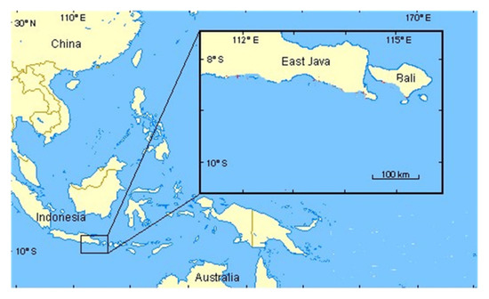
Figure 1.
Location of the East Java 150 kV power system.
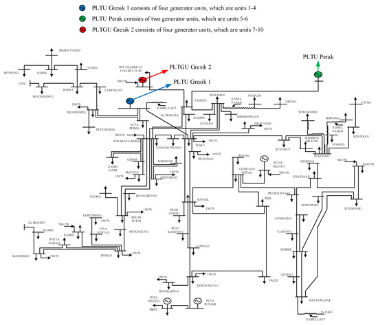
Figure 2.
Single line diagram of the East Java 150 kV power system.
The input data used in the fifth case study are shown in Table 13. Moreover, MIW-PSO is applied with total demand 616 MW. In this case study, the MIW-PSO is used to solve ED problems with smooth cost function. Using PSO obtain total cost 95,840.57. However, MIW-PSO gets 95,835.53 for total cost, as written in Table 14.
Table 13.
Generator unit capacity and coefficients on fifth case study.
Table 14.
Simulation result comparison on the fifth case study.
To validate accuracy of the MIW-PSO getting the optimal total cost, we computed the MIW-PSO in 100 trials. Figure 3 shows the accuracy validation of the MIW-PSO. Figure 3a represent the accuracy of the MIW-PSO in the first case study. MIW-PSO yields smaller generation cost deviation to obtain the optimal total cost, which is 8194.35513 $⁄hr. A similar thing is shown in Figure 3b–e, which represent the second to fifth case studies. Overall, through 100 trials for all case studies, it is shown that the MIW-PSO yields smaller generation costs deviation; thus, verifying that the MIW-PSO solution accuracy is acceptable stable.
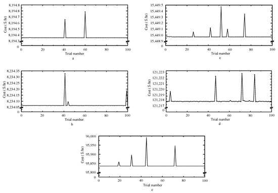
Figure 3.
The accuracy of the MIW-PSO: (a) first case study; (b) second case study; (c) third case study; (d) fourth case study; (e) fifth case study.
Convergence test is performed to verify the quickness of the proposed approach in terms of iterations number. Figure 4 depicts the convergence test of MIW-PSO. Figure 4a–e shows that the MIW-PSO has a good convergence ability; thus, obtaining good evaluation value of iteration and low generation cost. The MIW-PSO is consistently faster to convergence than the other algorithms, such as NM [51] for the first case study, MPSO [40] for the second case study, GA, PSO [24], NPSO, PSO-LRS, and NPSO-LRS [41] for the third case study, NPSO-LRS, IFEP, and FCEP [23] for the fourth case study, and the PSO for the fifth case study. Table 15 summarizes the comparison of the convergence test in terms of the number of iterations among different methods.
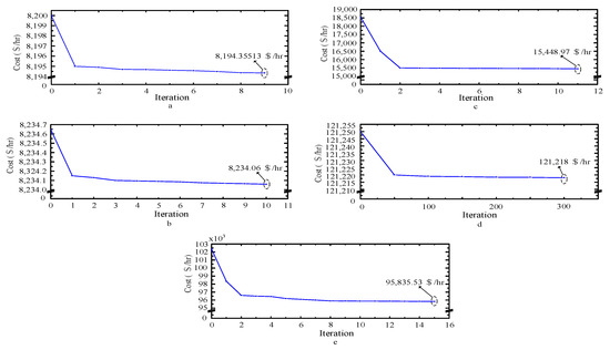
Figure 4.
The convergence of the MIW-PSO: (a) first case study; (b) second case study; (c) third case study; (d) fourth case study; (e) fifth case study.
Table 15.
Comparison of the convergence test among different methods.
In terms of computational efficiency, the comparison of the time computation is given in Table 16. Since some of the computation time of the other methods are not available, the comparison is just done with MHNN in the first case study, GA in the second case study, GA, PSO, and DE in the third case study, COPSO, NPSO, PSO-LRS, and NPSO LRS in the fourth case study, and PSO in the fifth case study. Besides the encoding, the computation time comparison is greatly influenced by the specifications of the computer in use. As shown in Table 15, the MIW-PSO has better computation time.
Table 16.
Comparison of computation time.
5. Discussion
In this study, six advantages are summarized as follow:
- An alternative method to solve the ED problem: this study applied a modified inertia weight on the PSO (MIW-PSO) algorithm. The MIW-PSO is proposed to solve the ED problems on generator scheduling;
- Perform well and considers the power generator characteristics: in order to solve the ED problems, the MIW-PSO performs well, and considers the power generator characteristics, such as smooth and non-smooth cost functions with prohibited operating zones and valve-point effects;
- Obtaining an optimal solution: in this study, the MIW-PSO shows excellent performance in order to obtain optimal solution, and at the same time, satisfy the constraints. In the first case study, the MIW-PSO obtains the total cost 8194.35513 . In the second case study, the MIW-PSO obtains the total cost 8234.06 . In third and fourth case studies, the MIW-PSO obtains the total cost 15,448.97 and 121,218 respectively. Finally, in the fifth case study, the MIW-PSO obtains total cost 95,835.53 ;
- Performing well and considers the power generator characteristics: the MIW-PSO performs well, and considers the power generator characteristics, such as smooth and non-smooth cost functions with prohibited operating zones and valve-point effects, in solving the ED problems;
- Extraordinary among other method approaches to solve ED problems: the obtained results of MIW-PSO are compared with the other methods, such as NM, MHNN, IEP, MPSO, GA, EP, PSO, PSO-LRS, NPSO-LRS, DE, IBSA, COPSO, DPD, IFEP, FCEP, IDE, MSOS, and NPSO. The MIW-PSO has better performance to obtain optimal results;
- Stable solution accuracy: through 100 trials, the MIW-PSO yields smaller generation cost deviation; thus, verifying that the MIW-PSO solution accuracy is acceptable stable.
- Faster to convergent: through the results of the convergence test, the MIW-PSO demonstrates the quickness of performance in terms of the number of iterations.
6. Conclusions
This study successfully shows the performance of a new MIW-PSO with incorporated chaotic search to solve the problems of ED. In the MIW-PSO, the approach of the constriction factor and inertia weight, along with the adjustment in the cognitive and social learning factors, are used together where a modification of inertia weight is introduced with an incorporation of the chaotic search strategy. Therefore, MIW-PSO makes ED problems effectively solved, satisfying the constraints, and makes optimal solutions greatly improved. The MIW-PSO is addressed to obtain an optimal total cost in solving the ED problems in optimal generator scheduling, while considering the smooth and non-smooth cost functions. Moreover, the method can also handle ED problems, considering POZ and VPE. The MIW-PSO has been demonstrated through five different case studies, is proven to have significant features, such as an optimal solution with stable solution accuracy, and offers the quickness of performance in terms of the number of iterations. The results of the five case studies show the superiority of the MIW-PSO compared with the results of several methods that have been published in the previous paper.
Author Contributions
Conceptualization, C.-Y.L. and M.T.; Methodology, C.-Y.L. and M.T.; Software, C.-Y.L. and M.T.; Validation, C.-Y.L. and M.T.; Formal Analysis, C.-Y.L. and M.T.; Investigation, C.-Y.L. and M.T.; Resources, C.-Y.L. and M.T.; Data Curation, C.-Y.L. and M.T.; Writing-Original Draft Preparation, C.-Y.L. and M.T.; Writing-Review & Editing, C.-Y.L. and M.T.; Visualization, C.-Y.L. and M.T.; Supervision, C.-Y.L.; Project Administration, C.-Y.L.; Funding Acquisition, C.-Y.L. All authors have read and agreed to the published version of the manuscript.
Funding
This research received no external funding.
Conflicts of Interest
The authors declare no conflict of interest.
References
- Chowdhury, B.H.; Rahman, S. A review of recent advances in economic dispatch. IEEE Trans. Power Syst. 1990, 5, 1248–1259. [Google Scholar] [CrossRef]
- Granville, S. Optimal reactive dispatch through interior point methods. IEEE Trans. Power Syst. 1994, 9, 136–146. [Google Scholar] [CrossRef]
- Tsekouras, G.J.; Kanellos, F.D.; Mastorakis, V.; Mladenow, V. Optimal operation of thermal electric power production system without transmission losses using Artificial Neural Networks based on augmented Lagrange multiplier method. In ICAN-2013, Lecture Notes in Computer Science 8131; Springer: Berlin/Heidelberg, Germany, 2013; pp. 586–594. [Google Scholar]
- Wang, M.Q.; Gooi, H.B.; Chen, S.X.; Lu, S. A mixed integer quadratic programming for dynamic economic dispatch with valve point effect. IEEE Trans. Power Syst. 2014, 29, 2097–2106. [Google Scholar] [CrossRef]
- Zhan, J.; Wu, Q.H.; Guo, C.; Zhou, X. Economic dispatch with non-smooth objectives—Part I: Local minimum analysis. IEEE Trans. Power Syst. 2015, 30, 710–721. [Google Scholar] [CrossRef]
- Zhan, J.; Wu, Q.H.; Guo, C.; Zhou, X. Economic dispatch with non-smooth objectives—Part II: Dimensional steepest decline method. IEEE Trans. Power Syst. 2015, 30, 722–733. [Google Scholar] [CrossRef]
- Yang, Y.; Wei, B.; Liu, H.; Zhang, Y.; Zhao, J.; Manla, E. Chaos firefly algorithm with self-adaptation mutation mechanism for solving large-scale economic dispatch with valve-point effects and multiple fuel options. IEEE Access 2018, 5, 45907–45922. [Google Scholar] [CrossRef]
- Liang, H.; Liu, Y.; Shen, Y.; Li, F.; Man, Y. A hybrid bat algorithm for economic dispatch with random wind power. IEEE Trans. Power Syst. 2018, 33, 5052–5061. [Google Scholar] [CrossRef]
- Shen, X.; Wu, G.; Wang, R.; Chen, H.; Li, H.; Shi, J. A self-adapted across neighborhood search algorithm with variable reduction strategy for solving non-convex static and dynamic economic dispatch problems. IEEE Access 2018, 6, 41314–41324. [Google Scholar] [CrossRef]
- Al-Betar, M.A.; Awadallah, M.A.; Khader, A.T.; Bolaji, A.L.A. Tournament-based harmony search algorithm for non-convex economic load dispatch problem. Appl. Soft Comput. 2016, 47, 449–459. [Google Scholar] [CrossRef]
- Al-Betar, M.A.; Awadallah, M.A.; Khader, A.T.; Bolaji, A.L.; Almomani, A. Economic load dispatch problems with valve-point loading using natural updated harmony search. Neural Comput. Appl. 2016, 29, 767–781. [Google Scholar] [CrossRef]
- Yan, S.L.; Gu, B.; Tian, D.X.; Ai, S.J. Hybrid biogeography constrained optimization for economic dispatch. Electr. Power Sci. Eng. 2016, 32, 31–36. [Google Scholar]
- Barisal, A.K.; Prusty, R.C. Large scale economic dispatch of power systems using oppositional invasive weed optimization. Appl. Soft Comput. 2015, 29, 122–137. [Google Scholar] [CrossRef]
- Lynn, N.; Suganthan, P.N. Heterogeneous comprehensive learning particle swarm optimization with enhanced exploration and exploitation. Swarm Evol. Comput. 2015, 24, 11–24. [Google Scholar] [CrossRef]
- Elsayed, W.T.; Hegazy, Y.G.; El-bages, M.S.; Bendary, F.M. Improved random drift particle swarm optimization with self-adaptive mechanism for solving the power economic dispatch problem. IEEE Trans. Ind. Inform. 2017, 13, 1017–1026. [Google Scholar] [CrossRef]
- Walters, D.C.; Sheble, G.B. Genetic algorithm solution of economic dispatch with valve point loading. IEEE Trans. Power Syst. 1993, 8, 1325–1332. [Google Scholar] [CrossRef]
- Chen, P.H.; Chang, H.C. Large-scale economic dispatch by genetic algorithm. IEEE Trans. Power Syst. 1995, 10, 1919–1926. [Google Scholar] [CrossRef]
- Chiang, C.L. Improved genetic algorithm for power economic dispatch of units with valve-point effects and multiple fuels. IEEE Trans. Power Syst. 2005, 20, 1690–1699. [Google Scholar] [CrossRef]
- Park, Y.M.; Won, J.R.; Park, J.B. A new approach to economic load dispatch based on improved evolutionary programming. Eng. Intell. Syst. Elect. Eng. Commun. 1998, 6, 103–110. [Google Scholar]
- Sinha, N.; Chakrabarti, R.; Chattopadhyay, P.K. Evolutionary programming techniques for economic load dispatch. IEEE Trans. Evol. Comput. 2003, 7, 83–94. [Google Scholar] [CrossRef]
- Wang, S.K.; Chiou, J.P.; Liu, C.W. Non-smooth/non-convex economic dispatch by a novel hybrid differential evolution algorithm. IET Gener. Transm. Distrib. 2017, 1, 793–803. [Google Scholar] [CrossRef]
- Elsayed, W.T.; El-Saadany, E.F. A Fully decentralized approach for solving the economic dispatch problem. IEEE Trans. Power Syst. 2015, 30, 2179–2189. [Google Scholar] [CrossRef]
- Basu, M. Fast convergence evolutionary programming for economic dispatch problems. IET Gener. Transm. Distrib. 2017, 11, 4009–4017. [Google Scholar] [CrossRef]
- Gaing, Z.L. Particle swarm optimization to solving the economic dispatch considering the generator constraints. IEEE Trans. Power Syst. 2003, 18, 1187–1195. [Google Scholar] [CrossRef]
- Zhao, J.; Wen, F.; Dong, Z.Y.; Xue, Y.; Wong, K.P. Optimal dispatch of electric vehicles and wind power using enhanced particle swarm optimization. IEEE Trans. Indus. Inf. 2012, 8, 889–899. [Google Scholar] [CrossRef]
- Niknam, T.; Golestaneh, F. Enhanced adaptive particle swarm optimization algorithm for dynamic economic dispatch of units considering valve-point effects and ramp rates. IET Gener. Transm. Distrib. 2012, 6, 424–435. [Google Scholar] [CrossRef]
- Chakraborty, S.; Senjyu, T.; Yona, A.; Saber, A.Y.; Funabashi, T. Solving economic load dispatch problem with valve-point effects using a hybrid quantum mechanics inspired particle swarm optimization. IET Gener. Transm. Distrib. 2011, 5, 1042–1052. [Google Scholar] [CrossRef]
- Li, C.; Yang, S.; Nguyen, T.T. A self-learning Particle swarm optimizer for global optimization problems. IEEE Trans. Syst. Man Cybern. Part B Cybern. 2012, 42, 627–646. [Google Scholar]
- Cong, T.D.; Zhijian, W. Adaptive multi-layer particle swarm optimization with neighborhood search. IET Chin. J. Electron. 2016, 25, 1079–1088. [Google Scholar]
- Hou, P.; Hu, W.; Soltani, M.; Chen, Z. Optimized placement of wind turbines in large-scale offshore wind farm using particle swarm optimization algorithm. IEEE Trans. Sustain. Energy 2015, 6, 1272–1282. [Google Scholar] [CrossRef]
- Crespo, J.M.; Usaola, J.; Fernandez, J.L. Security-constrained optimal generation scheduling in large-scale power systems. IEEE Trans. Power Syst. 2006, 21, 321–332. [Google Scholar] [CrossRef]
- Zhang, J.; Wang, J.; Yue, C. Small population-based particle swarm optimization for short-term hydrothermal scheduling. IEEE Trans. Power Syst. 2012, 27, 142–152. [Google Scholar] [CrossRef]
- Hu, M.; Wu, T.; Weir, J.D. An adaptive particle swarm optimization with multiple adaptive methods. IEEE Trans. Evol. Comput. 2013, 17, 705–720. [Google Scholar] [CrossRef]
- Abbas, G.; Gu, J.; Farooq, U.; Asad, M.U.; El-Harawy, M. Solution of an economic dispatch problem through particle swarm optimization: A detailed survey-part I. IEEE Access 2017, 5, 15105–15141. [Google Scholar] [CrossRef]
- Abbas, G.; Gu, J.; Farooq, U.; Raza, A.; Asad, M.U.; El-Harawy, M. Solution of an economic dispatch problem through particle swarm optimization: A detailed survey-part II. IEEE Access 2017, 5, 24426–24445. [Google Scholar] [CrossRef]
- Vlachogiannis, J.G.; Lee, K.Y. A comparative study on particle swarm optimization for optimal steady-state performance of power system. IEEE Trans. Power Syst. 2006, 21, 1718–1728. [Google Scholar] [CrossRef]
- Yumbla, P.E.O.; Ramirez, J.M.; Coello, C.A. Optimal power flow Subject to security constraints solved with a particle swarm optimizer. IEEE Trans. Power Syst. 2008, 23, 33–40. [Google Scholar] [CrossRef]
- Sun, J.; Palade, V.; Xiao, J.W.; Fang, W.; Wang, Z. Solving the power economic dispatch problem with generator constraints by random drift particle swarm optimization. IEEE Trans. Ind. Inf. 2014, 10, 222–232. [Google Scholar] [CrossRef]
- Kuo, C.C. A novel coding scheme for practical economic dispatch by modified particle swarm approach. IEEE Trans. Power Syst. 2008, 23, 1825–1835. [Google Scholar]
- Park, J.B.; Lee, K.S.; Shin, J.R.; Lee, K.Y. A particle swarm optimization for economic dispatch with nonsmooth cost functions. IEEE Trans. Power Syst. 2005, 20, 34–42. [Google Scholar] [CrossRef]
- Selvakumar, A.I.; Thanushkodi, K. A new particle swarm optimization solution to nonconvex economic dispatch problems. IEEE Trans. Power Syst. 2007, 22, 45–51. [Google Scholar] [CrossRef]
- Yang, H.T.; Yang, P.C.; Huang, C.L. Evolutionary programming based economic dispatch for units with non-smooth fuel cost functions. IEEE Trans. Power Syst. 1996, 11, 112–118. [Google Scholar] [CrossRef]
- Shi, Y.; Eberhart, R.C. Empirical study of particle swarm optimization. In Proceedings of the Congress on Evolutionary Computation -CEC99 (Cat. No. 99TH8406), Washington, DC, USA, 6–9 July 1999. [Google Scholar]
- Naka, S.; Genji, T.; Yura, T.; Fukuyama, Y. A hybrid particle swarm optimization for distribution state estimation. IEEE Trans. Power Syst. 2003, 22, 60–68. [Google Scholar] [CrossRef]
- He, S.; Wu, Q.H.; Wen, J.Y.; Saunders, J.R.; Patton, P.C. A particle swarm optimizer with passive congregation. Biosystems 2004, 78, 135–147. [Google Scholar] [CrossRef] [PubMed]
- Shi, Y.; Eberhart, R.C. Comparing inertia weights and constriction factors in particle swarm optimization. In Proceedings of the IEEE Congress on Evolutionary Computation (CEC2000), La Jolla, CA, USA, 16–19 July 2000; pp. 84–88. [Google Scholar]
- Zhan, Z.H.; Zhang, J.; Li, Y.; Chung, H.S.H. Adaptive particle swarm optimization. IEEE Trans. Syst. Man Cybern. Part B 2009, 39, 1362–1381. [Google Scholar] [CrossRef]
- Taherkhani, M.; Safabakhsh, R. A novel stability-based adaptive inertia weight for particle swarm optimization. Appl. Soft Comput. 2016, 38, 281–295. [Google Scholar] [CrossRef]
- Caponetto, R.; Fortuna, L.; Fazzino, S.; Xibilia, M.G. Chaotic sequences to improve the performance of evolutionary algorithms. IEEE Trans. Evol. Comput. 2003, 7, 289–304. [Google Scholar] [CrossRef]
- Park, J.B.; Lee, K.S.; Shin, J.R.; Lee, K.Y. An improved particle swarm optimisation for nonconvex economic dispatch problems. IEEE Trans. Power Syst. 2010, 25, 156–166. [Google Scholar] [CrossRef]
- Lee, C.Y.; Tuegeh, M. Optimal optimisation-based microgrid scheduling considering impacts of unexpected forecast errors due to the uncertainty of renewable generation and loads fluctuation. IET Renew. Power Gener. 2020, 14, 321–331. [Google Scholar] [CrossRef]
- Wood, A.J.; Wollenberg, B.F. Power Generation, Operational and Control, 2nd ed.; Jhon Wiley & Sons Inc.: Hoboken, NJ, USA, 1996. [Google Scholar]
- Fu, C.; Zhang, S.; Chao, K.H. Energy management of a power system for economic load dispatch using the artificial intelligent algorithm. Electronics 2020, 9, 108. [Google Scholar] [CrossRef]
- Parouha, R.P.; Das, K.N. DPD: An intelligent parallel hybrid algorithm for economic load dispatch problems with various practical constraints. Expert Syst. Appl. 2016, 63, 295–309. [Google Scholar] [CrossRef]
- Zou, D.; Li, S.; Wang, G.G.; Li, Z.; Ouyang, H. An improved differential evolution algorithm for the economic load dispatch problems with or without valve-point effects. Appl. Energy 2016, 181, 375–390. [Google Scholar] [CrossRef]
- Secui, D.C. A modified symbiotic organisms search algorithm for large scale economic dispatch problem with valve-point effects. Energy 2016, 113, 366–384. [Google Scholar] [CrossRef]
- Chen, X.; Xu, B.; Du, W. An Improved particle swarm optimization with biogeography-based learning strategy for economic dispatch problems. Complexity 2018, 2018, 7289674. [Google Scholar] [CrossRef]
© 2020 by the authors. Licensee MDPI, Basel, Switzerland. This article is an open access article distributed under the terms and conditions of the Creative Commons Attribution (CC BY) license (http://creativecommons.org/licenses/by/4.0/).