Forecasting Hierarchical Time Series in Power Generation

Abstract

Academic attention is being paid to the study of hierarchical time series. Especially in the electrical sector, there are several applications in which information can be organized into a hierarchical structure. The present study analyzed hourly power generation in Brazil (2018–2020), grouped according to each of the electrical subsystems and their respective sources of generating energy. The objective was to calculate the accuracy of the main measures of aggregating and disaggregating the forecasts of the Autoregressive Integrated Moving Average (ARIMA) and Error, Trend, Seasonal (ETS) models. Specifically, the following hierarchical approaches were analyzed: (i) bottom-up (BU), (ii) top-down (TD), and (iii) optimal reconciliation. The optimal reconciliation models showed the best mean performance, considering the primary predictive windows. It was also found that energy forecasts in the South subsystem presented greater inaccuracy compared to the others, which signals the need for individualized models for this subsystem.

1. Introduction

The advent of Industry 4.0 revolutionized factories worldwide, since it allowed the connectivity between measuring machines and the automation of companies, distributing the capacity to collect massive volumes of data [1]. In high-level data analysis, forecasting models allow the extraction of behavior patterns, as well as the prediction of future values for the collected data set [2].

In the above-mentioned scenario, the construction of predictive models is gaining prominence in the literature [3,4,5], since economic agents deal with uncertainty in multiple spheres and aim to achieve the best results using available resources [6]. Developing acceptably accurate models presents a meaningful challenge, as prediction is a technique that deals with risk and there will always be a fundamental error associated with it. The best model is the one that most adequately represents the phenomenon of interest.

In relation to the object of our study, power generation, there are several forecasting applications: (i) classical time series models like the autoregressive moving average, autoregressive integrated moving average, and generalized autoregressive conditional heteroscedastic among others [7,8]; (ii) pre-processing techniques like spectrum analysis, wavelets, and Fourier analysis [9]; and, (iii) machine learning approaches such as neural networks, fuzzy systems, and support vector machine [10]. Alternatively, hybrid models aim to combine machine learning representations with different methods. These methods include focused time-delay neural networks [11], wavelet neuro-fuzzy systems [12], finite-impulse response neural networks [13], local feedback dynamic fuzzy neural networks [14], type recurrent fuzzy networks [15], and neuro-fuzzy inference systems [16] among others.

Additionally, an alternative class known as hierarchical forecasting [17,18,19] deals with organized time series that can be aggregated at different levels into groups based on geography, sources of energy, or other, specific features. Despite this being a recent topic, there is already research that has addressed the use of hierarchical forecasting models in the energy sector. Examples of hierarchical forecasting include electrical grids [20], solar power generation [21], energy transport [22], short-term load forecasting [23], long-term load forecasting [24], energy consumption [25], and air pollution [26] among others.

The papers identified above have calibrated the forecasts using only the bottom-up, top-down or Ordinary least squares (OLS) assumptions [19]. Thus, the following research question is formulated: how is it possible to make hierarchical predictions using advanced linear regression models with regularization? In this way, it is expected to obtain more reliable forecasts by rewriting the hierarchical problem in terms of finding a set of unbiased, minimum variance measures of projected values across the whole array of data. It is possible to minimize the sum of variances of the reconciled estimate errors under the property of unbiasedness, using the procedure called MinT (minimum trace) reconciliation [27].

The present paper presents a case study using a power generation data set from Brazil (2018–2020) organized by electrical subsystems and different generating sources. Specifically, the main approaches used to aggregate and disaggregate predictions made for grouped time series are examined, namely: (i) bottom-up, (ii) top-down and (iii) optimal reconciliation models (OLS, WLS and MinT). The ARIMA and ETS predictive models were used to test the performance of these reconciliation methods, since these are the default models available in the R-package HTS. Further descriptions can be found in the materials and methods section.

The remainder of the present paper is organized as follows. Section 2 defines the study methodology, describing the data set, hierarchical procedures, and forecasting models employed. Section 3 presents the results and discussions of the techniques, in addition to the limitations of this paper. Finally, Section 4 presents the conclusions and guidelines for future work.

2. Materials and Methods

The secondary data used in this study correspond to the amounts of power generated by each of the Brazilian electrical subsystems (North, Northeast, Southeast/Midwest, and South). We separated these data according to the source of energy (wind, hydroelectric, thermal, solar, and nuclear). Data were obtained from the National Electric System Operator [28], due to their reliability. The observations of hourly power generation (GWh) were made during the period from January 2018 to January 2020, making a total of 17,521 h.

Based on Hyndman et al. [19], we present a schematic representation of the Brazilian energy generation system, comprising a three-level hierarchical structure (Figure 1). Level 0 represents the total energy generated in Brazil (completely aggregated series). Level 1 denotes each of Brazil’s electrical subsystems (first level of disaggregation). The last level, Level 2, represents each of the energy generating sources (Level k). According to this framework, it is possible to identify the most disaggregated time series (in this case k = 2).

Table 1. Amounts of power generation in Brazil (GWh).

Subsystem/Source		Wind	Hydro	Thermal	Solar	Nuclear	Total (GWh—Subsystem)	%
North	(A)	2688	125,182	31,489	0	0	159,359	14.3%
Northeast	(B)	85,377	37,705	36,699	4626	0	164,407	14.7%
Southeast/Midwest	(C)	0	518,714	73,555	2437	31,805	626,511	56.1%
South	(D)	11,326	135,914	19,472	0	0	166,712	14.9%
Total (GWh—Source)		99,391	817,516	161,215	7063	31,805	1,116,989	100%
%		8.9%	73.2%	14.4%	0.6%	2.8%	100%	-

shows the amounts of power generation in Brazil (GWh), according to generating sources and electrical subsystems. There is a predominance of hydroelectric generation (73%), making the Brazilian electrical matrix one of the cleanest in the world. At the same time, the Southeast/Midwest subsystem accounts for more than half (56%) of all energy generated in the country.

Routines were implemented using the R^® programming language [29]. The R-package HTS was used to calculate the bottom-up, top-down, optimal combination reconciliation and trace minimization reconciliation. HTS is available at: https://cran.r-project.org/web/packages/hts/index.html. Although HTS includes functions for creating, plotting and forecasting hierarchical time series, it has some limitations. Those limitations include the fact that it has only three built-in forecasting options: ARIMA, ETS, and random walks [19]. This paper will use the ARIMA and the ETS models since they have automatic adjustment and allow consideration of factors such as the trend and seasonality of the data set. The computer used to execute the algorithms had CPU Intel Core i5-7200 2.70 GHz, RAM of 16 GB, and operating system Windows 10 x64. In the next subsection, we present the hierarchical reconciliation models used in the present paper, as well as the forecasting models.

2.1. The Bottom-Up (BU) Approach

The BU procedure requires first providing forecasts for every series at the bottom-level, and then summing these to generate forecasts for all the levels of the hierarchical structure [30]. In its simplicity, this approach neglects the relations between time series and works, mainly unsuccessfully, on highly disaggregated data. These data tend to have a low signal-to-noise ratio [27]. According to the hierarchy (Figure 1), we first make h-step-ahead forecasts for all the bottom-level time series (n = 14):

$${\widehat{y}}_{AA,t},{\widehat{y}}_{AB,t},{\widehat{y}}_{AC,t},{\widehat{y}}_{BA,t},{\widehat{y}}_{BB,t},{\widehat{y}}_{BC,t},{\widehat{y}}_{BD,t},{\widehat{y}}_{CA,t},{\widehat{y}}_{CB,t},{\widehat{y}}_{CC,t},{\widehat{y}}_{CD,t},{\widehat{y}}_{DA,t},{\widehat{y}}_{DB,t},{\widehat{y}}_{DC,t}.$$

(1)

Summing these, we obtain h-step-ahead forecasts for the rest of the series:

$$\begin{gathered} {\tilde{y}}_t={\widehat{y}}_{AA,t}+{\widehat{y}}_{AB,t}+{\widehat{y}}_{AC,t}+{\widehat{y}}_{BA,t}+{\widehat{y}}_{BB,t}+{\widehat{y}}_{BC,t}+{\widehat{y}}_{BD,t}+{\widehat{y}}_{CA,t}+{\widehat{y}}_{CB,t} \\ +{\widehat{y}}_{CC,t}+{\widehat{y}}_{CD,t}+{\widehat{y}}_{DA,t}+{\widehat{y}}_{DB,t}+{\widehat{y}}_{DC,t}. \\ {\tilde{y}}_{A,t}={\widehat{y}}_{AA,t}+{\widehat{y}}_{AB,t}+{\widehat{y}}_{AC,t}. \\ {\tilde{y}}_{B,t}={\widehat{y}}_{BA,t}+{\widehat{y}}_{BB,t}+{\widehat{y}}_{BC,t}+{\widehat{y}}_{BD,t}. \\ {\tilde{y}}_{C,t}={\widehat{y}}_{CA,t}+{\widehat{y}}_{CB,t}+{\widehat{y}}_{CC,t}+{\widehat{y}}_{CD,t}. \\ {\tilde{y}}_{D,t}={\widehat{y}}_{DA,t}+{\widehat{y}}_{DB,t}+{\widehat{y}}_{DC,t}. \end{gathered}$$

(2)

According to [19], it is possible to arrange the equations expressed in (2) into an algebra notation. Below is a complete notation for this problem:

$$\left[\begin{array}{c}{\tilde{y}}_t\\ {\tilde{y}}_{A,t}\\ {\tilde{y}}_{B,t}\\ {\tilde{y}}_{C,t}\\ {\tilde{y}}_{D,t}\\ {\tilde{y}}_{AA,t}\\ {\tilde{y}}_{AB,t}\\ {\tilde{y}}_{AC,t}\\ {\tilde{y}}_{BA,t}\\ {\tilde{y}}_{BB,t}\\ {\tilde{y}}_{BC,t}\\ {\tilde{y}}_{BD,t}\\ {\tilde{y}}_{CA,t}\\ {\tilde{y}}_{CB,t}\\ {\tilde{y}}_{CC,t}\\ {\tilde{y}}_{CD,t}\\ {\tilde{y}}_{DA,t}\\ {\tilde{y}}_{DB,t}\\ {\tilde{y}}_{DC,t}\end{array}\right]=\left[\begin{array}{cccccccccccccc}1& 1& 1& 1& 1& 1& 1& 1& 1& 1& 1& 1& 1& 1\\ 1& 1& 1& 0& 0& 0& 0& 0& 0& 0& 0& 0& 0& 0\\ 0& 0& 0& 1& 1& 1& 1& 0& 0& 0& 0& 0& 0& 0\\ 0& 0& 0& 0& 0& 0& 0& 1& 1& 1& 1& 0& 0& 0\\ 0& 0& 0& 0& 0& 0& 0& 0& 0& 0& 0& 1& 1& 1\\ 1& 0& 0& 0& 0& 0& 0& 0& 0& 0& 0& 0& 0& 0\\ 0& 1& 0& 0& 0& 0& 0& 0& 0& 0& 0& 0& 0& 0\\ 0& 0& 1& 0& 0& 0& 0& 0& 0& 0& 0& 0& 0& 0\\ 0& 0& 0& 1& 0& 0& 0& 0& 0& 0& 0& 0& 0& 0\\ 0& 0& 0& 0& 1& 0& 0& 0& 0& 0& 0& 0& 0& 0\\ 0& 0& 0& 0& 0& 1& 0& 0& 0& 0& 0& 0& 0& 0\\ 0& 0& 0& 0& 0& 0& 1& 0& 0& 0& 0& 0& 0& 0\\ 0& 0& 0& 0& 0& 0& 0& 1& 0& 0& 0& 0& 0& 0\\ 0& 0& 0& 0& 0& 0& 0& 0& 1& 0& 0& 0& 0& 0\\ 0& 0& 0& 0& 0& 0& 0& 0& 0& 1& 0& 0& 0& 0\\ 0& 0& 0& 0& 0& 0& 0& 0& 0& 0& 1& 0& 0& 0\\ 0& 0& 0& 0& 0& 0& 0& 0& 0& 0& 0& 1& 0& 0\\ 0& 0& 0& 0& 0& 0& 0& 0& 0& 0& 0& 0& 1& 0\\ 0& 0& 0& 0& 0& 0& 0& 0& 0& 0& 0& 0& 0& 1\end{array}\right]\left[\begin{array}{c}{\widehat{y}}_{AA,t}\\ {\widehat{y}}_{AB,t}\\ {\widehat{y}}_{AC,t}\\ {\widehat{y}}_{BA,t}\\ {\widehat{y}}_{BB,t}\\ {\widehat{y}}_{BC,t}\\ {\widehat{y}}_{BD,t}\\ {\widehat{y}}_{CA,t}\\ {\widehat{y}}_{CB,t}\\ {\widehat{y}}_{CC,t}\\ {\widehat{y}}_{CD,t}\\ {\widehat{y}}_{DA,t}\\ {\widehat{y}}_{DB,t}\\ {\widehat{y}}_{DC,t}\end{array}\right]$$

(3)

Alternatively, the notation presented in (3) can be reformulated in a compact way by applying the summing matrix. Thus, the bottom-up approach can be represented as:

$${\tilde{y}}_t=S{\widehat{b}}_t,$$

(4)

where ${\tilde{y}}_t$ is an $n$-dimensional vector of $h$-step-ahead forecasts for the total energy, S is the summing matrix, and ${\widehat{b}}_t$ is an $m$-dimensional vector of $h$-step-ahead forecasts for each of the sources of energy at bottom-level. An advantage of this procedure is that we are forecasting at the bottom-level of a hierarchy. Consequently, no information is missed due to aggregation [17].

2.2. The Top-Down (TD) Approach

Top-down methods operate with strictly hierarchical aggregation structures, not with grouped structures. They involve first making forecasts for the Total level $y_t$, and next disaggregating these down the hierarchy [17]. Let $p_1,\dots ,p_m$ be a set of disaggregation proportions that deliver the forecasts of the Total series, which are to be distributed in order to obtain forecasts for all series at the bottom-level of the structure. To illustrate, concerning our hierarchy by applying proportions to Figure 1, we get $p_1,\dots ,p_{14}$:

$$\begin{gathered} {\tilde{y}}_{AA,t}=p_1{\widehat{y}}_t,{\tilde{y}}_{AB,t}=p_2{\widehat{y}}_t,{\tilde{y}}_{AC,t}=p_3{\widehat{y}}_t. \\ {\tilde{y}}_{BA,t}=p_4{\widehat{y}}_t,{\tilde{y}}_{BB,t}=p_5{\widehat{y}}_t,{\tilde{y}}_{BC,t}=p_6{\widehat{y}}_t,{\tilde{y}}_{BD,t}=p_7{\widehat{y}}_t. \\ {\tilde{y}}_{CA,t}=p_8{\widehat{y}}_t,{\tilde{y}}_{CB,t}=p_9{\widehat{y}}_t,{\tilde{y}}_{CC,t}=p_{10}{\widehat{y}}_t,{\tilde{y}}_{CD,t}=p_{11}{\widehat{y}}_t. \\ {\tilde{y}}_{DA,t}=p_{12}{\widehat{y}}_t,{\tilde{y}}_{DB,t}=p_{13}{\widehat{y}}_t,{\tilde{y}}_{DC,t}=p_{14}{\widehat{y}}_t. \end{gathered}$$

(5)

This can be rewritten using matrix notation. If we stack the set of proportions in an m-dimensional vector $p={(p_1,\dots ,p_m)}^{\prime }$, we have the bottom-level h-step-ahead predictions. Overall, for a given set of proportions, top-down approaches can be written as:

$$\begin{gathered} {\tilde{b}}_t=p_j{\widehat{y}}_t. \\ {\tilde{y}}_t=S{p}_j{\widehat{y}}_t. \end{gathered}$$

(6)

The main TD models stipulate disaggregation proportions according to the historical proportions of the data. Among the main models of this approach, we highlight the following three: (i) top-down Gross–Sohl method A (TDGSA), (ii) top-down Gross–Sohl method F (TDGSF), and (iii) Top-down forecast proportions (TDFP) (

Table 2. TD disaggregation proportions according to the historical proportions of the data.

TD Gross-Sohl Method A TDGSA	TD Gross-Sohl Method F TDGSF	TD Forecast Proportions TDFP
$p_j=\frac{1}{T}{\displaystyle \sum _{t=1}^T}\frac{y_{j,t}}{y_t}$	$p_j={\displaystyle \sum _{t=1}^T}\frac{y_{j,t}}{T}/{\displaystyle \sum _{t=1}^T}\frac{y_t}{T}$	$p_j={\displaystyle \prod _{l=0}^{K-1}}\frac{{\widehat{y}}_{j,t}^{(l)}}{{\widehat{S}}_{j,t}^{(l+1)}}$
for $j=1,\dots ,m$. Each proportion $p_j$ reflects the average of the historical proportions of the bottom-level series $y_{j,t}$ , t over the period $t=1,\dots ,T$ relative to the total aggregate $y_t$.	for $j=1,\dots ,m$. Each proportion $p_j$ takes the average historical value of the bottom-level series $y_{j,t}$ related to the average value of the total aggregate $y_t$.	where $j=1,\dots ,m$, ${\widehat{y}}_{j,h}^{(l)}$ is the $h$-step-ahead forecast and ${\widehat{S}}_{j,t}^{(l)}$ is the sum of the $h$-step-ahead forecasts below the node that is $l$ levels above node $j$.

). Additional details and demonstrations of Table 2 can be obtained from [18,31].

2.3. The Optimal Reconciliation Approaches

The optimal reconciliation approach proposed by [19] consists of an ordinary least squares problem based on the calculation of independent projections for all hierarchical levels, then applying a regression model to optimize the combination of these forecasts. According to [32], we can write the base prediction as:

$${\widehat{y}}_{t+h|t}=S{\beta }_{t+h|t}+{\epsilon }_h,$$

(7)

where ${\beta }_{t+h|t}$ represents the unknown conditional mean of the most disaggregated series, and ${\epsilon }_h$ is the error with mean of zero and covariance matrix ${\sum }_h$. If ${\sum }_h$ were known, the estimator of ${\beta }_{t+h|t}$ would lead to the following weighted least squares, producing reconciled forecasts, as follows:

$${\tilde{y}}_{t+h|t}=S{\widehat{\beta }}_{t+h|t}=S{(S^{\prime }{\sum }_h^{-1}S)}^{-1}{S}^{\prime }{\sum }_h^{-1}{\widehat{y}}_{t+h|t}=SP{\widehat{y}}_{t+h|t},$$

(8)

where $P={(S^{\prime }{\sum }_h^{-1}S)}^{-1}{S}^{\prime }{\sum }_h^{-1}S$. If the base forecasts ${\widehat{y}}_{t+h|t}$ are unbiased, then the reconciled forecasts ${\tilde{y}}_{t+h|t}$ will be unbiased, provided that $SPS=S$ [19]. This condition is valid for this reconciliation procedure for the bottom-up, although not for the top-down, methods. Consequently, the top-down approaches will never give unbiased reconciled forecasts, even if the base forecasts are unbiased. Additionally, [27] proved that, in general, $\sum h$ is not known and not identifiable. The covariance matrix of the $h$-step-ahead reconciled forecast errors is given by the following expression:

$$Va{r}_{(y_{t+h}-{\tilde{y}}_{t+h|t})}=SP{W}_h{P}^{\prime }{S}^{\prime },$$

(9)

for any $P$ such that $SPS=S$, then $W_h=Va{r}_{(y_{t+h}-{\widehat{y}}_{t+h|t})}=E({\widehat{e}}_{t+h|t}{{\widehat{e}}^{\prime }}_{t+h|t})$ is the covariance matrix of the corresponding h-step ahead base forecast errors. The purpose is to get the matrix P that minimizes the error variances of the reconciled forecasts which are on the diagonal of the covariance matrix $Va{r}_{(y_{t+h}-{\tilde{y}}_{t+h|t})}$. Finally, [27] demonstrated that the optimal reconciliation matrix P that minimizes the trace of $SP{W}_h{P}^{\prime }{S}^{\prime }=$, such that $SPS=S$, and the optimal reconciled forecasts, respectively, are given by:

$$\begin{gathered} P={(S^{\prime }{W_h}^{-1}S)}^{-1}{S}^{\prime }{W_h}^{-1} \\ {\tilde{y}}_{t+h|t}=S{(S^{\prime }{W_h}^{-1}S)}^{-1}{\mathrm{S}}^{\prime }{W_h}^{-1}{\widehat{y}}_{t+h|t}, \end{gathered}$$

(10)

which is introduced as the MinT (minimum trace) estimator. The next step consists of estimating $W_h$, a matrix of order $n$. Wickramasuriya, Athanasopoulos and Hyndman [27] proposed the following procedures (

Table 3. Hierarchical forecasting for electricity generation based on the ARIMA procedure.

Procedure	Description
OLS	$W_h=k_{h}I,\forall h$ where $k_h>0$. This is the most simplifying premise, and collapses the MinT estimator to the OLS estimator, proposed by Hyndman et al. [19]. This is optimal when the base forecast errors are uncorrelated and equivariant.
WLSv	$W_h=k_h\text{diag}({\widehat{W}}_1),\forall h$ where $k_h>0$ and: $\widehat{W}=\frac{1}{T}{\sum }_{t=1}^T{\widehat{e}}_t(1){\widehat{e}}_t{(1)}^{\prime }$, is the unbiased sample covariance estimator of the in-sample one-step-ahead base forecast errors. In this case, we can describe MinT as a WLS estimator applying variance scaling [27].
WLSs	$W_h=k_h\Lambda ,\forall h$ where $k_h>0$ and $\Lambda =\text{diag}(S1)$ with $1$ being a unit column vector of dimension $n$. We assume that each of the bottom-level base forecast errors has a variance $k_h$ and is uncorrelated between nodes. Consequently, every element of the diagonal $\Lambda$ matrix receives the number of forecast error variances contributing to that aggregation level [27]. This estimator depends only on the grouping structure of the hierarchy.
MinT (Sample)	$W_h=k_w{\widehat{W}}_1,\forall h$ where $k_h>0$, the unrestricted sample covariance estimator for $h=1$ [27]. In the results section, we denote this as MinT (Sample).
MinT (Shrink)	$W_h=k_w\widehat{W_{1,D}^{*}};\forall h$; $k_h>0;W_{1,D}^{*}={\lambda }_D{\widehat{W}}_{1,D}+(1-{\lambda }_D){\widehat{W}}_1$, is a shrinkage estimator with diagonal target, ${\widehat{W}}_{1,D}$, which is a diagonal matrix comprising the diagonal entries of ${\widehat{W}}_1$, and ${\lambda }_D$ is the shrinkage intensity parameter. Thus, off-diagonal elements of ${\widehat{W}}_1$ are shrunk toward zero and diagonal elements (variances) remain unchanged [27]. Wickramasuriya, Athanasopoulos and Hyndman [27] suggested a scale and location invariant shrinkage estimator by parameterizing the shrinkage in terms of variances and correlations: ${\widehat{\lambda }}_D=\frac{{\sum }_{i\ne j}{\widehat{var}}_{({\widehat{r}}_{ij})}}{{\sum }_{i\ne j}{{\widehat{r}}^2}_{ij}}$, where ${\widehat{r}}_{ij}$ is the $ij$th element of ${\widehat{R}}_1$, the $1$-step-ahead sample correlation matrix to shrink it toward an identity matrix.

Source: adapted by authors from: [27].

) to obtain the matrix:

2.4. ARIMA and ETS Formulation

ARIMA is one of the most-widely-used time series approaches for forecasting power generation [33]. Although studies have shown that ETS outperforms ARIMA [34], it is recommended to keep ARIMA as a reference model during the forecasting process. Moreover, several statistical software packages, like R^®, provide automatic model identification and parameter estimation skills for both ARIMA and ETS [17]. Professor Hyndman [19] developed the HTS package initially based on these predictive models. The present paper aims to test different approaches to optimal forecast reconciliation and, to do so, only the ARIMA and ETS models will be used. It is recommended that future studies extend these forecasting procedures using different predictive models, such as machine learning ones.

ARIMA was proposed by [33]. It is a linear forecasting method for dealing with stationary time series [34]. In the initial step, a time series is built stationary by differencing $d$ times along with some nonlinear transformations, such as logging [34]. The consequential data are recognized as a linear function of past $p$ data values and $q$ errors (11), i.e., modeled as an autoregressive moving average (ARMA) model,

$$y_t={\varnothing }_1{y}_{t-1}+{\varnothing }_2{y}_{t-2}+\dots +{\varnothing }_p{y}_{t-p}+{\Theta }_1{\epsilon }_{t-1}+{\Theta }_2{\epsilon }_{t-2}+\dots +{\Theta }_q{\epsilon }_{q-1},$$

(11)

where $y_t$ denotes real value at time $t$, ${\epsilon }_t$ describes the error sequence: it is supposed to be white noise and Gaussian distributed $(0,{\sigma }^2)$. ${\varnothing }_i$ for $(i=1,2,\dots ,p)$ are autoregressive $(AR)$ coefficients and ${\Theta }_j$ for $(j=1,2,\dots ,q)$ are moving average $(MA)$ coefficients. $p$ and $q$ are integers referred to as model orders. The time series model is denoted as $ARIMA(p,d,q)$ [35,36].

According to [34], the group of exponential smoothing methods utilizes the principle of weighted averages of past information for making forecasts. Since its formulation in 1950, a variety of exponential smoothing methods have been developed. All exponential smoothing methods were initially classified by [37], which has been continued by [38,39,40]. ETS stands for error, trend, and seasonality elements. As pointed by [34], the usual representation for these patterns involves a state vector $x_t={(l_t,b_t,s_t,s_{t-1},\dots ,s_{t-m+1})}^{\prime }$, and the state space equations [39] have the resulting structure:

$$\begin{gathered} y_t=w(x_{t-1})+r(x_{t-1}){\epsilon }_t \\ {x}_t=f(x_{t-1})+g(x_{t-1}){\epsilon }_t, \end{gathered}$$

(12)

where $({\epsilon }_t)$ denotes a Gaussian white noise $(0,{\sigma }^2)$ and ${\mu }_t=w(x_t-1)$. The model with additive error has $r_t(x_t-1)=1$, so $y_t={\mu }_t+{\epsilon }_t$. The model with multiplicative errors has $r_t(x_t-1)={\mu }_t$ = 𝜇𝑡, so $y_t={\mu }_t(1+{\epsilon }_t)$. Consequently, ${\epsilon }_t=(y_t-{\mu }_t)∕{\mu }_t$ is a relative error for the multiplicative model and any value of $r_t(x_t-1)$ will lead to the identical point forecast for $y_t$ [34,39].

2.5. Evaluating Forecast Accuracy

According to [20], there are several accuracy metrics, such as mean absolute percentage error (MAPE), mean absolute error (MAE), mean absolute scaled error (MASE), or root-mean-square error (RMSE), to evaluate the performance of point prediction methods, defined as follows:

$$MAPE=\frac{1}{T}{\sum }_{t=1}^T\left|\frac{y_t-{\widehat{y}}_t}{y_t}\right|.$$

(13)

$$MAE=\frac{1}{T}{\sum }_{t=1}^T\left|y_t-{\widehat{y}}_t\right|.$$

(14)

$$MASE=\frac{MAE}{MA{E}_{in-sample,naive}}$$

(15)

$$RMSE=\sqrt{\frac{1}{T}{\sum }_{t=1}^T{(y_t-{\widehat{y}}_t)}^2},$$

(16)

where $y_t$ is the amount of power generation at time t, ${\widehat{y}}_t$ is the fitted value for power generation, and $MA{E}_{in-sample,naive}$ is the MAE generated by a naive forecast.

Specifically, in studies of hierarchical time series, the MAPE indicator appears the most frequently in the literature [41,42,43]. MAPE was also the selected metric for the present paper (Figure 2 and Figure 3). Complementarily, MAE, MASE, and RMSE were estimated, and the results can be found in the Appendix A (Figure A3 and Figure A4). The values of the MAPE, MAE, MASE and RMSE statistics were obtained using a weighted average, with proportions from Table 1.

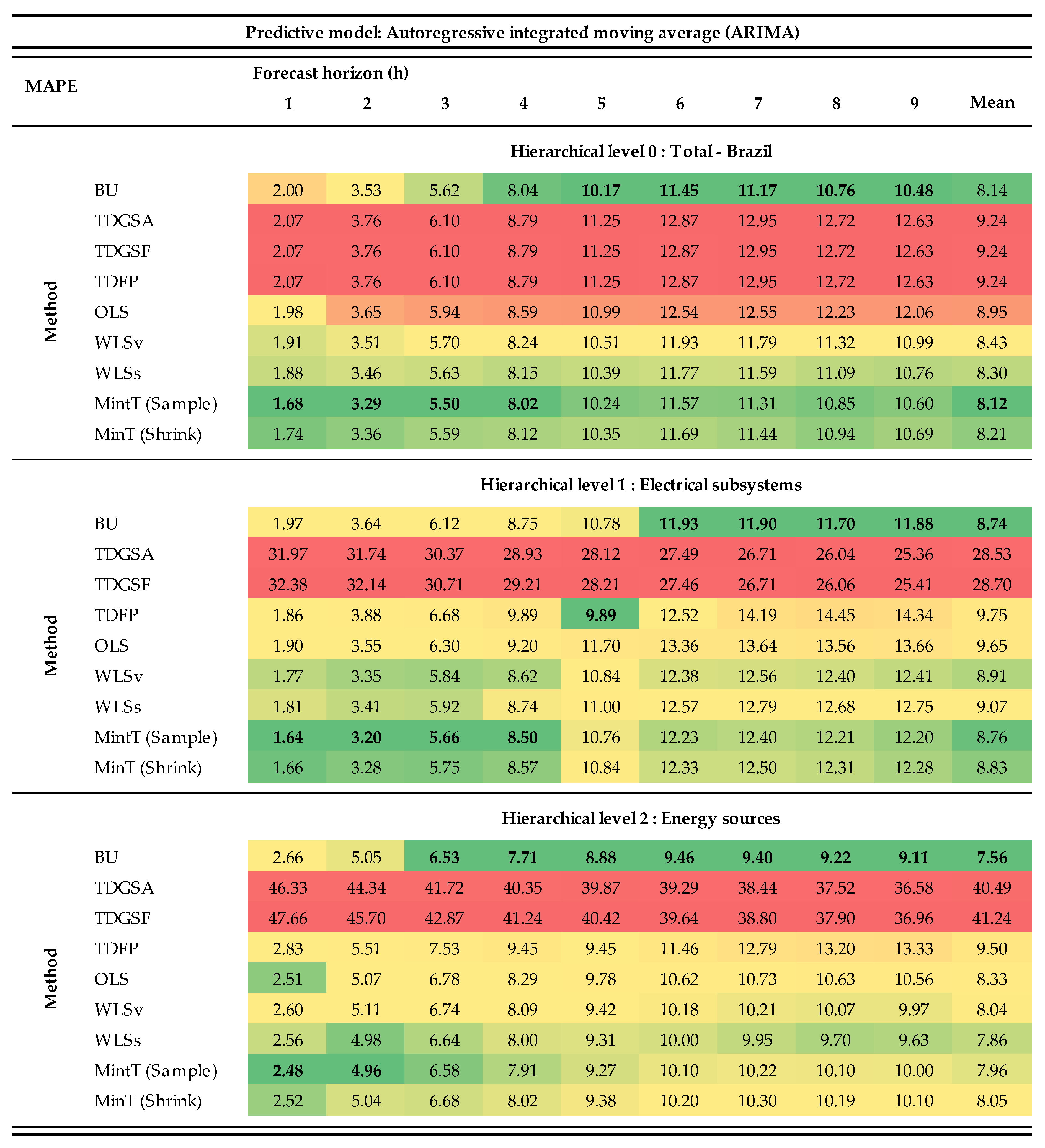
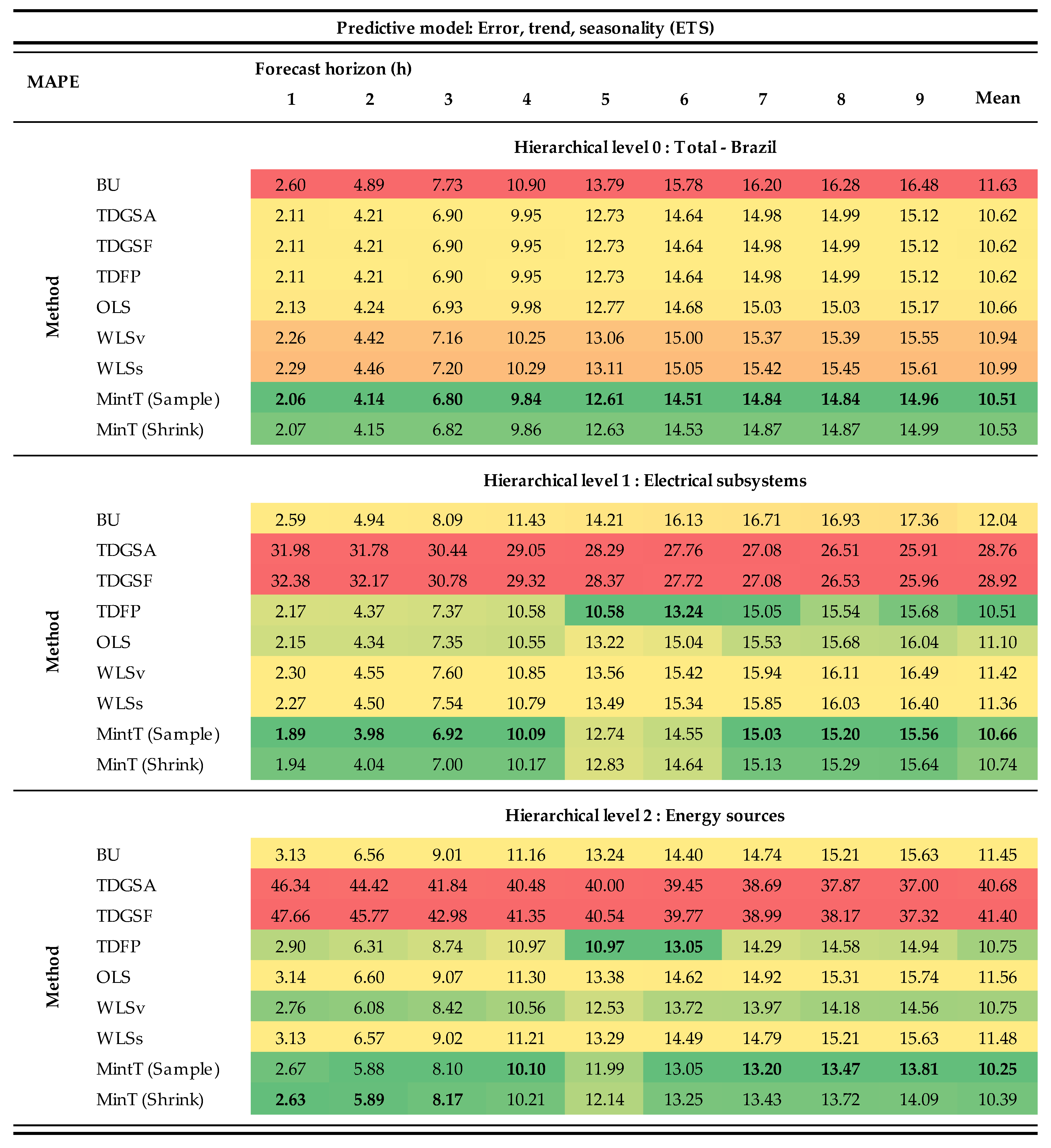
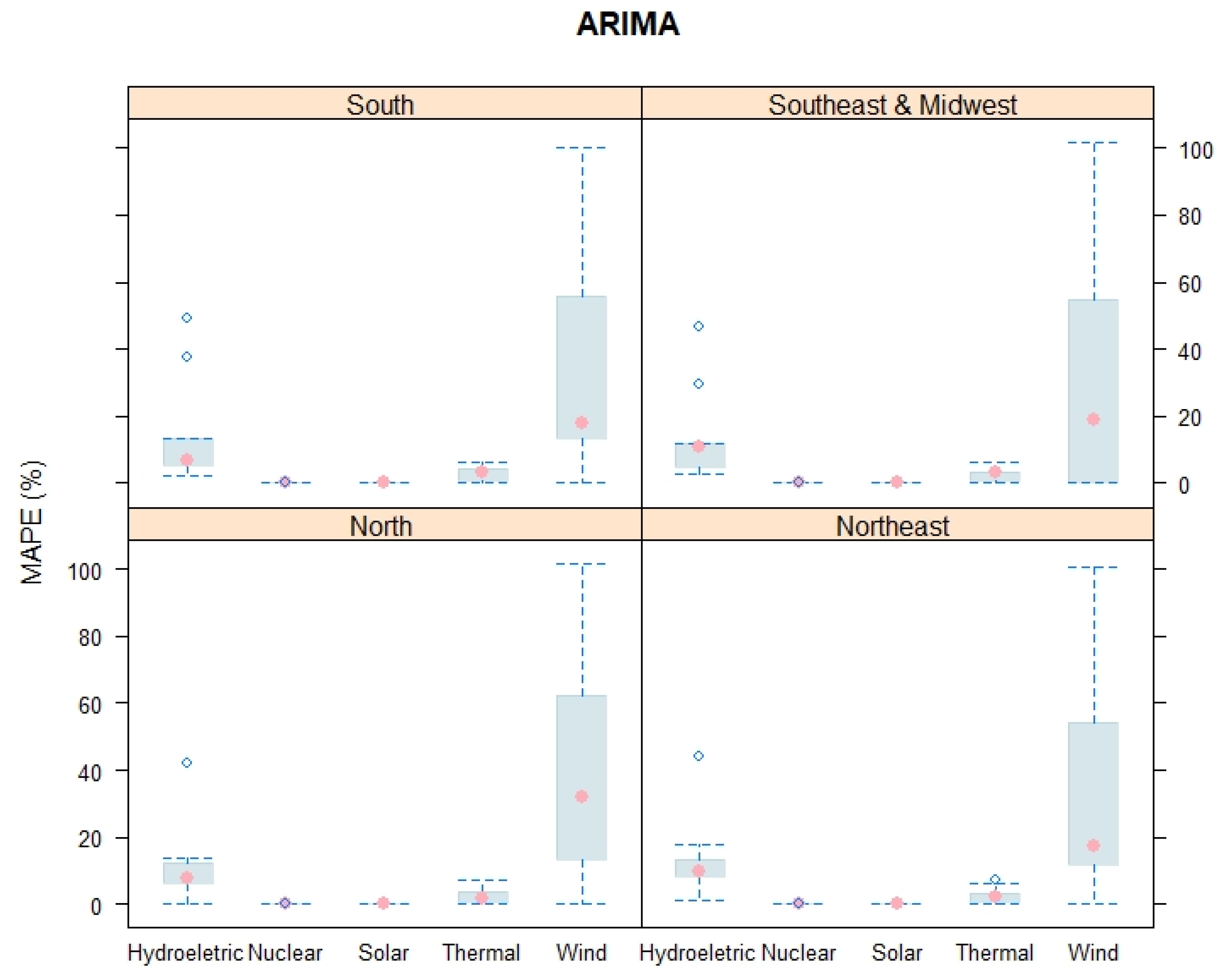
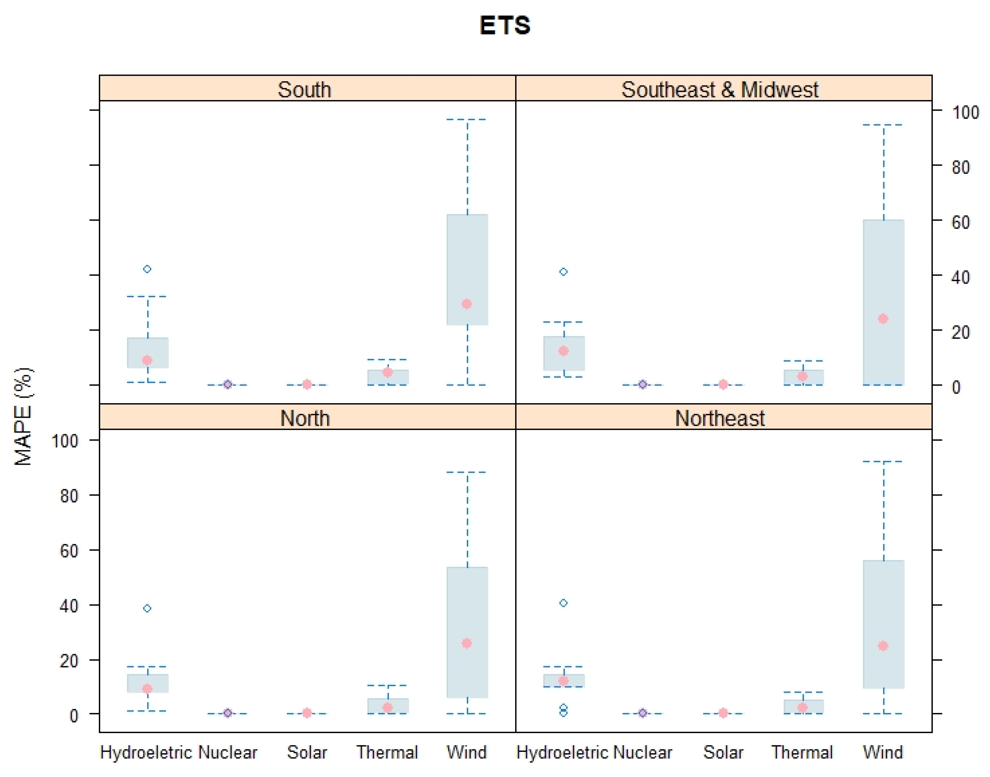
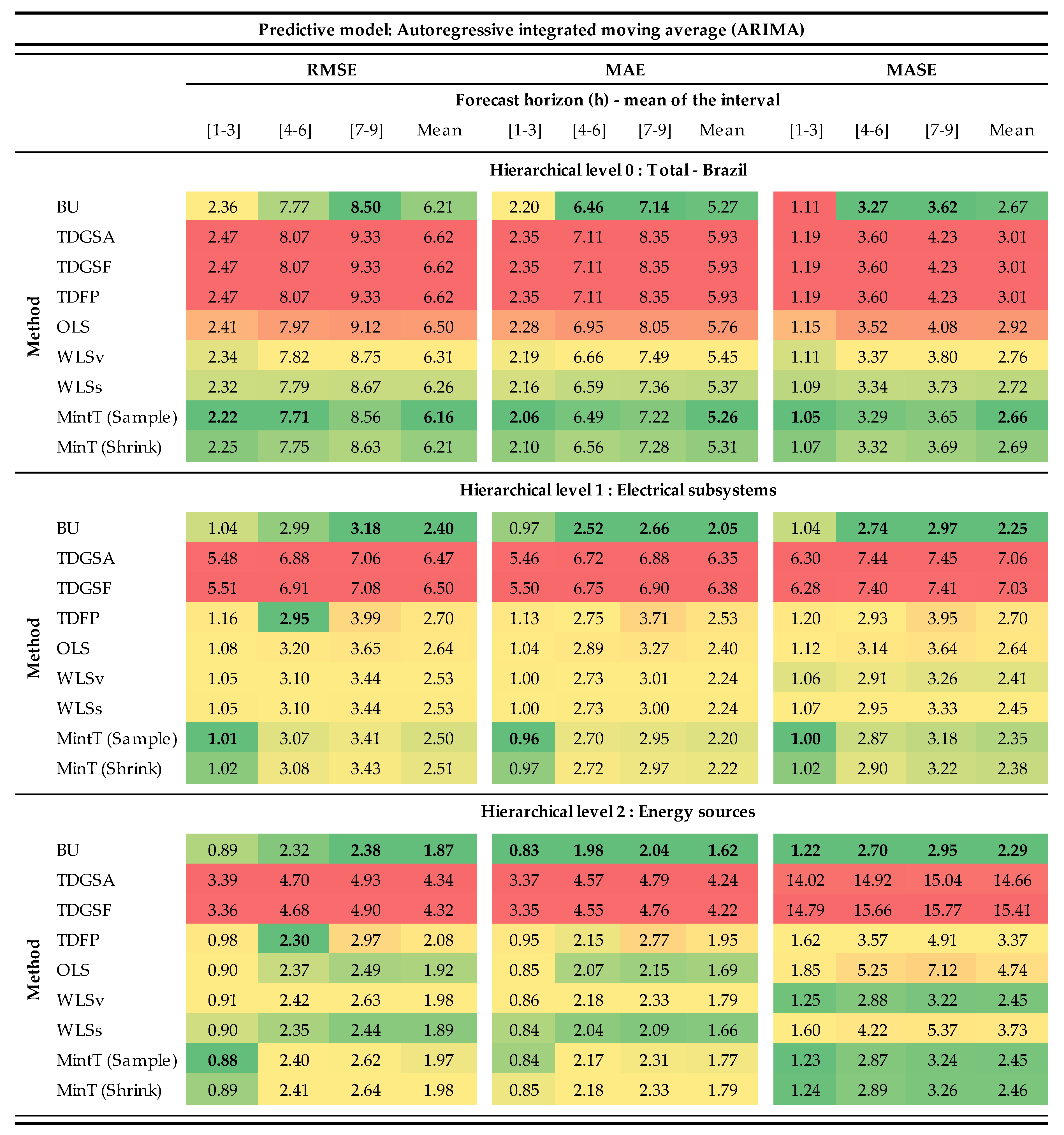
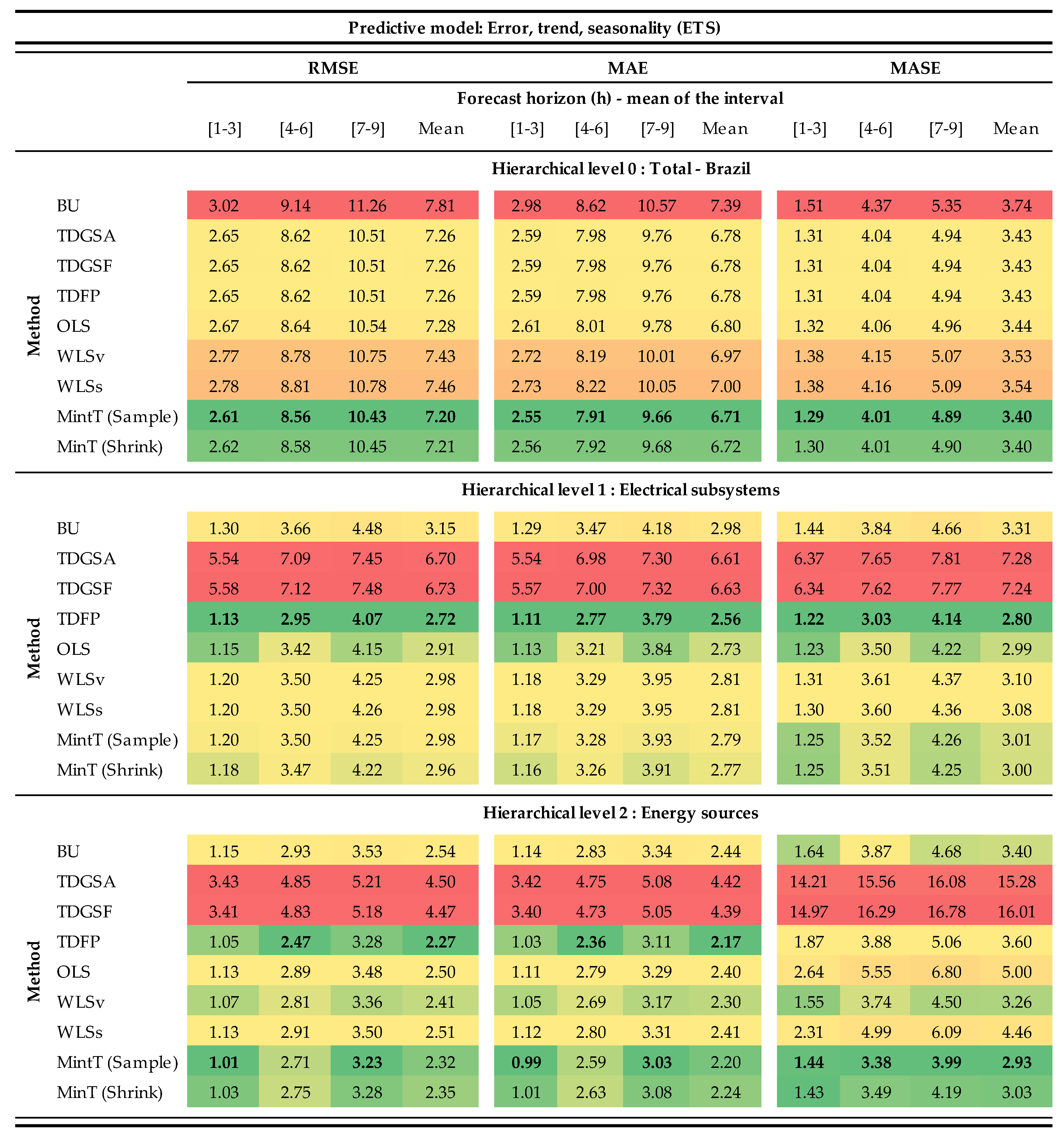
3. Results and Discussion

Figure 2, below, shows the predictive result obtained, using the ARIMA model, considering a predictive window of nine hours $(h=1,\dots ,9)$. Note that the model was estimated, taking the main hierarchical adjustment approaches into account, for the following levels: (i) total power generation in Brazil (Level 0), (ii) total energy generation by electrical subsystem (Level 1), and (iii) total energy generation by the energy generating source (Level 2). For Level 1, four forecasts (one for each electrical subsystem) were estimated. For Level 2, 14 forecasts (one for each energy source) were estimated.

Therefore, we estimated 1539 predictive models satisfying the following proportions: (i) 81 models for Level 0, (ii) 324 models for Level 1, and (iii) 1134 models for Level 2. The MAPE calculation for Levels 1 and 2 was based on a weighted average of the predictive errors. The weighting factors used are shown in Table 1.

The performance of each predictive model, divided by the forecast horizon, is illustrated by a color scale. The green colors indicate the most accurate forecasts, while the red colors symbolize less accurate forecasts. The best forecasts, for each of the predictive horizons, are highlighted in bold. The last column of Table 1 presents the average performance for each forecast horizon (h) for each hierarchical approach.

As pointed by [27], the MinT procedure has a useful feature: it systematizes results into a unique analytical solution that incorporates information about the correlation structure of the entire dataset. Additionally, the minimum trace reconciliation, with or without regularization, presented the best results of all linear reconciliation methods, such as OLS and WLS, with variations. Moreover, the MinT (Sample) approach returns the most accurate, coherent forecasts for all levels considering just the first forecast horizons. However, as the predictive window grows, the BU method becomes more accurate. Furthermore, the performance of the BU model increases as the time series disaggregate.

As expected, the results obtained using the top-down technique did not present good predictive results, since it is intended to generate forecasts for level 0, with worse accuracy for the other levels. Both BU and TD present disadvantages: they do not take the correlation among the series at each level into account.

The other accuracy metrics presented in the Appendix A (MAE, MAE, and RMSE) reinforce the results found. In general, the performance of the optimal reconciliation models, by trace minimization, provides more uniform estimates and better predictive potential for the first hours of the predictive horizon (Figure A3 and Figure A4).

In addition to the ARIMA predictive model, Figure 3 presents the same forecasting procedures. However, they are based on the ETS automatic adjustment model. The objective is to show the influence of different forecasting methods for each hierarchical reconciliation model. In general, the error percentage produced by the ETS model was slightly higher than that produced by the ARIMA model. Figure 3 also shows the influence of trace minimization procedures (MinT) on the improvement of predictive performance. In particular, the MinT models have good predictive performance, even with the increase of the forecast horizon hours.

The average performance of the trace minimization (MinT) models shows stability, considering all hierarchical levels. As shown in Figure 2, the ETS-based predictive model shares some similarities with the ARIMA model. The BU technique is better for the most disaggregated levels, whereas the TD technique stands out only at the more aggregated levels. Note that the trace minimization procedures show significant gains over the classic linear models, namely OLS and WLS.

Figure 2 and Figure 3 present some limitations. In general, it is not possible to test the predictive influence of each of the subsystems within the established forecast horizon. To show this problem, Figure 4 presents a predictive comparison (MAPE) for each of the Brazilian electrical subsystems, considering the nine-hour predictive horizon. On the left is the technique with the best aggregation/disaggregation performance (BU) for the ARIMA model. On the right is the technique with the best average performance (MinT) for the ETS automatic selection model.

Figure 4 thus shows a negative influence of the “south” electrical subsystem in the global measures of accuracy, especially from a predictive horizon of three hours onward. This system should be analyzed more thoroughly to identify energy sources located in the “south” subsystem that contributed most to the predictive instability of this system. Simultaneously, the use of individualized predictive models for this “south” system can be a good strategy, since unique climatic conditions exist in southern Brazil.

Figure A1 and Figure A2 (Appendix A) present the accuracy measure of the ARIMA and ETS models in detail, considering energy sources versus electrical subsystems. These results reinforce those in Figure 4, indicating instability in the southern subsystem, especially wind energy data.

Finally, some limitations of the present paper are recognized here. First, predictive models are based on past information evaluable, so the presented results cannot be extrapolated for different contexts and other time periods. Additionally, it is necessary to incorporate other predictive models to make the results more robust. In future research, it is recommended that models which integrate high-frequency data, e.g., the Wavelet approach, be adopted.

4. Conclusions

Analysis of the energy market is complicated. It involves the relationship between forecasting models and uncertainty, distinctly regarding the stochastic behavior of variables. The present paper is aimed at policymakers, offering a forecasting tool that deals with grouped time series. It also proposes a new forecasting approach, based on hierarchical modeling of the energy generation in Brazil.

The present paper introduces the use of trace minimization procedures (MinT) to aggregate and disaggregate forecasts based on the ARIMA and ETS models. MinT models performed better than the classic linear approaches, such as OLS and WLS. The MinT models also have high reliability for short predictive horizons. It is noteworthy that both hierarchical procedures and forecasting methods influence the predictive values of power generation in Brazil. Despite its advantages, the optimal reconciliation approach also has some limitations. This method could be unduly influenced by the sample period, and thus its ranking might change for other periods.

Therefore, the use of other predictive models, such as those based on analogs, machine learning, and other hybrid techniques, for example, is recommended. For future research, fine-tuning forecasts of the “south” electrical subsystem, as well as testing the accuracy of the hierarchal methods by using new forecasting approaches, is also recommended.

Finally, the present study contributes to the energy planning processes of different agents, given that understanding energy generation patterns is singularly important for minimizing risks and supporting reliable production planning. Good forecasts for future energy generation can support operational arrangements since energy supply and demand impact spot market sales prices.

References

1. Medojevic, M.; Medic, N.; Marjanovic, U.; Lalic, B.; Majstorovic, V. Exploring the impact of industry 4.0 concepts on energy and environmental management systems: Evidence from Serbian manufacturing companies. In Proceedings of the IFIP International Conference on Advances in Production Management Systems, Austin, TX, USA, 1–5 September 2019; pp. 355–362. [Google Scholar]
2. Alcácer, V.; Cruz-Machado, V. Scanning the industry 4.0: A literature review on technologies for manufacturing systems. Eng. Sci. Technol. Int. J. 2019, 22, 899–919. [Google Scholar] [CrossRef]
3. Bourdeau, M.; Zhai, X.Q.; Nefzaoui, E.; Guo, X.; Chatellier, P. Modeling and forecasting building energy consumption: A review of data-driven techniques. Sustain. Cities Soc. 2019, 48, 101533. [Google Scholar] [CrossRef]
4. Hammad, M.A.; Jereb, B.; Rosi, B.; Dragan, D. Methods and models for electric load forecasting: A comprehensive review. Logist. Sustain. Transp. 2020, 11, 51–76. [Google Scholar] [CrossRef] [Green Version]
5. Runge, J.; Zmeureanu, R. Forecasting energy use in buildings using artificial neural networks: A review. Energies 2019, 12, 3254. [Google Scholar] [CrossRef] [Green Version]
6. Choi, Y.B. Paradigms and Conventions: Uncertainty, Decision Making, and Entrepreneurship; University of Michigan Press: Ann Arbor, MI, USA, 1993. [Google Scholar]
7. Jiang, W.; Yan, Z.; Feng, D.H.; Hu, Z. Wind speed forecasting using autoregressive moving average/generalized autoregressive conditional heteroscedasticity model. Eur. Trans. Electr. Power 2012, 22, 662–673. [Google Scholar] [CrossRef]
8. Hao, C.H.E.N. A new method of load forecasting based on generalized autoregressive conditional heteroscedasticity model. Autom. Electr. Power Syst. 2007, 15, 012. [Google Scholar]
9. Stefenon, S.F.; Ribeiro, M.H.D.M.; Nied, A.; Mariani, V.C.; dos Santos Coelho, L.; da Rocha, D.F.M.; Grebogif, R.B.; de Barros Ruano, A.E. Wavelet group method of data handling for fault prediction in electrical power insulators. Int. J. Electr. Power Energy Syst. 2020, 123, 106269. [Google Scholar] [CrossRef]
10. Frizzo Stefenon, S.; Silva, M.C.; Bertol, D.W.; Meyer, L.H.; Nied, A. Fault diagnosis of insulators from ultrasound detection using neural networks. J. Intell. Fuzzy Syst. 2019, 37, 6655–6664. [Google Scholar] [CrossRef]
11. Gupta, S.; Srinivasan, D.; Reindl, T. Forecasting solar and wind data using dynamic neural network architectures for a micro-grid ensemble. In Proceedings of the 2013 IEEE Computational Intelligence Applications in Smart Grid (CIASG), Singapore, 16–19 April 2013; IEEE: New York, NY, USA, 2013; pp. 87–92. [Google Scholar]
12. Frizzo Stefenon, S.; Zanetti Freire, R.; dos Santos Coelho, L.; Meyer, L.H.; Bartnik Grebogi, R.; Gouvêa Buratto, W.; Nied, A. Electrical insulator fault forecasting based on a wavelet neuro-fuzzy system. Energies 2020, 13, 484. [Google Scholar] [CrossRef] [Green Version]
13. Moghaddam, A.A.; Seifi, A.R. Study of forecasting renewable energies in smart grids using linear predictive filters and neural networks. IET Renew. Power Gener. 2011, 5, 470–480. [Google Scholar] [CrossRef] [Green Version]
14. Barbounis, T.G.; Theocharis, J.B. A locally recurrent fuzzy neural network with application to the wind speed prediction using spatial correlation. Neurocomputing 2007, 70, 1525–1542. [Google Scholar] [CrossRef]
15. Xia, J.; Zhao, P.; Dai, Y. Neuro-fuzzy networks for short-term wind power forecasting. In Proceedings of the 2010 International Conference on Power System Technology, Hangzhou, China, 24–28 October 2010; IEEE: New York, NY, USA, 2010; pp. 1–5. [Google Scholar]
16. Dawan, P.; Sriprapha, K.; Kittisontirak, S.; Boonraksa, T.; Junhuathon, N.; Titiroongruang, W.; Niemcharoen, S. Comparison of power output forecasting on the photovoltaic system using adaptive neuro-fuzzy inference systems and particle swarm optimization-artificial neural network model. Energies 2020, 13, 351. [Google Scholar] [CrossRef] [Green Version]
17. Hyndman, R.J.; Kandahar, Y. Automatic time series forecasting: The forecast package for R. J. Stat. Softw. 2008, 26, 1–22. [Google Scholar]
18. Athanasopoulos, G.; Ahmed, R.A.; Hyndman, R.J. Hierarchical forecasts for Australian domestic tourism. Int. J. Forecast. 2009, 25, 146–166. [Google Scholar] [CrossRef] [Green Version]
19. Hyndman, R.J.; Ahmed, R.A.; Athanasopoulos, G.; Shang, H.L. Optimal combination forecasts for hierarchical time series. Comput. Stat. Data Anal. 2011, 55, 2579–2589. [Google Scholar] [CrossRef] [Green Version]
20. Almeida, V.; Ribeiro, R.; Gama, J. Hierarchical time series forecast in electrical grids. In Information Science and Applications (ICISA); Springer: Singapore, 2016; pp. 995–1005. [Google Scholar]
21. Panamtash, H.; Zhou, Q. Coherent probabilistic solar power forecasting. In Proceedings of the 2018 IEEE International Conference on Probabilistic Methods Applied to Power Systems (PMAPS), Boise, ID, USA, 24–28 June 2018; IEEE: New York, NY, USA, 2018; pp. 1–6. [Google Scholar]
22. Abouarghoub, W.; Nomikos, N.K.; Petropoulos, F. On reconciling macro and micro energy transport forecasts for strategic decision making in the tanker industry. Transp. Res. Part E Logist. Transp. Rev. 2018, 113, 225–238. [Google Scholar] [CrossRef]
23. Auder, B.; Cugliari, J.; Goude, Y.; Poggi, J.M. Scalable clustering of individual electrical curves for profiling and bottom-up forecasting. Energies 2018, 11, 1893. [Google Scholar] [CrossRef] [Green Version]
24. Silva, F.L.; Souza, R.C.; Oliveira, F.L.C.; Lourenco, P.M.; Calili, R.F. A bottom-up methodology for long term electricity consumption forecasting of an industrial sector-Application to pulp and paper sector in Brazil. Energy 2018, 144, 1107–1118. [Google Scholar] [CrossRef]
25. Ghedamsi, R.; Settou, N.; Gouareh, A.; Khamouli, A.; Saifi, N.; Recioui, B.; Dokkar, B. Modeling and forecasting energy consumption for residential buildings in Algeria using bottom-up approach. Energy Build. 2016, 121, 309–317. [Google Scholar] [CrossRef]
26. Kosiorowski, D.; Mielczarek, D.; Rydlewski, J. Forecasting of a hierarchical functional time series on example of macromodel for day and night air pollution in silesia region: A critical overview. arXiv 2017, arXiv:1712.03797. [Google Scholar]
27. Wickramasuriya, S.L.; Athanasopoulos, G.; Hyndman, R.J. Optimal forecast reconciliation for hierarchical and grouped time series through trace minimization. J. Am. Stat. Assoc. 2019, 114, 804–819. [Google Scholar] [CrossRef]
28. National System Operator. Operation History (Report of Power Generation). 2020. Available online: http://www.ons.org.br/paginas/resultados-da-operacao/historico-da-operacao (accessed on 15 May 2020).
29. R Core Team. R: A Language and Environment for Statistical Computing; R Foundation for Statistical Computing: Vienna, Austria, 2020; Available online: https://www.R-project.org/ (accessed on 15 May 2020).
30. Orcutt, G.H.; Watts, H.W.; Edwards, J.B. Data aggregation and information loss. Am. Econ. Rev. 1968, 58, 773–787. [Google Scholar]
31. Gross, C.W.; Sohl, J.E. Disaggregation methods to expedite product line forecasting. J. Forecast. 1990, 9, 233–254. [Google Scholar] [CrossRef]
32. Oliveira, J.M.; Ramos, P. Assessing the performance of hierarchical forecasting methods on the retail sector. Entropy 2019, 21, 436. [Google Scholar] [CrossRef] [Green Version]
33. Yang, D.; Kleissl, J.; Gueymard, C.A.; Pedro, H.T.; Coimbra, C.F. History and trends in solar irradiance and PV power forecasting: A preliminary assessment and review using text mining. Sol. Energy 2018, 168, 60–101. [Google Scholar] [CrossRef]
34. Panigrahi, S.; Behera, H.S. A hybrid ETS–ANN model for time series forecasting. Eng. Appl. Artif. Intell. 2017, 66, 49–59. [Google Scholar] [CrossRef]
35. Dong, Z.; Yang, D.; Reindl, T.; Walsh, W.M. Short-term solar irradiance forecasting using exponential smoothing state space model. Energy 2013, 55, 1104–1113. [Google Scholar] [CrossRef]
36. Box, G.E. Jenkins. In Time Series Analysis: Forecasting and Control; Holden-Day Inc.: New York, NY, USA, 1976. [Google Scholar]
37. Pegels, C.C. Exponential forecasting: Some new variations. Manag. Sci. 1969, 311–315. [Google Scholar]
38. Gardner, E.S., Jr. Exponential smoothing: The state of the art. J. Forecast. 1985, 4, 1–28. [Google Scholar] [CrossRef]
39. Hyndman, R.J.; Koehler, A.B.; Snyder, R.D.; Grose, S. A state space framework for automatic forecasting using exponential smoothing methods. Int. J. Forecast. 2002, 18, 439–454. [Google Scholar] [CrossRef] [Green Version]
40. Taylor, J.W. Exponential smoothing with a damped multiplicative trend. Int. J. Forecast. 2003, 19, 715–725. [Google Scholar] [CrossRef] [Green Version]
41. Liu, Z.; Yan, Y.; Yang, J.; Hauskrecht, M. Missing value estimation for hierarchical time series: A study of hierarchical Web traffic. In Proceedings of the 2015 IEEE International Conference on Data Mining, Atlantic City, NJ, USA, 14–17 November 2015; IEEE: New York, NY, USA, 2015; pp. 895–900. [Google Scholar]
42. Weiss, C. Essays in Hierarchical Time Series Forecasting and Forecast Combination. Ph.D. Thesis, University of Cambridge, Cambridge, UK, 2018. [Google Scholar]
43. Hong, T.; Xie, J.; Black, J. Global energy forecasting competition 2017: Hierarchical probabilistic load forecasting. Int. J. Forecast. 2019, 35, 1389–1399. [Google Scholar] [CrossRef]
Figure 1. Hierarchical aggregation structure for the energy generation in Brazil.
Energies 13 03722 g001
Figure 2. Hierarchical forecasting for electricity generation based on the ARIMA procedure (MAPE). (Note: The performance was indicated into a color scale, where green means better values for calculated accuracy, and red means worse accuracy. The intermediate values are colored yellow.).
Energies 13 03722 g002
Figure 3. Hierarchical forecasting for electricity generation based on the ETS procedure. (Note: The performance was indicated into a color scale, where green means better values for calculated accuracy, and red means worse accuracy. The intermediate values are colored yellow.).
Energies 13 03722 g003
Figure 4. Hierarchical forecasting for power generation: electrical subsystem versus forecast horizon.
Energies 13 03722 g004