Abstract
The Hydrothermal Coordination problem consists of determining an operation policy for hydroelectric and thermoelectric plants within a given planning horizon. In systems with a predominance of hydraulic generation, the operation policy to be adopted should specify the operation of hydroelectric plants, so that hydroelectric resources are used economically and reliably. This work proposes the implementation of reservoir operation rules, using inter-basin water transfer through an optimization model based on Network Flow and Particle Swarm Optimization (PSO). The proposed algorithm aims to obtain an optimized operation policy of power generation reservoirs and consequently to maximize the hydroelectric benefits of the hydrothermal generation system, to reduce the use of thermoelectric plants, the importation and/or energy deficit and to reduce the cost associated with meeting the demand and reduce CO2 emissions from combustion of fossil fuels used by thermoelectric plants. In order to illustrate the efficiency and effectiveness of the proposed approach, it was evaluated by optimizing two case studies using a system with four hydroelectric plants. The first case study does not consider transfer and water and the second case study uses water transfer between rivers. The obtained results illustrate that the proposed model allowed to maximize the hydroelectric resources of a hydrothermal generation system with economy and reliability.
1. Introduction
In recent decades, sustainable development has been a major concern for both developed and emerging countries [1]. The strong participation of renewable energy sources in a country’s energy matrix can promote an increase in sustainable development, given that economic growth is strongly associated with energy use [2].
Electricity is an essential resource for modern society and represents a catalyst for the economic development of a country [3]. Brazil is considered a country with continental dimensions and stands out for having a predominantly renewable electric matrix [4], with emphasis on hydraulic generation that acts with 66.6% of the domestic supply. Renewable energy sources correspond to 83.3% of the Brazilian electricity supply, which is the result of the sum of the amounts referring to national production plus imports, which are essentially of renewable origin, according to the 2019 National Energy Balance (NEB), base year 2018 [5]. In addition, according to NEB [5], in 2019 the internal supply of energy derived from thermoelectric plants corresponded to 26.7% of the electric power generation in the country. Such information allows us to characterize the country’s energy supply system as a hydrothermal generation system.
In addition, according to NEB, the country’s installed capacity in 2018 increased from 157,112 MW to 162,840 MW due to the expansion of hydro, solar and wind power generation with percentages referring to the increase of 2.30%, 400% and 11.76%, respectively. These data confirm the country’s commitment to the expansion of the electricity sector through the use of renewable energy sources, helping to promote Brazil’s economic growth in a sustainable manner.
For the efficient and effective supply of electricity, as important as the expansion and diversification of the energy matrix, it is essential to conduct studies regarding the behavior of the hydrothermal system. Therefore, different hydrological scenarios are used, with different sets of power plants in order to meet a certain demand. Such studies aim to minimize the costs related to the dispatch of the hydrothermal system, as well as to optimize the available electric resources. In addition, these studies can also contribute to the management, prevention and minimization of negative environmental and social impacts arising from the electric power production, a fact that represents a technological challenge for any nation.
Sustainable development is based on the economic, social and environmental pillars. A country wishing to develop a system considered sustainable must consider all three pillars. Electricity is fundamental for economic and social development, but it is well known that the energy sector is one of the main responsible for environmental pollution, especially for the use of thermoelectric plants [6,7]. Thus, the generation of clean electricity by minimizing the use of fossil fuel plants can contribute to sustainable development [8].
The Hydrothermal Coordination problem consists in determining an operation policy for hydroelectric and thermoelectric plants within a given planning horizon. In Brazil, where the predominance of electric power generation comes from hydroelectric plants, hydrothermal coordination aims to replace, as much as possible, high-cost thermal generation by hydroelectric generation, with practically zero cost, in a rational manner [9,10,11]. In this sense, the aim of hydrothermal coordination is to find an operational policy of reservoirs of hydroelectric plants that satisfies the energy requirements and system demand, in an economical and reliable way. Therefore, the optimal generation targets of each plant should be determined at each interval of the planning horizon to meet the demand reliably in order to minimize the expected cost of hydrothermal system operation over the entire planning horizon [11,12,13,14].
From the economic view point of hydrothermal coordination, to balance the compromise between the benefit of present water use for hydroelectric generation is sought, replacing rationally the thermoelectric generation as far as possible, and the expected future benefit, resulting from its storage, measured in terms of fuel economy [15,16,17,18].
The rational use of hydroelectricity brings a number of advantages, as this generation source not only provides a stable energy supply but can also supply peak moments [19,20], it may also be complemented by the growing sources of generation in Brazil such as wind energy [21,22] and solar photovoltaic [23,24,25,26]. In addition, hydroelectricity production can be started or stopped quickly by turning turbines on or off, allowing them to meet changing demand over time [19,20]. In addition to these advantages, we can mention the non-use of fossil fuels, avoiding the emission of CO2 into the atmosphere, the use of reservoirs for tourism and recreation and the clean energy production, without polluting rivers and affluents.
The problem of hydrothermal coordination is classified as a large problem due to the large number of plants, in which each has a large number of variables involved. It is also characterized as spatially-coupled due to the fact that the system plants are highly interconnected both hydraulically and electrically. It is also considered a time-coupled problem, as decisions made in a given planning period are dependent on past decisions and influence the future evolution of the system. In addition, some equations for calculating the hydroelectric and thermoelectric generation of the system are nonlinear, as well as the objective function of the system, characterizing the problem as nonlinear. Finally, the randomness of natural flows, together with the uncertainty of demand, makes the problem essentially stochastic [27,28,29].
The approach used in the problem of hydrothermal coordination is strongly influenced by the characteristics of each system, such as the prevalence or not of hydraulic generation, the representation of the system, the consideration or interconnection restrictions, among other factors. Therefore, different approaches are used to solve the problem, maintaining the basic philosophy regarding its objectives to be achieved.
Of the optimization techniques worth mentioning: Linear Programming (LP): it is an optimization method that is easy to implement and that allows solving a series of problems, both linear and non-linear, considering the restrictions and the objective function of the problem to be optimized as linear functions. By using only linear functions, PL needs to linearize the hydraulic generation function and the cost function of thermoelectric plants, given that these functions are non-linear [30]. Nonlinear Programming (NLP): addresses a problem taking into account the objective function and restrictions as non-linear functions. The limitation of NLP is related to the lack of guarantee of convergence of the iterative processes involved in the solution techniques, or else, this convergence requires a very high computational time [31]. Stochastic Dynamic Programming (SDP): it consists of a sequential decision-making process, where an overall optimal decision can be obtained through the optimization of individual subproblems [32]. The main disadvantage of the SDP is the so-called “curse of dimensionality”, caused by the increase in the number of all possible solutions that can be generated in each state, resulting in exponential growth and high computational effort, making the solution of the problem unfeasible. Stochastic Dual Dynamic Programming (SDDP): it represents a variant of the SDP, was proposed by [33] and uses the equivalent energy reservoir system model in order to reduce the problem dimension and the computational cost of the algorithm, trying to get around the curse of dimensionality. Bioinspired metaheuristics: they represent a set of alternative techniques that have shown very promising results when applied to the problem of Hydrothermal Coordination. Of the bioinspired algorithms, the following stand out: Genetic Algorithms (GA) [34], Artificial Neural Networks (ANNs) [35], Ant Colony Optimization (ACO) [36], Fuzzy Inference Systems [28], Particle Swarm Optimization (PSO) [15], among others.
Regarding the use of inter-basin water transfer to optimize the Hydrothermal System, it is worth mentioning the work of Gramulia Junior [37] who solved the problem of hydrothermal coordination using a GA, using the final volume of the plant and the natural inflow as decision variables. Of the works applied with bioinspired heuristics, none of them guarantees the feasibility of the solutions produced during the execution of the algorithm.
This work proposes a nonlinear, deterministic optimization model based on Network Flow and Particle Swarm Optimization applied to the problem of hydrothermal coordination that uses inter-basin water transfer and individualized operation of hydroelectric plants The developed computational model is the result of the integration between an algorithm of Network Flow (NF) and a Particle Swarm Optimization (PSO) algorithm.
Water transfer can contribute to the best use of hydroenergetic resources by allowing the efficient use of hydroelectric plants that are underutilized by the low volume of water that reaches their reservoirs. The idea is that a donating plant can give part of the volume stored in its reservoir without major losses in the production of electricity to another plant, called receiving. This, in turn, would be responsible for providing a high energy gain caused by the increase of water granted by the donating plant, maximizing the generation of electricity. Such methodology may contribute to the reduction of the use of thermoelectric plants, reducing the operational cost of the hydrothermal systems, and may also help to reduce the emission of gases responsible for global warming, such as CO2, reducing the environmental impacts associated with the generation of electricity.
The implemented algorithm was tested using two case studies, considering different hydrological periods and different conditions of natural flow. In both studies, three cascade reservoir hydroelectric power plants and one run-of-river power plant with and without the use of transfer were used. The first one consisted of 03 hydroelectric plants in the cascade reservoir and one in a stream without the use of transfer; and the second one consisted of a system with the same plants, but using the inter-basin water transfer. Such approach aims to maximize hydroelectric benefits by presenting a low-cost operation policy of the Brazilian hydrothermal system capable of meeting the demand in an economical and reliable way.
The paper was divided into five sections: Section 2 aims to present the mathematical modeling of hydrothermal coordination using the individualized representation of hydroelectric plants. This section also presents the mathematical modeling used in the inter-basin water transfer; Section 3 shows the proposed approach for solving the problem of hydrothermal coordination with inter-basin water transfer. The developed algorithm is a combination of a Network Flow responsible for modeling the hydroelectric system and a Particle Swarm Algorithm responsible for the walk direction of the decision variables modeled in the problem; Section 4 presents the case studies analyzed in the work, the results found by each of them and the discussions about the results. Here, an analysis of the environmental impacts related to the use of inter-basin water transfer is also carried out to solve the problem of hydrothermal coordination; the conclusion of the paper is present in Section 5.
2. Mathematical Modeling
This section describes the mathematical formulation employed in the developed algorithm. It is divided into three subsections. The first subsection deals with the mathematical modeling of Hydrothermal Coordination; the second is about the modeling of water transfer between rivers and basins; the next subsection presents the optimized reservoir operation policy.
2.1. Mathematical Modeling of Hydrothermal Coordination
In summary, the mathematical modeling of the hydrothermal coordination problem with individualized representation of hydroelectric power plants and with deterministic inflows can be established as the minimization of the system operating cost over the entire planning horizon, given by:
s.a.
where:
- T: number of intervals of the planning horizon;
- N: number of hydroeletric plants;
- : coefficient of present value;
- : total complementary generation (thermal, energy import and deficit) (MW);
- : total hydroelectric generation (MW);
- : demand (eletric energy market) (MW);
- : volume stored in the reservoir i at the end of the interval t (hm);
- : specific productivity of plant i ();
- : average volume stored in the reservoir i at the end of the interval t ();
- : volume evaporated in the reservoir i in the interval t ();
- : net water head of the plant t in the interval t ();
- : incremental water inflow to the reservoir of the plant i in the interval t ();
- : turbinated flow of the plant i in the interval t (/s);
- : flow release of the plant i in the interval t ();
- : spill flow of the plant i during the interval t ();
- : minimum and maximum bounds of stored volume for the reservoir of the plant i at the end of interval t ();
- : minimum and maximum bounds of the flow realese for the plant i in the interval t ();
- : minimum and maximum bounds of turbinated flow for the plant i in the interval t ();
- : minimum and maximum bounds of hydraulic generation for the plant i in the interval t (MW);
- : number of seconds in the interval t in seconds ();
- : group of indexes of the plants immediately upstream of plant i;
The objective function in Equation (1) consists of two terms, representing the operating cost over the planning horizon (E) and future cost related to the future state of reservoirs of hydroelectric plants (). Equality (2) represents the constraint of meeting to demand on interval t. Equation (3) represents the hydraulic generation of plant i in the planning period t. Equation (4) represents the calculation of hydraulic generation for all hydroelectric power plants on interval t. The reservoir water balance in the interval t is represented by Equation (5). This constraint indicates that the final reservoir volume is equal to the initial volume, added to the input flow (incremental flow and flow release of the power plants immediately at upstream) subtracted from the output flow (flow release) and evaporated volume. Equality (6) represents the flow release in the interval t, which is the result of the sum of the turbinated flow and the spill flow. Inequalities (7), (8), (9) and (10) represent the bounds of the reservoir volumes, the flow release, the turbinated flow and the hydraulic generation of the plants in the interval t, respectively. Initial reservoir volumes are given in Equation (11). The calculation of the hydraulic generation of a plant i in a planning period t, given by Equation (3), depends on the net water head (). This variable is calculated by the difference between the water level in the reservoir, called the upstream level, and the level of the river downstream, called the downstream level minus the hydraulic head loss.
2.2. Mathematical Modeling of Water Transfer Applied to Hydrothermal Coordination
In order to be able to transfer inter-basin water to benefit hydroelectric power generation, some modifications to the mathematical formulation described in the previous section have been changed. Therefore, consider that a hydroelectric plant is considered a donor (DP) when it gives away part of the water stored in its reservoir for transfer; a plant is considered a receiver (RP) when it receives water transferred by the donating plant using it to maximize the production of electricity. The amount of water to be transferred from DP to RP to benefit the entire hydrothermal system was calculated by the optimization algorithm which will be described in more detail in the next section.
At the donor plant, the transfer draws water from the incremental water flow () at time t. Let amount of water to be transferred in in the interval t. The value of the new incremental natural flow, called the artificial incremental natural flow, is given by:
That is, in the planning interval t part of the incremental flow of plant i is removed to be donated to another plant. With the new value of the incremental flow of the plant, given by Equation (12), it is possible to recalculate the value of the flow release () of the donor plant using Equation (5), keeping the same values of the other variables of the equation.
The water taken from the incremental natural flow of donating plant, is transferred to the receiving plant and will be added to the flow release () of the plant. Therefore, considering Equation (5) again, it is possible to isolate the flow release, by obtaining the following equation:
After calculating the artificial incremental natural flow of the donating plant using Equation (12), the new flow release of the plant is calculated using Equation (13), replacing the incremental natural flow () with the artificial incremental natural flow (), using the following equation:
It is worth mentioning that this modification will reflect in all the plants of the cascade located downstream of the donating plant, being necessary to recalculate the decision variables of these plants. Details of this modification will be described in Section 3 of this paper.
For the receiving plant, the water transferred from the donating is injected directly into its flow release. In this case, the value of is added in Equation (13), obtaining Equation (15), as follows:
This way, the amount of water to be transferred will be calculated for each interval of the planning horizon. Such modification was made in an attempt to provide better use of hydroenergetic resources.
2.3. Optimized Operation of Hydroelectric Power Plant Reservoirs for Electric Power Generation
In hydroelectric systems, the operation policy seeks to specify the behavior of each hydroelectric plant to the system reservoir, respecting the spatial-coupling and time-coupling of the plants. The operation policy takes the amount of electricity produced by each plant, considering its individual characteristics, its position in the cascade and the storage condition of each reservoir [27].
The optimized operation of hydroelectric power plant reservoirs takes an initial set of volumes and flow releases and achieves a policy of managing hydraulic resources in such a way to avoid, as far as possible, the use of non-hydraulic supplementation over the entire planning horizon. This policy aims to minimize the cost of energy of the hydrothermal system and, consequently, to maximize the economic benefits of hydraulic generation.
This work sought to go beyond the development of an operating policy that would take into account the spatial-coupling of the plants. The proposed modeling also uses inter-basin water transfer in order to take advantage of the high productivity of plants that may be underused due to the low natural flow that reaches them. Thus, it is possible to make more efficient use of the hydroelectric benefits plants present in the Brazilian hydroelectric system, also allowing a reduction in the cost associated with the production of electricity for this system. It is also expected that through water transfer there will be a decrease in environmental impacts, mainly related to CO2 emissions, resulting from the use of thermoelectric power generation.
Figure 1 shows the decision variables used in the mathematical modeling of the hydrothermal coordination problem. Figure 1a shows the decision variables for a hydroelectric plant, the volume of the reservoir () and the flow release of the plant (). Figure 1b shows a cascade system with the variables of each hydroelectric plant. The variable represents the amount of water to be transferred from hydroelectric plant 1 to hydroelectric plant 4.

Figure 1.
(a) Decision variables used in the mathematical modeling of the Hydrothermal Coordination Problem; (b) Cascading Hydroelectric System representing the decision variables. The variable presented in (b) corresponds to the amount of water to be transferred from a donor plant to a recipient plant in time interval t.
3. Methodology
This section describes the methodology applied to the problem of hydrothermal coordination with the use of inter-basin water transfer. The Section 3.1 shows the network flow used in the modeling of the hydroelectric system; the Section 3.2 presents optimization model employed (PSO) and the last subsection shows the proposed approach (NF + PSO).
3.1. Network Flow Applied to Hydrothermal Coordination
The problem of Hydrothermal Coordination can be efficiently represented by a nonlinear network flow model with bounded arcs. Thus, for modeling the problem, each network node is considered as a hydroelectric power plant for a period of time. The arcs of network flow represents the volume stored in the reservoirs and the flow release of the plants in the planning period intervals. Therefore, in each node of the network only two arcs come out: one of flow release and one of volume. Figure 2 exemplifies the modeling using a system with 03 cascade reservoir hydroelectric power plants and the two arcs from each node.

Figure 2.
Hydrothermal Coordination modeling using Network Flow.
Each circle in the image represents a hydroelectric power plant in a interval of planning horizon. For example, circle 1,1 corresponds to plant 1 at time instant 1, circle 1,2 represents plant 1 at time instant 2. The horizontal black arrows represent the volume arcs corresponding to the temporal coupling of the plants. The spatial coupling is given by the red arrows corresponding to the flow releases from an upstream plant to a downstream plant. With this network flow modeling we can represent the water balance (Equation (5)) as the flow equilibrium equation of each node. The bounds imposed on the network arcs is represented by the constraints of the volume bounds and the flow of the plants. The use of the Network Flow based model enabled the guarantee the feasible solutions throughout the optimization process.
The Optimization methods that use network flow modeling use partitions of the total arc set between basic and nonbasic arcs. Basic arcs represent the dependent variables of the problem, while independent variables constitute the non-basic arcs [10,27,28]. The basic arc set forms a tree structure in the network. When a nonbasic arc is added to the network, a cycle is formed, where the orientation of the basic network arcs may agree or disagree with the formed cycle [10,29].
Optimization methods seek to determine a direction for the independent variables of the problem, aiming to improve the objective function response. For this work, the Particle Swarm Optimization (PSO) was used as to calculate the walking direction of the super basic arcs (independent variables) of the network flow. PSO details are described below.
3.2. Particle Swarm Optimization (PSO)
Particle Swarm Optimization is a search and optimization algorithm that simulates the social behavior of a flock of birds. In a basic PSO, individuals in a swarm, called particles, follow a very simple behavior: emulating the success of neighboring individuals and their own successes. The collective behavior that emerges from this simple strategy is that of finding optimal regions in a high dimensional search space [38,39,40].
The PSO algorithm maintains a swarm of particles that “fly” through a multidimensional search space. The position of each particle is adjusted according to its own experience and to its neighbors. Thus, let be the position of particle i in the search space at time t; where t represents a period of time. The position of the particle is changed by adding a velocity, , to the current position, that is:
In Equation (16), it is the velocity vector which drives the optimization process and reflects both the knowledge acquired by the particle and the information socially shared with the swarm. Acquired knowledge of a particle is generally referred to as the cognitive component, which is proportional to the particle’s distance from its own best position (referred to as the particle’s best personal position or pBest) found from the beginning of the optimization. Socially shared information is referred to as the social component of the speed equation (also referred to as the best swarm position or gBest). The particle velocity update is given by the following Equation (17):
where is the velocity of particle i in dimension at time t, is the position of particle i in dimension j at time t, and are the positive constants of acceleration used to dimension the contribution of the cognitive and social components, respectively and , are random values in the range . These random values introduce a stochastic element into the algorithm.
The best position associated with particle i, , is the best position the particle has visited since the first step. The best overall position, , at time step t, is defined as the best position discovered by any of the particles during any iteration.
3.3. Proposed Approach
This section describes the developed computational model based on Network Flow and PSO applied to the hydrothermal coordination problem. The inter-basin transfer between are also be discussed in this section.
3.3.1. Deployed Optimization Model (NF+PSO)
The developed algorithm is based on a PSO in which the problem modeling was performed by means of a Network Flow with capable arcs. The PSO acting as an optimizer has a number of advantages, including: easy implementation; it works with a population of solutions; it has few parameters to be adjusted; it does not require derivative calculation; and it is efficient for finding the global minimum/maximum as pointed out by [38,39,40,41,42]. The problem of Hydrothermal Coordination was modeled by a network flow, as this approach is commonly used in the literature mainly for exploring the special network structure of the problem as pointed out [10,27,28,29,43].
The proposed modeling aims to ensure the feasibility of the solutions produced throughout the process for the solutions, accompanied by an individualized representation of the hydroelectric plants, including important aspects such as the calculation of the maximum swallow as a function of the net fall height, the effect of backwater, quota effect, maximum/minimum limits of turbinated flow, flow realease, spill flow and volume, among others. Figure 3 summarizes the steps of NF+PSO.

Figure 3.
Proposed algorithm.
The algorithm is basically divided into 3 phases: phase I is responsible for generating the feasible initial swarm, i.e., for the initialization of the swarm particles. Phase II is responsible for the operation policy of the reservoirs of hydroelectric power plants, i.e., it is the stage that aims to calculate the volume and the flow release of each plant in each planning horizon. Phase (III) occurs simultaneously with phase II and aims to obtain the optimal values to be transferred from the donating plant to the receiving plant in each period of the planning horizon.
- Step 1—Particles Initialization: In this step the position and velocity of the particles are initialized. The position of a particle is represented by a two-dimensional matrix , where N corresponds to the number of hydroelectric power plants in the system and T corresponds to the number of intervals of the planning horizon. The matrix has columns, because the first T columns of the matrix represent the reservoir volume and the second half of the columns refers to the flow release of the plants. Figure 4 illustrates the modeling used for PSO particles implemented for a hydrothermal system consisting of three hydroelectric and four months. This step corresponds to phase I of the algorithm and it is responsible for generating the feasible initial population.
 Figure 4. Position of the particle in the Network Flow (NF) + Particle Swarm Optimization (PSO).
 - Step 2—Particles Evaluation: The hydrothermal coordination optimization aims at minimizing the operational cost of the system. Thus, Equation (1) was used as a function of swarm particle evaluation to minimize the cost of hydrothermal system operation. The particle evaluation in the current iteration is compared to the evaluation in the previous iteration and, if the value of the current evaluation is better than in the previous iteration, the position vector is updated, otherwise it is retained.
- Step 3—FindinggBest: In this phase, the search for the best particle is performed, that is, the one with the best suitability of the whole swarm for subsequent updating of the swarm particle velocity.
- Step 4—Network Flow part 01: The first step of Network Flow is responsible for determining the non-basic arcs named super basic, i.e., through the Arc Partition Strategies (APS), the Network Flow establishes for each particle, according to its position vector, which elements of this vector will be updated. The details of each APS are described below:
- -
- Step 4.1—Arc Partition Strategy based on Hydraulic Production Function (APS-HPF): This arc splitting strategy recommends that, as far as possible, the basic arcs be composed of volumes. Thus, if a volume arc is within its operating limits, this arc will be at the base. Otherwise, the basic arc will be a flow release arc. As a result that the process is iterative, if the volume arc falls within its limits during the next iterations, the volume arc returns to the base.
- -
- Step 4.2—Arc Partition Strategy based on Cascade Energy Transfer 1 (APS-CET1): This strategy attempts to transfer energy among all periods of the planning horizon, that is, it attempts to transfer energy across the entire cascade (power plants system) and among all planning intervals, allowing the transfer of large blocks of energy between intervals. Energy transfer is done by creating a cycle between two intervals, in which changes made by the PSO are made only on the variables in that cycle.
- -
- Step 4.3—Arc Partition Strategy based on Cascade Energy Transfer 2 (APS-CET2): This APS represents a variant of APS-CET1, in which the main difference is the transfer of energy only between the planning horizon periods defined between the intervals of highest and lowest marginal cost of system operation.
- Step 5—Particles Velocity Update: Since PSO works together with network flow, the update of the velocity performed by Equation (17) will only be applied at the velocity vector positions at which Network Flow defined as super basic arcs, calculated by step 4. Therefore, there is only the updating of the velocity vector positions related to the super basic arcs. This fact decreases the computational cost, since the entire velocity vector is not updated. In this step the PSO velocity updating is used to seek the walking direction of the super basic arcs.
- Step 6—Network Flow part 02: In the second phase of the network flow, the following steps are performed:
- -
- Step 6.1—Cycles Identification: A cycle occurs when a super basic arc is inserted into the tree structure of the net, in which the orientation of the net basic arcs may agree or disagree with the formed cycle, which is determined by the orientation of the inserted super basic arc. Modifying the arcs values of a cycle allows the calculation of the effect of this change on the objective function. Thus, after the identification of the super basic arcs in step 4 and the walking direction in step 5, in this step there is the identification of the cycles formed by the addition of the super basic arc in the tree structure. Figure 5 shows the cycle formed by the addition of the super basic arc in the tree structure defined by the basic arcs , forming the cycle , which are within the dashed area in red.
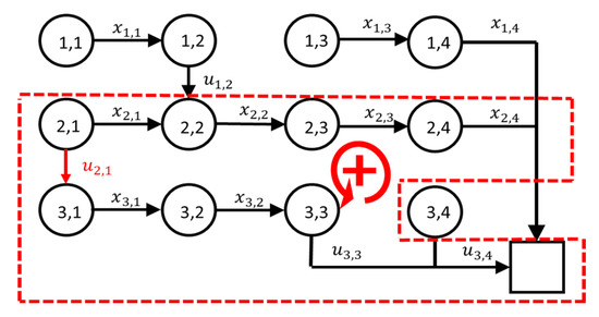 Figure 5. Cycle formed by addition of the arc .
 - -
- Step 6.2—Walk Projection of Super Basic Arcs: This step is intended to prevent the canalization violation of the super basic arcs. In order to prevent this, the walk direction of the super basic arch should be annulled when it is within one of its limits, and its walk direction would imply in a violation of your canalization. For instance: If the super basic arc is at its lower limit (minimum flow release) and the walk direction of this arc implies a decrease in its value, its walk direction should be zero so as to avoid a violation of its minimum canalization limit.
- -
- Step 6.3—Basic Arcs Walk Direction: The walk direction of basic arcs is calculated based on the cycles formed by the super basic arcs in which the basic arcs participate. For each cycle, the walk direction of the basic arcs refers to the values given by combining (sum) the directions of the super basic arcs, in which the base arcs that agree with the direction of the formed cycle will be positive, otherwise they will be negative. In the example in Figure 5, the base arcs agree with the super basic arc and the basic arcs disagree with .
- -
- Step 6.4—Maximum Step Calculation: The maximum step size is calculated so that none of the arcs violate their canalization limits. After calculating the walk direction of the super basic and basic arcs, the walk direction signal of the decision variable must be analyzed. Depending on the signal, negative or positive, the arc may vary to its lower or upper limit respectively. Therefore, for each decision variable, its maximum step is calculated, aiming at not violating its limits. The maximum step value for all decision variables is given by the smallest value found between the maximum steps of the variables that correspond to a basic arc or super basic arc present in at least one cycle.
- -
- Step 6.5 - Optimum Step Calculation: The optimal step value is determined by one-dimensional searching using the golden ratio method [44].
- Step 7—Particles Position Update: Since the velocity values of each position relating to the decision variables, defined by the network flow, are calculated, the position of the particle in the next iteration is updated by Equation (16). Thus, only the arcs of the cycle formed by the super basic arc are their values modified. Throughout the iterations of the algorithm, new cycles are formed updating the particles in search of the best operating policy for the hydrothermal system. Steps 2 through 7 correspond to optimization algorithm phase II and, therefore, they aim to find the optimal values for the final volumes and flow releases of each hydroelectric plant of the system.
- Step 8—Transfer Performance: This last step corresponds to phase III of the algorithm and it is responsible for calculating the optimal value to be transferred from the donating power plant to the receiving power plant based on the volume and flow release values of the current iteration. Thus, after each phase II iteration and based on the results found in this iteration, the corresponding phase III iteration begins. Details of this modeling will be described in the following subsection.
3.3.2. Optimization Model on Inter-basin Water Transfer
This step also are a network flow algorithm combined with a PSO that has all 07 steps of the algorithm of Figure 3 and all of them will be described below:
- Step 1—Particles Inicialization: In this step the position and velocity of the particles are initialized. The position of a particle is represented by a one-dimensional matrix T, where T corresponds to the number of intervals of the planning horizon. The matrix has T columns because, for each interval t, one must find the optimum value to be transferred from DP to RP. The Equation (18) presents the modeling of the particles used in Phase III of the algorithm, using a planning horizon with 6 intervals.
- Step 2—Particles Evaluation: The phase III aims to minimize the operational cost of hydrothermal system with the use of inter-basin water transfer. Therefore, Equation (1) was also used as evaluation function of swarm particle in order to minimize the cost of hydrothermal system operation. Differences from phase II to phase III are described in Section 2.2.
- Step 3—FindinggBest: In this phase, the search for the best particle of phase III is performed .
- Step 4—Network Flow part 01: This step is responsible for determining the non-basic arcs called phase III superbasic using the transfer arc partition strategy (APS-Transfer). This APS recommends that, as far as possible, the basic arc set be composed by volumes. Thus, if a volume arc is within its operating limits, this arc will be at the base. Otherwise, the basic arc will be a flow release arc. The super basic arcs will be the arcs that link the DP to the RP for all periods of the planning horizon. The APS-Transfer for a system consisting of 03 plants (the last one is a run-of-the-river power plant), and for a 4-intervals planning horizon is illustrated in Figure 6.
 Figure 6. The transfer arc partition strategy (APS-Transfer).
 - Step 5—Particles Velocity Update: This step aims to update the elements of the velocity vector at which the Network Flow has defined as super basic arcs (transfer arcs).
- Step 6—Network Flow part 02: As in phase II, in this one the following steps are performed:
- -
- Step 6.1—Cycles Identification: it identifies the cycle originated by the transfer arc. As in phase II, the orientation of the network basic arcs may or may not agree with the formed cycle. Figure 7 shows the cycle formed by the addition of the super basic arc in the tree structure defined by the basic arcs , forming the cycle .
 Figure 7. Cycle formed by addition of the arc .
 - -
- Step 6.2—Walk Projection of Super Basic Arcs: This phase is responsible for preventing violation of the canalization of the boundaries of the arcs involved in water transfer from both the donating plant and the receiving plant. Two such situations may occur: The first case is when the walk direction of the super basic arc implies a violation of the minimum volume of the donating plant, in which case more water is to be removed from the DP than it can provide. The second case occurs when the RP is already at its maximum flow release and cannot receive more water from the DP. Thus, if any of these situations should occur, the walk direction of the transfer arc super basic should be canceled, assigning the zero value to the super basic arc walking direction.
- -
- Steps 6.3, 6.4 and 6.5: These steps are performed in a similar way as they occur in phase II.
- Step 7—Particle Position Update: This step is responsible for updating the pTrans vector, which stores the positions related to the amount of water to be transferred from the donating plant to the receiving plant.
4. Results and Discussions
This section was dedicated to the study of water transfer between rivers and basins in order to contribute to the production of hydroelectricity, minimizing the cost of operating the hydrothermal power system. Therefore, the Barra Bonita, Promissão, Três Irmãos plants located on the Tietê river and the Henry Borden plant located on the Cubatão river were used. It should be noted that the Henry Borden plant is not interconnected with the other plants in the system. The studies presented in this section deserve attention, as the water transfer modeled in the algorithm will be used with this hydroelectric system, promoting the interconnection of the cascade composed by Barra Bonita, Promissão and Três Irmãos with the Henry Borden plant. In studies with water transfer, the Barra Bonita plant acted as the Donor plant and Henry Borden’s plant was the Receiver plant.
The Henry Borden complex, located in Serra do Mar, in the city of Cubatão, is composed of two plants called External and Underground. It has a drop height of 720 m and 14 groups of generators coupled with Pelton-type turbines. Henry Borden’s installed capacity is 889 MW, for a flow rate of 157 . As of October 1992, the operation of this system has been reduced by approximately 75%, to meet the conditions established by the Joint Resolution SMA / SES 03/1992, of 10/04/1992, updated by resolution SMA-SSE-02, of 02/19/2010, only allowing the pumping of the waters of the Pinheiros River to the Billings Reservoir for flood control [45].
The Henry Borden complex also stands out for its location, close to the largest consumer center of electricity in Brazil, contributing for more than 4 decades to the industrial development of the metropolitan region of São Paulo. Its location next to a large load center allows for shorter transmission lines, when compared to other hydroelectric plants, such as Belo Monte, for example, where shorter transmission lines are needed generating less losses. Second Gramulia Junior [37], its productivity of 5.65 is one of the largest in the plan, requiring approximately 157 to remain at full load. The Itaipu plant, for example, needs a flow 5.3 times greater to produce the same power.
In order to verify the correct functioning of the proposed algorithm with the new methodology, identifying the optimal amount of water to be transferred at each interval of the planning horizon, in order to minimize the cost of the system’s operation, two case studies were carried out with the four plants and the results are found in the following subsections. In all case studies was adopted the planning horizon with monthly discretization. May was considered the beginning of all planning horizons, given that this month shows the beginning of the dry period for the southeast system, region where the test system plants are located. The electricity demand was kept constant and equal to the installed capacity of the hydroelectric system (2100.5 MW). The two case studies are:
- Case Study 01: Test system using, as natural flows, 100% of the Long-Term Average (LTA) with and without transfer for a planning period of two years;
- Case Study 02: Test system using 100% of LTA the flow observed from May 2013 to April 2018 with and without water transfer.
The results as well as the discussions of each case study are presented in the following subsections.
4.1. Case Study 01
The first case study considers a two-year planning horizon, using 100% LTA as natural flow with and without transfer. The operative policy of the hydroelectric system with transfer are presented in the graph of the Figure 8.

Figure 8.
Volume trajectory of plants for 100% Long-Term Average (LTA) with water transfer.
From the graphs of Figure 8, it is possible to notice the variation of the reservoirs volume of the plants as a function of the position of the plant in cascade. The Barra Bonita plant, located further upstream, is responsible for regulating the natural flows, aiming to adjust the flow variation and prevent water spill. The Promissão plant, located in the intermediate position of the cascade, also has fluctuations in the volume of its reservoir, but more mildly, except between the months of 7 to 9 and 19 to 22. During the periods in which Promissão presented much more depletion, there was a large increase in the flow release, allowing such a plant to be able to empty its reservoir more sharply. Finally, the Três Irmãos plant is operated as its reservoir remaining at maximum volume for almost the entire planning horizon. This is due to cota effect [27,28]. This fact highlights that the energy stored in the system is valued by the productivity of the most downstream plants. Therefore, the Três Irmãos plant, besides being a plant with higher installed capacity, is operated with maximum productivity during most of the planning period. Thus, the proposed algorithm emphasized the filling of the downstream reservoirs to upstream ones and the depletion in the opposite direction. Henry Borden as run-of-the-river power plant, has no changes in the volume of his reservoir during the entire planning period.
The next figure shows the comparative graph of hydraulic generation with and without water transfer.
The graph in Figure 9 shows the difference in the amount of electricity produced by the system using the water transfer from Barra Bonita to Henry Borden. The average amount of water transferred was 151.99 . This result shows the great generation potential of Henry Borden hydroelectric power plant. Table 1 provides a comparison of the average electric power generation by each hydroelectric plant with and without transfer.
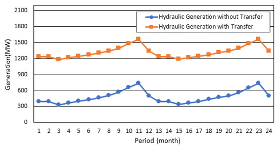
Figure 9.
Comparison of hydraulic generation with and without water transfer for case study 01.

Table 1.
Comparison of hydroelectric generation average with and without transference (average MW).
From the results found, it can be observed a generation increase of 716.96 MW with water transfer, representing a gain of 221.82% given by the great productivity of Henry Borden, 859.21 MW of electricity production with water transfer, on average.The hydroelectric plants of Barra Bonita, Promissão and Três Irmãos had a reduction in the production of electric energy of 27.19 MW, 32.79 MW and 61.74 MW, respectively. The sum of the generation reduction of the three plants represents a total of 121.72 MW, which corresponds to 14.16% of Henry Borden’s average production, showing the great efficiency of the proposed methodology.
4.2. Case Study 02
The second case study considers a five-year planning horizon and the natural flows used were 100% from May 2013 to April 2018. Figure 10 presents the operation policy for the case study with and without the use of water transfer.

Figure 10.
Volume trajectory of plants for case study 02 (2013-2018) with water transfer.
Even with the large flow irregularity, the system behavior for case study 02 is similar to case study 01. Therefore, Barra Bonita plant, because it is located further upstream, is responsible for controlling the accentuated seasonality of the natural flows for the period analyzed. Promissão also had variations in large part softer than Barra Bonita plant, except in months 31, 32 and 33, when it abruptly depleted its reservoir to preserve the high productivity of Três Irmãos. Três Irmãos plant operated for much of the planning period with maximum productivity. These results again highlight the influence of the cota effect.
Note that in the first year there was little depletion of all reservoirs in the system. This happened because in the interval between months 13 to 19 was the period when there was the lowest natural flow of the system. Therefore, in order to avoid the depletion of water, the hydroelectric plants have not depleted their reservoirs. Once again, Henry Borden, being a run-of-river power plant, had no change in volume throughout the planning horizon. The results found corroborate the results observed in the literature [10,16,27,28].
The graph in Figure 11 illustrates, again, the difference in the amount of electricity produced by the system using the water transfer from Barra Bonita to Henry Borden. Again, the amount of water transferred from Barra Bonita to Henry Borden had an average value of 151.99 . Table 2 provides a comparison of the average electric power generation by each hydroelectric power plant with and without transfer for case study 02.

Figure 11.
Comparison of hydraulic generation with and without transfer for case study 02.
Table 2.
Comparison of hydroelectric generation average of the system with and without transference fo case study 02 (average MW).
The results presented in Table 2 show, again, a significant increase in hydroelectricity production by water transfer from Barra Bonita to Henry Borden. The observed increase was 612.24 MW, representing an increase of 209.74%. Again, the Barra Bonita, Promissão and Três Irmãos plants had a 105.05 MW reduction in electricity production, representing a total of approximately 14.65% of Henry Borden’s production with water transfer.
In both case studies demonstrates the effectiveness of water transfer in relation to power generation of the hydroelectric system, significantly increasing the generation of hydroelectric power and decreasing the use of thermoelectric power and, consequently, the cost of operating the system and the resulting impacts from burning fossil fuels of energy production that is no longer generated by thermal power plants.
Results for the financial analysis of the electricity non-produced by Henry Borden and the Environmental Impacts resulting from the non-utilization of its maximum potential are presented in the next subsection.
The results presented in the two case studies demonstrate the feasibility of the proposal for optimization of the problem of Hydrothermal Coordination taking into account the inter-basin water transfer, identifying in all of them gains in hydroelectric energy production, confirming the relevance of the proposed methodology. Thus, the mathematical formulation presented for the water transfer allowed to find the necessary amount of water to be transferred in each interval of the planning period, optimizing the energy gains of the case system; the good results obtained in the application of the proposed optimization model showed the great potential of this tool, which managed to capture the different operating characteristics of the plants and inflows. It was observed that in the two case studies the algorithm that performs the water transfer presented a satisfactory performance in determining an operational strategy that will meet the restrictions of the Hydrothermal Coordination problem, ensuring the feasibility of all solutions during the process of system optimization.
4.3. Financial and Environmental Impact Analysis
Using the system presented in case study 02, it is possible to evaluate the financial value resulting from the unproduced electricity during this period, i.e., it was verified how much was not collected with the energy production from May 2013 until May 2018. Subsequently, it was analyzed the cost of this production of energy not generated by Henry Borden with the use of thermoelectric plants. Finally, it was verified how much would be released into the atmosphere if Henry Borden’s generation was generated by thermoelectric plants.
To calculate the non-produced revenue from using Henry Borden to its maximum capacity, we used the average values of power generation as well as the value of the Annual Generation Revenue (AGR) of each year, presented in the annual management reports of Metropolitan Company of Water and Energy (Empresa Metropolitana de Águas e Energia S.A. - EMAE). The information collected is summarized in Table 3 [46].
Table 3.
Values of Average Generation, Verified Generation, Annual Generation Revenue (AGR) and from 2013 until 2018 of Henry Borden.
In order to estimate the cost of pumping water to be transferred from Barra Bonita to Henry Borden, the following methodology was used:
- Scenario 01: 60% of the energy produced at Henry Borden is spent on pumping water. Therefore, 515.60 average MW of pumping power and 3,895,379.28 MWh of electricity per year are required. Thus, there are 2,596,919,52 MWh of electricity and 29,645 average MW of power for commercialization.
- Scenario 02: 40% of the energy produced at Henry Borden is spent on pumping water. It corresponds to the inverse of scenario 01 for pumping and marketing.
Using the values calculated by each MW each year, Henry Borden’s revenue potential from 2013 to 2018 was calculated for each of the scenarios described above. Results for Scenario 01 are presented in Table 4.
Table 4.
Invoiced electricity and revenue potential of Henry Borden for Scenario 01.
In this scenario, only 40% of Henry Borden’s power generation is dedicated to the sale of electricity, totaling 343.74 average MW. Using the MW cost values employed in the period, we can see an estimated annual generation revenue of R$ 3.41 billion. This amount corresponds to an increase of 388.32% in AGR and a difference from the real value of R$ 2.532 billion. The data for Scenario 02 are depicted in the data in Table 5.
Table 5.
Invoiced electricity and revenue potential of Henry Borden for Scenario 02.
An estimated AGR of R$ 5.115 billion, representing an increase of 482.50% in relation to the annual generation revenue verified in the period. The difference corresponds to a value of R$ 4.237 billion. From the results found in both scenarios, it can be seen that the energy that was no longer produced in the period from 2013 to 2018 generated annual generation revenues much higher than the actual values, effectively verified.
The estimated values could be used to clean up the Tietê and Pinheiros rivers, as well as assist in research and development in preserving the environment around the Billings Dam, and also in the efficiency of catchment and storage of water in the Cantareira system.
In an attempt to adjust the estimated revenue for the present day, the estimated values in each scenario were corrected using the National Consumer Price Index (NCPI). This index, according to the Central Bank of Brazil (CBB), is the benchmark of the inflation targeting system and measures the price of a representative consumption basket for households with income from 01 to 40 minimum wages in 13 geographical areas [47]. In this sense, the values of each year were adjusted according to the NCPI using the calculator available on the BCB website [48]. The starting date for the calculation was 31 December of the selected year; the end date was 30 April 2019, as this is the last date allowed on the calculator at the calculation date.
The adjusted values for the difference of both scenarios are presented in Table 6.
Table 6.
Values adjusted by National Consumer Price Index (IPCA) for the two test scenarios.
Based on the results presented in Table 6, we can see the amount that is no longer collected through the use of a clean, reliable energy source with the potential to generate a large amount of electricity and billionaire revenues.
This section also aims to illustrate the cost associated with producing 859.34 MW, which would be produced by Henry Borden at full power, using thermal power plants from different sources.In this case, we searched for thermoelectric plants whose installed capacity had a value equivalent to 859.34 MW, as well as plants that, at the date of this research, have lower Variable Unit Costs (VUCs). Therefore, we used as reference the data presented in the Monthly Operating Program Report (MOPR) of May 2019, with operating week from 05/25/2019 to 05/31/2019 provided by NSO [49]. In addition to the VUC of each plant, it was used actual data on installed power (), forced unavailability rate (), programmed unavailability rate (), maximum load factor (), extracted from the TERM.DAT file made available monthly by Câmara de Comercialização de Energia Elétrica (the Electric Energy Trading Chamber) [50].
Following this methodology, the chosen plants are presented in Table 7. Based on the information collected, we can calculate the average available power () given by Equations (19) and (20) below:
where:
Table 7.
Thermoelectric plants used in the proposed methodology.
- : is the Average Availability Factor;
- : is the Forced Downtime Rate;
- : is the Scheduled Downtime Rate;
- : is Maximum Load Factor;
- : is a Available Average Power
- : is the Installed Power.
Based on the information in Table 7, the cost of electricity generation for each selected thermoelectric power plant can be estimated using 8760 h per year. The values found are presented in Table 8:
Table 8.
Estimated values of energy production by thermoelectric power plants.
From the results presented in Table 8, it is possible to observe the cost associated to the energy production by thermoelectric from different sources. It is noted that the plant Mario Lago had a total cost of more than 4.25 billion reais. In addition to the associated cost, there is another aggravating factor: the emission of gases from combustion, especially , which is mainly responsible for the global warming of the planet [8].
4.4. Emission by Thermoelectric Plants
This subsection aims to estimate the amount of produced by different thermoelectric plants for the generation of Henry Borden receiving water from Barra Bonita (with inter-basin water transfer). Estimates of emissions made in this paper are based on the 2006 Intergovernmental Panel on Climate Change (IPCC) Guidelines and represent total combustion emissions from fuels used in thermoelectric power plants. The methodology used is described in [51,52] and uses the following equation:
where:
- : is the emission of given by the fuel combustion measured in tonnes/year (/year);
- : is the amount of fuel burning in tons (t);
- : is the net calorific value used to convert the amount of fuel for the different types to a “physical” unit of energy unit (generally Joules);
- : is the carbon content per unit of energy per fuel type (t/TJ);
- : is the oxidation factor of carbon.
The value of product by is given by the conversion of the electric power generation (MWh) produced in energy unit (TJ). The and values were taken from [51] and are summarized in Table 9.
Table 9.
Fuel characteristics of thermoelectric plants.
For the evaluation of the emission of , it was used a thermoelectric power plant equivalent to 859.34 MW, of each type of fuel presented in Table 9, referring to the energy produced by Henry Borden at its maximum capacity.
Thus, emission can be calculated for each fuel type that could be used to produce the same amount of electricity using Equation (21), taking into account the fuel characteristics of each equivalent thermoelectric plant. Results are presented in Table 10.
Table 10.
emission by fuel type for production of 859.34 MW.
From the results of Table 10, it can be seen that the generation of hydroelectricity associated with water transfer can generate environmental benefits by reducing emissions from electric power production, contributing to the promotion of sustainable development in Brazil.
The plants that use sugarcane bagasse as fuel were responsible for the highest production. However, this type of plant may be associated with carbon capture technologies, allowing to considerably reduce emissions as [53,54] pointed out. In addition, according to [54], carbon capture incentive policies can contribute to the replacement of fossil fuels by sugarcane biomass, promoting an increase in the sustainable agenda of the country.
The results presented in this table are relative to the use of thermal plants for a one-year period, showing a large amount of that can be emitted by thermal plants from different sources which Henry Borden produced with the water transfer.
The optimized operation of reservoirs through the inter-basin water transfer contributes to the sustainable development of the country, reducing the associated costs of electricity production, as well as the replacement of thermal generation by hydro generation.
In addition to the gain in electricity production presented in the two case studies of the proposed computational model, it is also noted that there is a financial gain. This gain could be used in policies that make feasible the treatment of water that reaches the Billings reservoir that can be used both in the generation of electric energy and for public supply. Or even, as shown in the results of Section 4.4 in the replacement of electric power generation produced in thermal plants by hydraulic generation, providing a significant benefit to the environment and to society with regard to the quality of the environment with the reduction of emission of in the atmosphere, as well as economic gains for application in any actions that could improve the human condition.
5. Conclusions
This work presented a reservoir operation policy using inter-basin water transfer based on particle swarm optimization and network flow to maximize hydroelectric benefits. The results obtained using the optimization model developed are consistent and demonstrated applicability in a system composed of four hydroelectric plants and promoting the inter-basin water transfer. The results also showed that network flow modeling ensured the feasibility of the solutions and respect to the inherent restrictions of the problem.
Phase III of the algorithm has demonstrated the applicability of the water transfer from Barra Bonita to Henry Borden and, from the results, we can see the gain in energy production, even when 60% of the energy produced with the transfer was destined to the pumping of water for transfer. It was also verified the cost of energy that Henry Borden produced if it was generated by thermoelectric plants with different fuels and it can be analyzed the high cost associated with thermoelectric power generation and the large amount of that is emitted by burning different fuels of these.
Finally, the replacement of thermal generation by hydraulic generation through water transfer can bring significant environmental gains to society in terms of reducing the emission of in the atmosphere. It is also emphasized that the proposed algorithm sought to maximize hydroelectric benefits in the two case studies tested, considering individualized plants and water transfer.
Author Contributions
All authors have cooperated in the preparation of this work. Conceptualization, P.T.L.A., R.d.A.L.R. and A.P.d.A.; methodology, R.d.A.L.R., A.P.d.A. and P.T.L.A.; software, A.P.d.A., R.d.A.L.R. and P.T.L.A.; validation, A.P.d.A., R.d.A.L.R. and P.T.L.A.; formal analysis, A.P.T.L.A. resources, P.T.L.A., R.d.A.L.R.; writing—original draft preparation, A.P.d.A.; writing—review and editing, A.P.d.A., R.A.LR., P.T.L.A.; visualization, R.d.A.L.R., P.T.L.A.; project administration, A.P.d.A. All authors have read and agreed to the published version of the manuscript.
Funding
This work was partially supported by the National Funding from the FCT - Fundação para a Ciência e a Tecnologia through the UID/EEA/50008/2019 Project; and by Brazilian National Council for Research and Development (CNPq) via Grants No. 432423/2016-8 and No. 309335/2017-5.
Acknowledgments
The authors would like to thank CNPq, CAPES, UFABC, PROPG/UFABC, UFPI and PROPES/UFABC for their support in this research.
Conflicts of Interest
The authors declare no conflict of interest.
References
- Ahmed, M.M.; Shimada, K. The Effect of Renewable Energy Consumption on Sustainable Economic Development: Evidence from Emerging and Developing Economies. Energies 2019, 12, 2954. [Google Scholar] [CrossRef]
- Silva, I.R.S.; de AL Rabêlo, R.; Rodrigues, J.J.P.C.; Solic, P.; Carvalho, A. A preference-based demand response mechanism for energy management in a microgrid. J. Clean. Prod. 2020, 255, 120034. [Google Scholar] [CrossRef]
- Lin, B.; Ankrah, I.; Manu, S.A. Brazilian Energy Efficiency and Energy Substitution: A road to Cleaner National Energy System. J. Clean. Prod. 2017, 162, 1275–1284. [Google Scholar] [CrossRef]
- Gils, H.C.; Simon, S.; Soria, R. 100% Renawable Energy Supply for Brazil - The Role of Sector Coupling and Regional Development. Energies 2017, 10, 1859. [Google Scholar] [CrossRef]
- Energy Research Company. National Energy Balance 2018. (In Portuguese). Available online: Http://http://www.epe.gov.br/pt/publicacoes-dados-abertos/publicacoes/balanco-energetico-nacional-2019 (accessed on 8 June 2019).
- Mahmoudi, R.; Emrouznejad, A.; Khosroshahi, H.; Khashei, M. Performance evaluation of termal power plants considering CO2 emission: A multistage PCA, clustering, game theory and data envelopment analysis. J. Clean. Prod. 2019, 233, 641–650. [Google Scholar] [CrossRef]
- Hanif, I. Impact of Fóssil Fuels Energy Consumption, Energy Policies, and Urban Sprawl on Carbono Emissions in East Asia and Pacific: A Panel Investigation. Energy Strategy Rev. 2018, 21, 16–24. [Google Scholar] [CrossRef]
- Berga, L. The Role of Hydropower in Climate Change Mitigation and Adaptation: A Review. Engineering 2016, 2, 313–318. [Google Scholar] [CrossRef]
- Leite, P.T.; Carneiro, A.A.F.M.; Carvalho, A.C.P.L.F. Energetic Operation Planning Using Genetic Algorithms. IEEE Trans. Power Syst. 2002, 17, 173–179. [Google Scholar] [CrossRef]
- Soares, S.; Lyra, C.; Tavares, H. Optimal Generation Scheduling of Hydrothermal Power Systems. IEEE Trans. PAS 1980, 03, 1107–1118. [Google Scholar] [CrossRef]
- Anuradha; Sinha, S.K. Genetic Algorithm Based Hydrothermal Generation Scheduling. In Proceedings of the 2015 International Conference on Recent Developments in Control, Automation and Power Engineering, Noida, India, 12–13 March 2015; pp. 332–337. [Google Scholar]
- Zhang, H.; Yeu, D.; Xie, H.; Hu, S.; Weng, S. Pareto-dominance based adaptive multi-objective optimization for hydrothermal coordinated scheduling with environmental emission. Appl. Soft Comput. 2018, 69, 270–287. [Google Scholar] [CrossRef]
- Das, S.; Bhattacharya, A.; Chakraborty, A.K. Fixed head short-term hydrothermal scheduling in presence of solar and wind power. Energy Strategy Rev. 2018, 22, 47–60. [Google Scholar] [CrossRef]
- Feng, Z.; Niu, W.; Cheng, C. Optimizing electrical power production of hydropower system by uniform progressive optimality algorithm based on two-stage search mechanism and uniform design. J. Clean. Prod. 2018, 190, 432–442. [Google Scholar] [CrossRef]
- Zhang, Z.; Jiang, Y.; Zhang, S.; Geng, S.; Wang, H.; Sang, G. An adaptive particle swarm optimization algorithm for reservoir operation optimization. Appl. Soft Comput. 2014, 18, 167–177. [Google Scholar] [CrossRef]
- Alencar, T.R.; Gramulia, J.; Otobe, R.F.; Asano, P.T. Decision support system based on Genetic Algorithms for optimizing the Operation Planning of Hydrothermal Power Systems. In Proceedings of the IEEE 5th International Youth Conference on Energy, Pisa, Italy, 27–30 May 2015. [Google Scholar]
- Molina, X.B.D.L.C.; Soares, S. Accuracy assessment of the long-term hydro simulation model used in Brazil based on post-operation data. In Proceedings of the 6th International Conference on Clean Electrical Power, Santa Margherita Ligure, Italy, 27–29 June 2017. [Google Scholar]
- Scarcelli, R.O.; Zambelli, M.S.; Filho, S.S.; Carneiro, A.A. Aggregated inflows on stochastic dynamic programming for long term hydropower scheduling. In Proceedings of the North American Power Symposium, Pullman, WA, USA, 7–9 September 2014. [Google Scholar]
- Queiroz, A.R. Stochastic hydro-thermal scheduling optimization: An overview. Renew. Sustain. Energy Rev. 2016, 62, 382–395. [Google Scholar] [CrossRef]
- Feng, Z.; Niu, W.; Cheng, C.; Wu, X. Optimization of large-scale hydropower system peak operation with hybrid dynamic programming and domain knowledge. J. Clean. Prod. 2017, 171, 390–402. [Google Scholar] [CrossRef]
- Yang, Z.; Liu, P.; Cheng, L.; Wang, H.; Ming, B.; Gong, W. Deriving operating rules for a large-scale hydro-photovoltaic power system using implicit stochastic optimization. J. Clean. Prod. 2018, 195, 562–572. [Google Scholar] [CrossRef]
- De Jong, P.; Kiperstok, A.; Sanchez, A.S.; Dargaville, R.; Torres, E.A. Integrating large scale wind power into the electricity grid in the Northeast of Brazi. Energy 2015, 100, 401–415. [Google Scholar] [CrossRef]
- Raimundo, D.R.; dos Santos, I.F.S.; Filho, G.L.T.; Barros, R.M. Evaluation of greenhouse gas emissions avoided by wind generation in the Brazilian energetic matrix: A retroactive analysis and future potential. Resour. Conserv. Recycl. 2018, 137, 270–280. [Google Scholar] [CrossRef]
- Hoffmann, A.S.; de Carvalho, G.H.; Cardoso, R.A.F., Jr. Environmental licensing challenges for the implementation of photovoltaic solar energy projects in Brazil. Energy Policy 2018, 132, 1143–1154. [Google Scholar] [CrossRef]
- Carstens, D.D.S.; da Cunha, S.K. Challenges and opportunities for the growth of solar photovoltaic energy in Brazil. Energy Policy 2018, 125, 396–404. [Google Scholar] [CrossRef]
- Gul, E.; Kang, J. Multi-Objective Short-Term Integration of Hydrothermal Operation with Wind and Solar Power using Nonlinear Programming. Energy Procedia 2019, 158, 6274–6281. [Google Scholar] [CrossRef]
- Carvalho, M.; Soares, S. An efficient hydrothermal scheduling algorithm. IEEE Trans. Power Syst. 1987, 3, 537–542. [Google Scholar] [CrossRef]
- Rabêlo, R.A.L.; Carneiro, A.A.F.M.; Braga, R.T.V. Component-based development applied to energetic operation planning of hydrothermal power systems. In Proceedings of the IEEE Bucharest Power Tech Conference, Bucharest, Romania, 28 June–2 July 2009. [Google Scholar]
- De Aragão, A.P.; Asano, P.T.L.; Ferreira, F.G.; Rabêlo, R.A.L.; Coimbra, W.T. Development of a computational model based on particle swarm optimization and network flow applied to the problem of hydrothermal coordination. In Proceedings of the IEEE International Conference on Systems, Man, and Cybernetics, Banff, Canada, 5–8 October 2017. [Google Scholar]
- Alguacil, N.; Conejo, A.J. Multiperiod optimal power flow using Benders decomposition. IEEE Trans. Power Syst. 2000, 15, 196–201. [Google Scholar] [CrossRef]
- Almeida, K.C.; Conejo, A.J. Medium-term power dispatch in predominantly hydro systems: An equilibrium approach. IEEE Trans. Power Syst. 2013, 28, 2384–2394. [Google Scholar] [CrossRef]
- Bellman, R. Dynamic Programming; Princeton University: Princeton, NJ, USA, 1957. [Google Scholar]
- Pereira, M.V.F.; Pinto, L.M.V.G. Stochastic optimization of a multireservoir hydroelectric system: A decomposition approach. Water Resour. Res. 1985, 21, 779–792. [Google Scholar] [CrossRef]
- Leite, P.T.; Carneiro, A.; de Carvalho, A. Genetic operators setting for the operation planning of hydrothermal systems. In Proceedings of the VII Brazilian Symposium on Neural Networks, Pernambuco, Brazil, 11–14 November 2002; pp. 124–129. [Google Scholar]
- Chen, P.-H. Hydro plant dispatch using artificial neural network and genetic algorithm. IEEE Trans. Energy Convers. 2007, 4493, 1120–1129. [Google Scholar]
- Huang, S.-J. Enhancement of hydroelectric generation scheduling using ant colony system based optimization approaches. Int. Symp. Neural Networks 2007, 16, 296–301. [Google Scholar] [CrossRef]
- Gramulia Junior, J. An Approach Based on Genetic Algorithms for Management and Control of Interbasin Water Transfer in Contribution to Operation Planning of the Hydrothermal Systems (In Portuguese); Federal University of ABC (UFABC): Santo André - SP, Brazil, 2014. [Google Scholar]
- Kennedy, J.; Eberhart, R. Particle Swarm Optimization. In Proceedings of the IEEE International Conference on Neural Networks, Perth, Australia, 27 November–1 December 1995. [Google Scholar]
- Naderipour, A.; Abdul-Malek, Z.; Nowdeh, S.A.; Gandoman, F.H.; Moghaddam, M.J.H. A Multi-Objective Optimization Problem for Optimal Site Selection of Wind Turbines for Reduce Losses and Improve Voltage Profile of Distribution Grids. Energies 2019, 12, 2621. [Google Scholar] [CrossRef]
- Tolba, M.A.; Rezk, H.; Tulsky, V.; Diab, A.A.Z.; Abdelaziz, A.Y.; Vanin, A. Impact of Optimum Allocation of Renewable Distributed Generations on Distribution Networks Based on Different Optimization Algorithms. Energies 2018, 11, 245. [Google Scholar] [CrossRef]
- Matos, V.L.; Finardi, E.C.; da Silva, E.L. Comparison between the Energy Equivalent Reservoir per Subsystem and per Cascade in the Long-Term Operational Planning in Brazil. In Proceedings of the International Conference on Engineering Optimization, Rio de Janeiro, Brazil, 1–5 June 2008. [Google Scholar]
- Pham, M.H.; Vu, T.A.T.; Nguyen, D.Q.; Dang, V.H.; Ngueyn, N.T.; Ngueyn, T.V. Study on Selecting the Optimal Algorithm and the Effective Methodology to ANN-Based Short-Term Load Forecasting Model for the Southern Power Company in Vietnam. Energies 2019, 12, 2283. [Google Scholar] [CrossRef]
- Franco, P.E.C.; Carvalho, M.F.; Soares, S. A network flow model for short-term hydro-dominated hydrothermal scheduling problems. IEEE Trans. Power Syst. 1994, 9, 1016–1022. [Google Scholar] [CrossRef]
- Sherali, H.D.; Shetty, C.M.; Bazaraa, M.S. Nonlinear Programming: Theory and Algorithms; Wiley-Interscience: New Jersey, NJ, USA, 2018. [Google Scholar]
- EMAE—Henry Borden Hydroelectric Power Plant. (In Portuguese). Available online: Http://www.emae.com.br/conteudo.asp?id=Usina-Hidroeletrica-Henry-Borden (accessed on 13 June 2019).
- EMAE—Metropolitan Water and Energy Company S.A. Financial Statements. (In Portuguese). Available online: Http://www.emae.com.br/ri/arquivos.asp?id=9 (accessed on 1 June 2019).
- CBB—Central Bank of Brazil. Price Indices. (In Portuguese). Available online: Https://www.bcb.gov.br/controleinflacao/indicepreco (accessed on 13 June 2019).
- CBB—Central Bank of Brazil. Citizen Calculator. (In Portuguese). Available online: Https://www3.bcb.gov.br/CALCIDADAO/publico/exibirFormCorrecaoValores.do?method=exibirFormCorrecaoValores (accessed on 13 June 2019).
- ONS—National System Operator. Monthly Operation Program Report. (In Portuguese). Available online: Http://www.ons.org.br/AcervoDigitalDocumentosEPublicacoes/Informe%20do%20PMO%20-%20MAI%20RV4.pdf (accessed on 15 June 2019).
- CCEE—Electricity Trading Chamber. Newave - 25_L - 06/2019. (In Portuguese). Available online: Https://www.ccee.org.br/ccee/documentos/NW201906 (accessed on 15 June 2019).
- IEA—International Energy Agency. CO2 Emissions from Fuel Combustion: Highlights. Available online: Https://webstore.iea.org/co2-emissions-from-fuel-combustion-2018-highlights (accessed on 17 June 2019).
- CDM—Clean Development Mechanism. Tool to Calculate Project or Leakage CO2 Emissions from Fossil Fuel Combustion. Available online: Https://cdm.unfccc.int/methodologies/PAmethodologies/tools/am-tool-03-v2.pdf (accessed on 17 June 2019).
- Rochedo, P.R.R.; Costa, I.V.L.; Imperio, M.; Hoffmann, B.S.; Marschmann, P.R.C.; Oliveira, N.; Szklo, A. Carbon capture and costs Brazil. J. Clean. Prod. 2016, 131, 280–295. [Google Scholar] [CrossRef]
- Solarin, S.A.; Bello, M.O. Interfuel substituition, biomass consumption, economic growth, and sustainable development: Evidence from Brazil. J. Clean. Prod. 2018, 211, 1357–1366. [Google Scholar] [CrossRef]


© 2020 by the authors. Licensee MDPI, Basel, Switzerland. This article is an open access article distributed under the terms and conditions of the Creative Commons Attribution (CC BY) license (http://creativecommons.org/licenses/by/4.0/).