Abstract
The main concept is to design the novel autotuner in a way that it will introduce benefits that arise from the effect of the fusion of the quantitative and qualitative knowledge gained from identification experiments, long-time expertise, and theoretical findings. The novelty of this approach is in the manner in which the expert heuristic knowledge is used for the development of an easy-to-use and time-efficient tuning process. In the proposed approach, the positioner simply learns, mimics, and follows up the tuning process that is performed by an experienced human operator. The major strength of this approach is that all parameters of positioner controller can be estimated by only identifying one single parameter that is the effective time constant of the pneumatic actuator. The elaborated autotuning algorithm is experimentally examined with different commercially available pneumatic actuators and control valves. The obtained results demonstrate that the proposed autotuning approach exhibits good performance, usability, and robustness. This should be considered as particularly relevant in the processes of installing, commissioning, and servicing single-action final control elements.
1. Introduction
The primary goal of this study was to focus on the systematic presentation of an original, fast, practicable, and easy to implement autotuning approach for the controllers to be utilized in a specific class of single-action electro-pneumatic final control elements.
Single-action electro-pneumatic final control elements are commonly used in automatic control systems in the power, chemical, petrochemical, pharmaceutical, and food industries. Figure 1 shows an example of the application of such an element in the food industry.
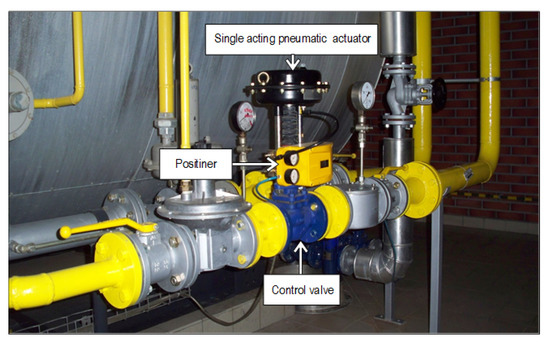
Figure 1.
A snapshot of the exemplary application of an electro-pneumatic final control element in the liquid flow rate control loop in a brewery.
A typical electro-pneumatic final control element consists of three main components: a pneumatic actuator, positioner, and control valve. The stem of the actuator acts on the control valve plug and, thus, throttles the flow of the medium passing through the control valve. The primary goal of the positioner is to control the travel of the stem of the actuator, x, to follow-up the output, , of the external controller, (Figure 2). Clearly, the internal controller, , and the external controller, , constitute a cascade control system, where acts as the secondary controller.
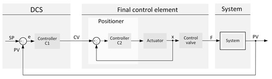
Figure 2.
Conceptual block diagram of a classic, single-loop control system. Notations: —distributed control system; —set point; —process value; e—control error; —primary controller; —digital control signal; —embedded (secondary) controller; x—positioner feedback signal; and, F—flow rate output.
Numerous types of controllers are implemented in positioners. However, a majority of them still apply algorithms. In this paper, we refer exclusively to these types of controllers.
Commonly, the term autotuning is understood as the self-ability of a control device to occasionally, on-demand, or periodically automatically adjust its parameters in order to achieve the required targets of the predefined control quality factors.
Autotuning approaches have been extensively studied, developed, and implemented since the time of Minorsky [1]. Commercially, currently, at least 45 software packages and 39 hardware control modules are available and 80 patents are filed worldwide [2].
Autotuning approaches are the topics of numerous papers, books, studies, and surveys, e.g., [2,3,4,5,6,7,8,9,10,11,12,13,14]. This paper contributes to this area by focusing on the autotuning of specific control systems. Below, we characterize some of the approaches that are considered as milestones in the field of autotuning.
A systematic and easy to implement approaches in regard to controllers were proposed by Ziegler and Nichols [3]. They proposed two variants based on the measurement of the process reaction curve and on the ultimate sensitivity method based on the system settings leading to critical oscillations. They put forward tuning rules for the systems that could be approximated by an effective transfer function as first-order lag systems with a delay. This approximation is applicable to a wide range of industrial systems and, therefore, the Ziegler–Nichols rules are practicable tuning approaches. The Ziegler–Nichols tuning rules attempt to determine the values of three controller settings. However, the obtained settings should not be considered as remarkable promising results of the exact values of the expected overshoot or of an acceptable tracking performance. Both of the above-mentioned control quality factors should be assumed to be crucial for the evaluation of the performances of final control elements.
Åström and Hägglund proposed a simple and transparent off-line autotuning experimental procedure for the adjustment of controller settings [4]. This procedure involved an experiment that allowed for the estimation of the critical gain and the critical frequency of the system. To realize this, they proposed the temporary replacement of the controller with a relay having a known and adjustable amplitude. The resulting oscillations in the system possessed sufficient information regarding the location of the critical point. This allowed for applying the Ziegler–Nichols tuning rules. This simple approach has numerous applications in industrial process control systems. Abundant extensions of this approach have been proposed for tuning model-based and multivariable controllers [7].
A relay autotuner provides a simple approach for identifying parameters; however, the obtained controller settings possess uncertainty that arises from the measurement noise, disturbances, and influence of the choice of the starting point of the tuning procedure. By applying a relay with a hysteresis, the approach becomes less sensitive to the noise. Berner et al. [15] proposed an asymmetric relay autotuner as a remedial solution, to some extent, for the problem of the sensitivity of the adjustment of the controller settings to the noise, disturbances, and starting point of the tuning procedure beyond the non-steady system state.
Industrial autotuners, such as [16], [17], [18], -tuner [18], or from ASEA [19,20], were basically developed for implementation in stand-alone or embedded process controllers, where the computational burden was not problematic. However, this is not so for the two-wire final control elements considered in this study, for which the computational power is extremely limited. adjusts the controller settings adaptively based on pattern recognition of the current process output [2]. The initial parameters are determined by analyzing the process response to small-amplitude artificial excitations. To start an autotuner, the expected noise and the so-called maximum wait-time must be arbitrary preset. This can be considered as an important drawback of this approach. The adaptive feedforward autotuner significantly improves the performance when compared to adaptive feedback control [20].
The -tuner [18] utilizes an asymmetric relay experiment with adjustable amplitudes implemented until the limit cycle is reached. From the oscillations, it derives two parameters that are suitable for obtaining the parameters based on the [5] tuning rules.
In contrast to -tuner, allows for the achievement of shorter experiment times at the expense of larger use of memory and computational power resources [13].
The performance of a relay experiment in regard to its application in the positioner of a final control element is considered to be problematic. The main drawbacks are the following: the unpredictable time of the experiment, sensitivity to the choice of the starting time instant of the experiment, and relatively large demand on the computational power needed, particularly for advanced autotuners. This motivated the search for alternative approaches that could be applicable with some trade-off between the control objectives.
The strong motivation of this work arose directly from the actual demands of a manufacturer of automatic control equipment for the development and implementation of a simple, fast, robust, reliable, and implementable autotuner for the family of single-action electro-pneumatic actuators.
The novelty of the study was the proposition of an original heterogenic autotuner. The heterogeneity of the autotuner resulted from the added-value derived from a combination of three different approaches: identification experiment, expert knowledge, and theoretical findings.
The novel concept was to develop an autotuner that principally mimicked the tuning process performed by an experienced human operator. This finally allowed the adjustment of controller settings based exclusively on a single experimentally identified parameter.
This paper is organized, as follows: the Introductory part briefly reviews the basic autotuning approaches. Thereafter, the motivation, novelty, and contribution of the paper are presented. Section 2 presents and discusses in detail the structure as well as the static and dynamic properties of pneumatic actuators. A set of observations and conclusions drawn from the preliminary experiments is essential for the theoretical background of autotuning presented in Section 3. The autotuning algorithm is described in Section 4. Section 5 presents a discussion of the chosen results of the laboratory experiments, and Section 6 discusses the implementation issues. The concluding remarks, together with the projection of the further research, finalize the paper.
2. Single-Action Pneumatic Actuator
Final control elements are specifically used for the control of gases, liquids, multi-phase agents, and powder flows in control systems. Basically, they can be considered to be electrically controlled mechanical-to-mechanical energy converting devices. In terms of signals, their duty is to convert the control value, , produced by the controller to a mechanical or an electrical physical quantity acting directly on the controlled system.
A single-action pneumatic actuator, positioner, and control valve comprise of a final control element. The positioner is used as a local (auxiliary) controller of the plug displacement of the control valve used for throttling the flow rate of the controlled media.
The simplified diagram of single- and normal-action pneumatic actuator is displayed in Figure 3.
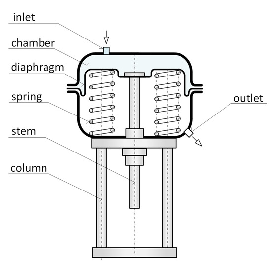
Figure 3.
Simplified cross–sections of single- and normal-action (air-to-close) multi-spring and diaphragm pneumatic actuator.
The travel of the stem of an actuator is due to the imbalance between the static and dynamic forces acting on the diaphragm of the actuator. An active force is developed by the air overpressure acting on the diaphragm. The spring compression force as well as diaphragm elasticity and friction in the bushing oppose the travel of the stem. Additionally, the packing friction, hydrostatic and hydrodynamic forces, as well as d’Alembert forces of the stem, spring, diaphragm, and plug must be considered when an actuator is assembled with a control valve. The detailed phenomenological model of the actuator can be found in [21]. Single-action pneumatic actuators are recognized as devices with a single pressurized chamber. A second chamber remains connected to the surrounding atmosphere. In turn, double-action actuators contain two pressurized chambers. This study deals with single-action actuators exclusively.
Single-action actuators are classified as normal and reverse acting. Alternatively, both the actuators are respectively referred to as air-to-close and air-to-open actuators. The scope of this paper covers the proposition of an autotuner for both types of single-action actuators.
We now discuss the characteristic properties of spring-and-diaphragm actuators. The results of this study will be explained further in this paper. All of the results presented in this section were obtained experimentally.
To make the experiments more reliable, the laboratory set-up (Figure 4) was so arranged that a pneumatic actuator was charged or discharged via an electro-pneumatic transducer used in positioners. This reflected to some extent real working conditions. The instrumentation allowed for measurements of the stem travel, x, of the actuator as well as the air supply pressure, , and the pressure in the chamber of the actuator, p.
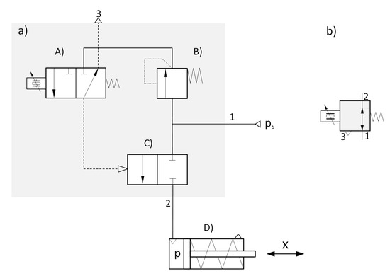
Figure 4.
Block schematics of the experimental set-up for the investigation of the basic features a single-action actuator. (a) electro-pneumatic transducer; (b) schematic symbol. Notations: (A) piezo-pilot valve; (B) pressure regulator; (C) pneumatic booster; and, (D) single action pneumatic actuator.
Step Response
Step response experiments were conducted on a set of 10 different single-action actuators provided by different vendors to obtain more representative data regarding dynamics. Normal as well as reverse-action actuators were investigated. The main construction parameters of the investigated actuators are listed in Table 1. The effective diaphragm areas cover the range [31.2–1000 cm]. The travel is [12.7–50.8 mm] and the volume of the pressure chamber is [0.063–5.00 dcm.

Table 1.
The set of main parameters of the investigated actuators.
All of the actuators were driven by the same electro-pneumatic transducer to maintain the elementary conditions for the comparison of the achieved results.
The step response was obtained by a simple experiment, in which the electro-pneumatic was either switched on when charging or switched off in case of discharging the chamber of the actuator. The step responses of the stem travels were monitored. The following specific features of the investigated actuators were observed:
- a)
- exponential-like shapes of the step response when the chamber was charged,
- b)
- linear-like shapes of the step response when the chamber was discharged,
- c)
- directionality (asymmetry) of the responses, and
- d)
- limited travel of the stem (travel bench range).
Step Responses of the Assembly Pneumatic Actuator and the Electro-Pneumatic Transducer
Let us focus on the exemplary step responses presented in Figure 5.
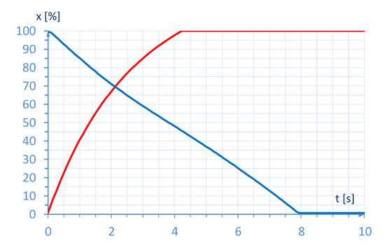
Figure 5.
Illustration of the directionality effect for reverse-action actuator type R1-400 from Polna S.A. The nominal volume of the pressure chamber is 0.800 dcm. The red line depicts retraction and the blue one represents expansion of the stem.
These responses are acquired for single-action actuators with different chamber volumes. The travels of the stems in both the cases are normalized. In the case when the stem is retracted, the step response shifts horizontally left until the origins of both the responses match. For clarity, the effect of the dead zone resulting from the initial compression of the spring is removed from the response.
As can be easily seen from Figure 5 the step responses depend on whether the pressure chamber of the actuator is charged or discharged. This effect will be further referred to as the directionality of the dynamics or briefly as directionality. Directionality manifests a change in the parameters and/or description of the effective transmittance of the actuator.
From the travel step responses that are depicted in Figure 5 the following four important observations regarding control design are made:
- Observation 1. The dynamics of the single-action actuator is strongly dependent on the direction of the stem movement.
- Observation 2. The ratio of the effective time constants in both directions differs significantly.
- Observation 3. The dynamics of the actuator are lower when the chamber is discharged as compared to that when it is charged.
- Observation 4. The empirical categorization of the degree of asymmetry is high [22].
Clearly, the above observations are important when designing a heuristic autotuner. If the chamber of a single-action actuator is charged, then the dynamics of the actuator may be approximated by a first-order lag system. Let us denote and as the effective time constants of the transmittance of the actuator when stem movement of the actuator is either opposed or supported by a spring, respectively. Let the effective dead time in the nominal travel range resulting from the transport delay in the actuator pressure supply pipe and electro-pneumatic transducer dynamics be neglected. The reason is that the dead time of the electro-pneumatic transducer and the air transport time by the short pipe connecting the electro-pneumatic transducer with the chamber of the actuator might be ignored.
The effective time constants as well as their ratio for the ten investigated actuators are listed in Table 2. It must be mentioned that for the studied actuators, the ratio of the effective time constants, , is specific and varies over a wide range from 1.17 to 4.93. This validates Observation 2 and allows the hypothesis that can be expected for single-action actuators.
Table 2.
Parameters of the effective transmittance of the assembly: pneumatic actuator and electro-pneumatic converter.
3. Recovering Unknown Limitations
Clearly, an autotuner has to identify, either directly or indirectly, the parameters of the model of the controlled system. An unexpectedly simple linear dynamic model of a single-action pneumatic actuator is presented in the form of transmittance by a set of formulae (1). The parameters of this model should be experimentally identified prior to setting the appropriate parameters of the stem position controller. The model (1) refers to the normalized values of the pressure and the stem displacement. Therefore, first, both of the values should be measured. However, it can be questioned if this is really necessary. In the following, we will demonstrate that it is sufficient to identify the model parameters by only measuring the stem displacement. This has an important practical effect, because, as a rule, the stem position is measured in each positioner, whereas the pressure in the chamber of an actuator is measured optionally. Moreover, as described earlier, the real travel bench range of the stem is less then the nominal range when assembling a control valve with an actuator. In fact, the real travel range is specific for each pair of assembly actuator–control valve and determined by mechanical limiters as well as montage and machining tolerances. Therefore, it should be defined individually.
Rule 1.
The stem travel range must be measured.
Figure 6 displays the real stem travel range, . The lower and upper bounds of the stem travel are denoted as and , respectively. The theoretical travel range of the stem is . Clearly, the values of and are not directly measurable.
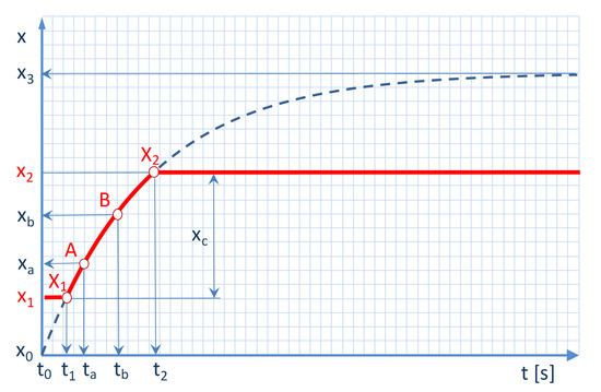
Figure 6.
Illustration of the characteristic points useful for the autotuner.
Let us distinguish between and any additional points and . The question that arises is whether it is possible to restore time constant of the actuator–control valve assembly based on the knowledge of the locations of these points. First, we explain why points and should not be used for this purpose.
Practical note. In practice, there is a portion of uncertainty in determining the time moments when points and are reachable. These time moments can be detected, for example, via robust steady-state detectors. Comparatively, it is more convenient and flexible to acquire the time moments, , corresponding to the characteristic stem position, , inside the stem travel. Notably, this requires making measurements of the stem travel range in advance.
Rule 2.
The characteristic points of the stem step response should be measured using robust approaches.
The stem step response on the supply pressure excitation can be approximated by the formula:
The three unknowns: will be identified based on the knowledge of the coordinates of and .
The simplest method of determining time constant is based on the measurement of time interval between two characteristic points of the response curve. The first point is located in the middle of the theoretical travel of the stem, i.e., , whereas the second point is located at the place where the stem reaches the position, . Hence, and . Finally,
This method seems to be practicable. However, it can still be improved in regard to the robustness, reliability, and usability. When considering the relative pressure bench ranges, either or even both the and points will not be reachable. This does not ensure reliability and usability of the above approach. Moreover, based on the results from (3), the time constant, , is approximately 3.26 times greater than the value of the time interval between time instants and . This may introduce significant uncertainty in the time constant estimation in the case of low-volume actuators, for which the ratio of the resolution of the time measurement to the measured time interval may be as high as 10–20%. Therefore, this approach should be appropriately adopted or reworked to increase its robustness.
Another well-known approach that can be applied to determine the time constant, , is based on the measurement of the time interval, , between two other characteristic points of the step response curve. The first point is located at the beginning of the travel of the theoretical stem, i.e., . The second line is located in the place where the stem reaches position . Hence, and . Finally:
In this case, the time constant is approximately 1.58 times larger than the time interval between time instants, and . This ensures significantly lower uncertainty in the estimation of time constant when compared to that using (3). Nevertheless, the remaining drawbacks of the previous approach are still applicable. Next, we search for the method of estimation of the time constant, , ensuring that points A and B used for its calculation always fall in the true working travel range.
Let us shift the origin of the coordinate system to point A, i.e., by vector . Any point of the exponential curve can be described in both the coordinate systems, as follows:
By introducing appropriate substitutions and transformations, we finally achieve:
Substituting and , we obtain (2). This suggests that shifting the coordinate system in time and space conserves time constant. This feature will be further explored because it reduces the number of unknowns by . This validates Rule 3.
Rule 3.
It is sufficient to examine two different points of the true step response curve to determine the effective time constant and the asymptote of the step response.
Let us now calculate , assuming that the knowledge coordinates correspond to the point, B. (2) results in the following:
From (7), we derive the absolute scale factor, as follows:
Equation (8) is not practical, because it refers to the absolute values of time instants and . A much more practical equation is based on the difference in these times. Substituting and in (6), we obtain
Equation (9) can be interpreted, as follows: the relative stem travel in any time interval is an exponential function of this interval. Equation (9) scales down stem travel with respect to the theoretical travel range, . By making appropriate substitutions, we can also scale down the stem travel, , with respect to the true stem travel.
This validates Rule 4.
Rule 3.
Referencing stem travel in respect to the true travel range ensures that chosen measurement points A and B always belong in the true working range.
Please note that the exponent of the exponential function is invariant to the bias and scaling of its magnitude. Therefore, this feature may be used for fitting the step response into the true step response boundaries, . Shifting the coordinate system in a time range, conserves the time constant too; further, we can freely shift the origin of the response in the time domain. This is depicted in Figure 7, where the origin of the coordinate system is shifted by vector . Clearly, the effective time constant, , is not affected. Therefore, this time constant in the coordinate system, , is the same as that in the original system.
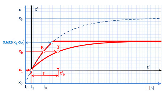
Figure 7.
Illustration of the shift and scale operations.
Let us further scale the step response in a new coordinate system such that it will fit the range, i.e., by the ratio, . Clearly, the scaling operation also does not affect the time constant. Therefore, the time constants of the shifted and scaled responses can be easily obtained by applying, for example, the rule. Let us calculate the ordinates , , and abscissae ( and ), of the points, and B.
(11) states that . This proves Rule 5.
Rule 3.
In practice, measurement of the time instant when the stem starts to move may be imprecise. Therefore, it is recommended to fix time when the stem moves smoothly.
Let us shift the new coordinate system to a new starting point, , such that . In this case, (11) will be rewritten in the form:
This satisfies the requirements of Rule 5 but at the cost of a slight decrease in the travel, , by 5% from 63.2% to 60% of . When , Rule 4 is also satisfied.
Rule 6.
The effective time constant, , when the stem travel of the actuator is opposed by a spring, is lower than the effective time constant, , when the stem of the actuator retracts.
Rule 6 is pure heuristic. However, it is confirmed by a set of experiments performed in order to examine this relation. Please note that the Rule 5 neglects delays in the loop. The delays are strictly depending on the values of technical parameters of both positioner and pneumatic actuator. The significant ratio of time delay to time constant may cause instability of the final control element. Fortunately, in this study, this ratio is below 10% in the worst case. As experiments show relative delay close to 10%, this does not influence the static properties of a positioner. However, in this case, the frequency band should be limited by appropriate setting ramp time constant .
4. Identification Experiment
Identification Algorithm
The discussion that is presented in Section 3 is sufficient to propose an experimental identification algorithm for time constants and . This algorithm seems to be practical because:
- a)
- it is simple and fast,
- b)
- it is irrelevant whether the actuator is working in the normal or reverse mode,
- c)
- the position of the stem of the actuator in the moment of initialization of the identification algorithm is not relevant,
- d)
- its completing time is predictable, and
- e)
- it reduces the uncertainty in the identified parameters by the differential time measurements.
The algorithm consists of seven steps, which are illustrated in Figure 8 and specified in Algorithm 1.
| Algorithm 1: Identification of time constants |
| Algorithm Step 1 - Initialization discharge of the chamber of the actuator Step 2 - Determine limit position a) wait until stem movement is completed b) remember limit position Step 3 - Determine limit position a) charge the chamber of the actuator b) wait until the stem movement is completed c) remember limit position d) calculate stem travel e) normalize stem travel Step 4 - Travel to position a) discharge the chamber of the actuator b) wait until the stem position reaches 95% of the travel bench Step 5 Determine a) start timer b) wait until the stem position reaches 35% of the travel bench c) stop timer d) determine Step 6 - Travel to position a) wait until stem position reaches 5% of the travel bench Step 7 - Determine a) charge the chamber of the actuator b) start timer c) wait until the stem position reaches 65% of the travel bench d) stop timer e) determine |
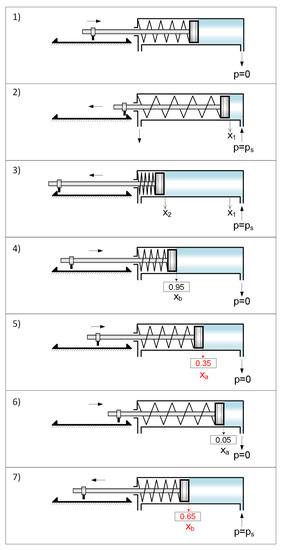
Figure 8.
The sequence of the steps of the experimental part of the autotuner algorithm for single-action electro-pneumatic final control elements.
5. Experiments
The laboratory set-up consists of a mounting rack, a final control element, an air supply station, and a set of instruments. The actuator pressure is regulated either manually via a hand-driven pressure reducing valve or supplied directly from the electro-pneumatic transducer of the positioner. The stem travel is simultaneously measured using the potentiometer of the positioner and an external mechanical dial indicator. The former is mainly employed for dynamic measurements, whereas the latter is for static ones. The air pressure in the chamber of the actuator is measured using a pressure gage. The supplied air pressure is measured by a dial manometer. A PC class computer is used for data acquisition and data processing, as well as for communication with the positioner via a communication interface.
5.1. Methodology
The simplified structure of the investigated final control element is shown in Figure 9.
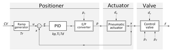
Figure 9.
The structure of the final control element. Notations: —disturbances acting on the pneumatic actuator, —disturbances acting on the control valve, —media pressures on the inlet and outlet of the control valve, F—flow rate of the controlled media. Remaining notations are the same as in previous Figures.
Generally, the experimental efforts were aimed at acquiring some general rules for the selection of the three basic settings: , of an embedded controller as well as of the ramp generator time constant, . The investigations were conducted on arrangements consisting of a specific positioner and different pneumatic actuators and control valves. The ramp time constant, , is defined as the time interval that is required for a 100% change of the positioner setpoint, u, in response to the step of the external control value, . The ramp generator moderates the velocity of the positioner setpoint, u, by factor . The following methodology was adopted for the experiments.
An independent expert with many years of experience in the field of industrial automation systems was invited to tune the controller. The following task has been set to the expert. Four positioner controller parameters (, , , ) shall be experimentally selected for each of the 10 differently sized single-acting pneumatic actuators listed in Table 1, ensuring the shortest possible response time and:
- (a)
- stability in the whole operating range;
- (b)
- robustness of settings changes within ;
- (c)
- aperiodic step response with a maximum overshoot less than ;
- (d)
- the maximum steady-state error not exceeding ; and,
- (e)
- insensitivity on up to % changes in nominal air supply pressure.
No restrictions have been placed before the expert on the duration of the experiments and on the number of tests carried out, provided that, for each type of actuator, the number of these test runs there must be no less than 10. The expert then selected 10 sets of settings from among the tests carried out, which he assessed met the best-formulated control quality criteria. The Figure 10, Figure 11, Figure 12, Figure 13, Figure 14, Figure 15, Figure 16 and Figure 17 show the averaged results of the experiment with the appropriate approximations.
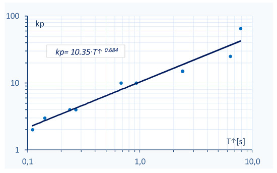
Figure 10.
The proportional gain, , versus the time constant, .
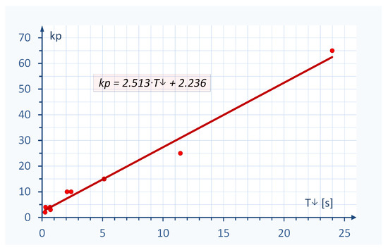
Figure 11.
The proportional gain, , versus the time constant, .
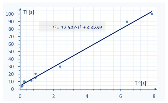
Figure 12.
The integral time, , versus the effective time constant, .
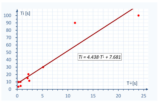
Figure 13.
The integration time, , versus the effective time constant, .
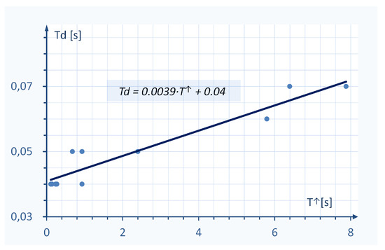
Figure 14.
The derivative time, , versus the time constant, .
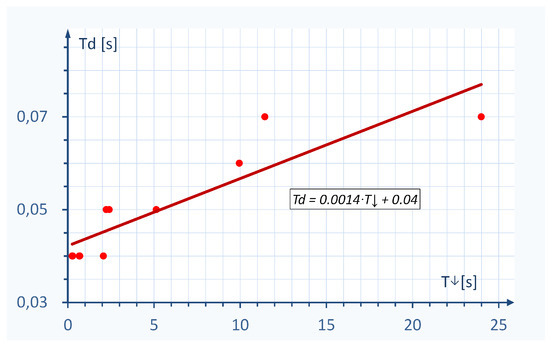
Figure 15.
The derivative time, , versus the time constant, .
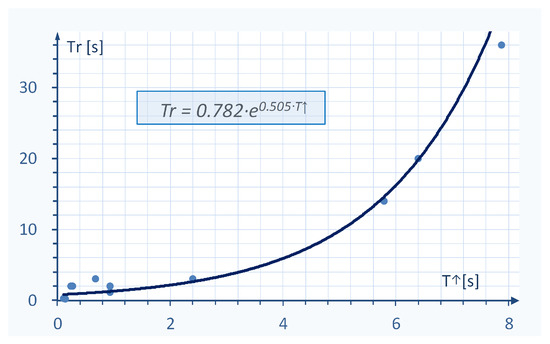
Figure 16.
The ramp time constant, , versus the time constant, .
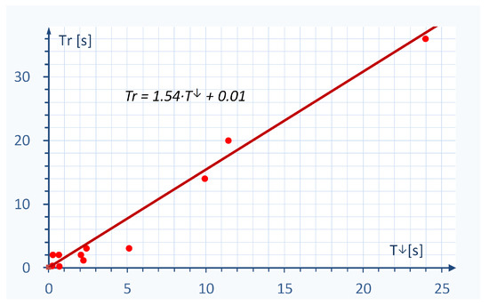
Figure 17.
The ramp time constant, , versus the time constant, .
5.2. Results of the Expert Tuning
The Figure 10, Figure 11, Figure 12, Figure 13, Figure 14, Figure 15, Figure 16 and Figure 17 show the expert settings versus the effective time constants, and . Generally, the obtained results are unexpectedly positively, allowing for formulating extremely simple and implementable heuristic rules for the selection of the positioner controller settings.
Based on Figure 10 and Figure 11 we can formulate the following heuristic rules for expert proportional gain setting:
is proportional to
is proportional to the time constant,
Both the rules suggest that it is sufficient to identify any one of the effective time constants: or , to set the proportional gain of the internal controller analytically from the approximation of or . Remarkably, the coefficients of the linear approximation of the relations: or , are specific for a given positioner. It is supposed that the coefficients of approximation are strongly dependent on the specification of the applied electro-pneumatic transducer and may vary for different positioners. Highly similar rules were derived with respect to the integral time constant, . The results of the experiments that are presented in Figure 12 and Figure 13 can be summarized in the form of two heuristic rules:
is proportional to the time constant,
is proportional to the time constant,
The derivative time constant, , also has quasi-proportional relations with the effective time constants, and , as displayed in Figure 14 and Figure 15. Hence, they follow the rules:
is proportional to the time constant, .
is proportional to the time constant, .
It is clear from Figure 16 that the ramp time constant, , obtained by the expert is an approximate exponential function of the effective time constant, , and it is proportional to the effective time constant, (Figure 17). Hence, it follows the rules:
is an exponential function of the time constant, .
is proportional to the time constant, .
The analysis of the expert tuning results allows at least the formulation of the following general tuning rule.
General rule:
All the settings of a controller intended for application in the positioner of a single-action electro-pneumatic control element can be determined based solely on the effective time constant of the pneumatic actuator either when the chamber of the actuator is being charged or discharged.
This simple rule has very important implications for implementations, because it is promising to obtain all of the controller settings based on only one single experimentally identified parameter. Moreover, the calculations that need to be performed to obtain these settings are notably elementary and do not require to reserve huge memory resources.
It should be mentioned that the above stated rules could also be useful for designing, e.g., a fuzzy-logic-based autotuner [23].
6. Implementation of the Autotuner
To verify the correctness and effectiveness of the proposed heterogenic autotuner, a set of experiments was conducted.
The autotuning algorithm was implemented in an industrial positioner [24] equipped with a 16-bit ultra-low-power micro-controller (MSP430F449) belonging to 430 family from Texas Instruments. This family of micro-controllers is based on memory-to-memory von Neumann architecture, a common address space and reduced orthogonal instruction list. The 430 family is particularly well suited for applications, where the ultra low power consumption is an issue. This is obviously extremely important in case of the two-wire final control devices. The micro-controller of positioner is run by a 4 MHz clock and consumes circa 2.4 mW of power. The sample time of the embedded controller is set to 2.5 ms. The memory resources of microcontroller are quite limited. Together, 60 KB of program flash memory and 2 KB of data RAM memory are allocated to the positioner, including autotuning procedure. The autotuning algorithm is performed in real time. Therefore, the time of the completing this procedure heavily depends on the dynamic properties of the given actuator.
The autotuner software was coded while using a low-level symbolic address programming language. The standard industrial HART communication protocol was used for controlling the experiments and for data acquisition purposes. A few distinct HART functions were added to perform the tests of the autotuner.
All of the ten final control elements with the actuators specified in Table 1 were tested. For each, two tests were performed: static characteristics and step response. Only two control quality criteria were followed: overshoot and steady-state error.
An example of the static characteristics of the final control element with the pneumatic actuator with initial 10% wide hysteresis is shown in Figure 18. The steady-state error drops to tolerance limits. This figure clearly demonstrates the “masking” effect of the internal hysteresis of the assembly: a pneumatic actuator–control valve resulting from the application of the positioner. The hysteresis is close to zero and invisible in the chart. Figure 19 presents the result of the small step response (10%) test performed for normal-action unloaded actuator type Masoneilan 37-13 working under nominal operating conditions. Here, you can see the desired aperiodical step responses throughout the stem travel range. In turn, Figure 20 shows an example of a big step response of the same positioner applied for a reverse-action actuator. In both cases the desired control quality criteria are met.
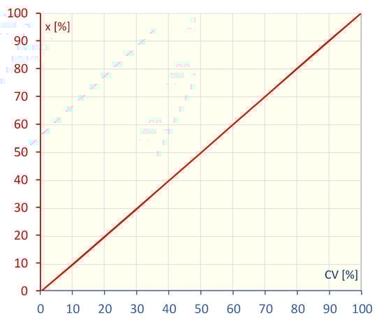
Figure 18.
Illustration of the autotuner quality on example static characteristics of the normal action of a final control element with actuator type Masoneilan 37-09 under nominal operating conditions. Here, the initial hysteresis of the assembly: pneumatic actuator–control valve was 10% wide.
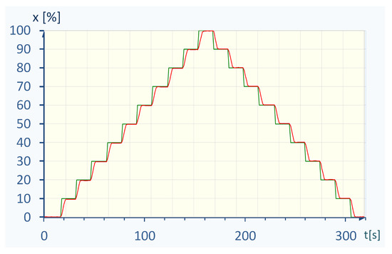
Figure 19.
Illustration of the autotuner quality on the stepwise response of normal-action unloaded actuator type Masoneilan 37-13 under nominal operating conditions. The applied nominal bench range set is [20–100 kPa]. The nominal supply pressure, , is 140 kPa.
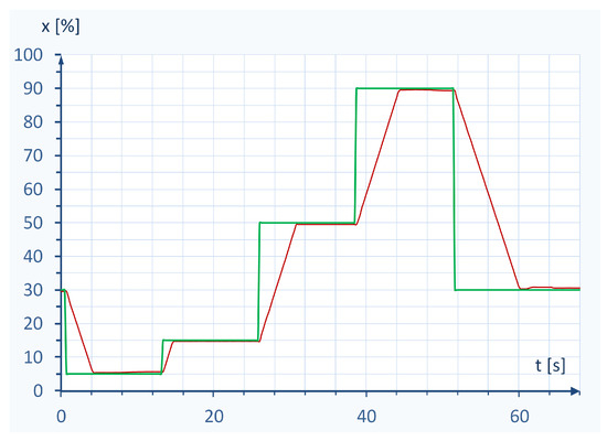
Figure 20.
Illustration of the autotuner quality on the stepwise response of reverse-action actuator type R-400 from Polna S.A. The applied nominal bench range is [80–240 kPa]. The nominal supply pressure, , is 400 kPa. —green line, —red line. Parameters: = 9.6; = 61 s, = 0.07 s; = 15.2 s. Here, we can observe an aperiodic response and close to zero steady-state error.
The autotuning time of the presented approach is dependent on the specification of the electro-pneumatic transducer and the volume of the chamber of the actuator. This time may vary from 20 s for low chamber volumes to 80 s for high chamber volumes. This time should be assumed as acceptable in the context that for some industrial positioners, the autotuning (initialisation) procedure may last even up to dozens of minutes [25]. Figure 21 depicts the experimental autotuning time versus volume of the actuator chamber plot. Here, the autotuning time is almost a linear function of the actuator chamber volume and, therefore, is easy to predict.
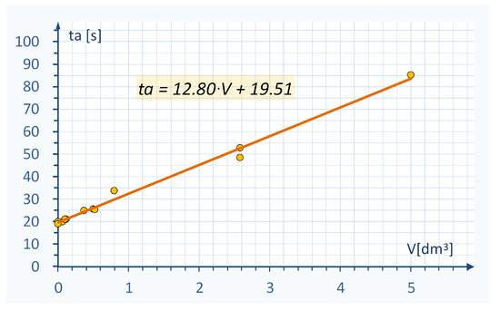
Figure 21.
The overall tuning time versus the volume of the actuator chamber.
7. Summary
In this study, particular attention was paid to the development of a fast, reliable, and robust autotuning algorithm suitable for commissioning, as well as occasional updating of the positioner controller settings.
A novel heterogenic off-line autotuner intended for single-action electro-pneumatic industrial final control elements was proposed. The heterogeneity of the autotuner relied on combining three different approaches: identification experiment, qualitative and quantitative expert knowledge, and theoretical findings. The practical motivation of this work was to propose an easy-to-implement, reliable, and robust autotuner intended for industrial implementations.
First, some heuristic tuning rules of the final control element were found based on the experimental results. As the experiment showed, all of these rules could be referred to the effective time constant of the mechanical assembly of the final control element.
The principles of the identification experiment were validated theoretically. This allows for the implementation of an autotuner that “mimics” the human rules of tuning to some extent. The controller settings were approximated directly from effective time constant–settings curves of the expert.
Similarly, the general rules of the expert tuning were captured experimentally. This allowed the proposition of a general qualitative rule for tuning a controller based on the knowledge of the value of only one time constant. It also permitted relatively fast and reliable automatized commissioning of the final control elements either when setting into production or during periodic maintenance services.
The general rule can be extended for the tuning of the controllers intended for a class of systems exhibiting asymmetric lag and astatic properties that are characterized by a relatively short delays ().
Moreover, the simple implementation with the low requirements of computational and memory resources made this autotuner a mature proposition for manufactures of positioners. The set of performed laboratory and industrial tests demonstrated its usability and performance acceptance.
It was supposed that the simplicity of the tuning rules was partially a derivative of the relatively simple dynamic model of these classes of final control elements. However, a more detailed introspection exhibited static non-linearity, ambiguity, and directional dynamics.
It should be stressed that autotuning algorithm presented in this paper was implemented in industrial positioner and has been verified not only in laboratory but also in numerous industrial applications. The positioner has been produced by one of the Polish companies for more than five years. The autotuner has been successfully validated in many control applications around the world in chemical, petrochemical, power, and food industry.
In the near future, it is planned to develop an effective autotuner that will further reduce the identification experiment turnaround time.
Funding
This research was funded within the Open Science model of the Excellence Initiative Program - Research University of the Warsaw University of Technology.
Conflicts of Interest
The author declares no conflict of interest.
References
- Minorsky, N. Directional stability of automatically steered bodies. J. Am. Soc. Nav. Eng. 1922, 34. [Google Scholar] [CrossRef]
- Ang, K.H.; Chong, G.; Lee, Y. PID Control System Analysis, Design, and Technology. IEEE Trans. Control. Syst. Technol. 2005, 13, 559–576. [Google Scholar]
- Ziegler, J.G.; Nichols, N.B. Optimum settings for automatic controllers. Trans. ASME 1942, 64, 759–768. [Google Scholar] [CrossRef]
- Äström, K.J.; Hägglund, T. Automatic tuning of simple regulators with specifications on phase and amplitude margins. Automatica 1984, 12, 645–651. [Google Scholar] [CrossRef]
- Äström, K.J.; Hägglund, T. PID Controllers: Theory, Design and Tuning; ISA The Instrumentation, Systems, and Automation Society: Research Triangle Park, NC, USA, 1995. [Google Scholar]
- Hang, C.C.; Sin, K.K. A comparative performance study of PID auto–tuners. IEEE Control. Syst. Mag. 1991, 11, 41–47. [Google Scholar]
- Hang, C.C.; Äström, K.J.; Wang, Q.G. Relay feedback auto-tuning of process controllers—A tutorial review. J. Process. Control. 2002, 12, 143–162. [Google Scholar] [CrossRef]
- Wang, T.H. Development of PID Auto-Tuner for TITO Systems. Ph.D. Thesis, Nanyang Technological University, Singapore, 2003. Available online: https://dr.ntu.edu.sg//handle/10356/3684 (accessed on 27 July 2020).
- Yu, C.C. Autotuning of PID Controllers: A Relay Feedback Approach; Springer Science & Business Media: Berlin/Heidelberg, Germany, 2006. [Google Scholar]
- O’Dwyer, A. Handbook of PI and PID Controller Tuning Rules, 2nd ed.; Imperial College Press: London, UK, 2006. [Google Scholar]
- Vilanova, R.; Visioli, A. PID Control in the Third Millennium; Springer: London, UK, 2012. [Google Scholar]
- Alfaro, V.M.; Vilanova, R. Model-Reference Robust Tuning of PID Controllers; Springer: Berlin/Heidelberg, Germany, 2016. [Google Scholar]
- Berner, J.; Soltesz, K.; Hägglund, T.; Äström, K.J. An experimental comparison of PID autotuners. Control. Eng. Pract. 2018, 73, 124–133. [Google Scholar] [CrossRef]
- Chidambaram, M.; Saxena, N. Relay Tuning of PID Controllers: For Unstable MIMO Processes; Springer: Berlin/Heidelberg, Germany, 2018. [Google Scholar]
- Berner, J.; Hägglund, T.; Äström, K.J. Asymmetric relay autotuning—Practical features for industrial use. Control. Eng. Pract. 2016, 54, 21–245. [Google Scholar] [CrossRef]
- Foxboro. Technical Information of EXACT Tuning with 762, 760, and 740 Series Controllers; Technical Report; FOXBORO: Foxboro, MA, USA, 1995. [Google Scholar]
- Honeywell. UDC3200 Universal Digital Controller Product Manual; Honeywell, Doc. Number 51-52-25-119 Revision 5; Honeywell: Charlotte, NC, USA, 2012. [Google Scholar]
- Berner, J.; Soltesz, K. Short and robust experiments in relay autotuners. In Proceedings of the 22nd IEEE International Conference on Emerging Technologies and Factory Automation (ETFA 2017), Limassol, Cyprus, 12–15 September 2017. [Google Scholar]
- Egardt, B. The ASEA Novatune Adaptive Control System. In Proceedings of the NSF-STU Workshop on Adaptive Control, Lund, Sweden, 9–11 July 1984. [Google Scholar]
- Nachtigal, C.L. Adaptive Controller Performance Evaluation: Foxboro EXACT and ASEA Novatune. In Proceedings of the 1986 American Control Conference, Seattle, WA, USA, 18–20 June 1986; pp. 1428–1433. [Google Scholar] [CrossRef]
- Bartyś, M.; Patton, R.; Syfert, M.; de las Heras, S.; Quevedo, J. Introduction to the DAMADICS actuator FDI benchmark study. Control. Eng. Pract. 2006, 14, 577–596. [Google Scholar] [CrossRef]
- Tan, K.; Wang, Q.G.; Lee, T.; Gan, C. Automatic tuning of gain-scheduled control for asymmetrical processes. Control. Eng. Pract. 1998, 6, 1353–1363. [Google Scholar] [CrossRef]
- Lin, Z.; Wei, Q.; Ji, R.; Huang, X.; Yuan, Y.; Zhao, Z. An Electro-Pneumatic Force Tracking System using Fuzzy Logic Based Volume Flow Control. Energies 2019, 12, 4011. [Google Scholar] [CrossRef]
- Aplisens. Electropneumatic Positioner APIS; APLISENS S.A.: Warszawa, Poland, 2018; Available online: https://www.aplisens.com/pdf/produkty/IO.APIS.pdf (accessed on 27 July 2020).
- Siemens. Electropneumatic Positioner for Linear and Part—Turn Actuators; A5E00127926–05; Siemens: Munich, Germany, 2006. [Google Scholar]


© 2020 by the author. Licensee MDPI, Basel, Switzerland. This article is an open access article distributed under the terms and conditions of the Creative Commons Attribution (CC BY) license (http://creativecommons.org/licenses/by/4.0/).