A Methodology for Assembling Future Weather Files Including Heatwaves for Building Thermal Simulations from the European Coordinated Regional Downscaling Experiment (EURO-CORDEX) Climate Data


 ,
,
Abstract
:
1. Introduction
2. State-of-the-Art Future Climate Data Available
2.1. Global Climate Models (GCMs)
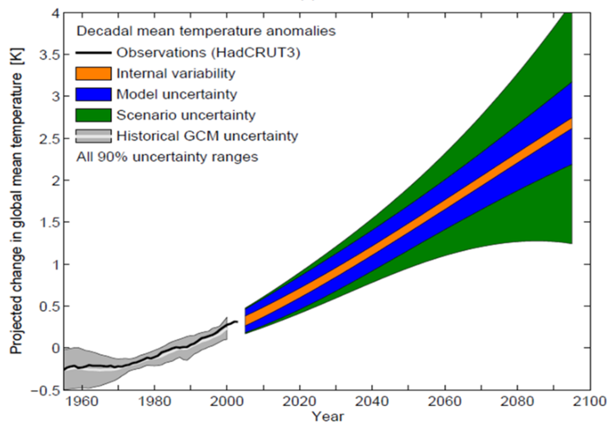
Uncertainties in Global Climate Models
- The uncertainties related to the internal climate variability: these are natural fluctuations of climate from one year to another, or what is commonly called meteorology. For instance, from one year to the next, the weather can be abnormally cold even though the tendency over ten years is a warming temperature.
- The uncertainties related to the climate model that is used from one climate model to another; predictions can vary greatly because the assumptions in the climate models can vary, or some climate aspects may be better represented in one model than another.
- The uncertainties related to the scenario that is considered: this is the uncertainty related to societal development, adaptation, and mitigation policies for climate change.
2.2. Statistical Downscaling
2.2.1. The Morphing Method
2.2.2. Stochastic Weather Generators
2.2.3. Uncertainties in Statistical Downscaling
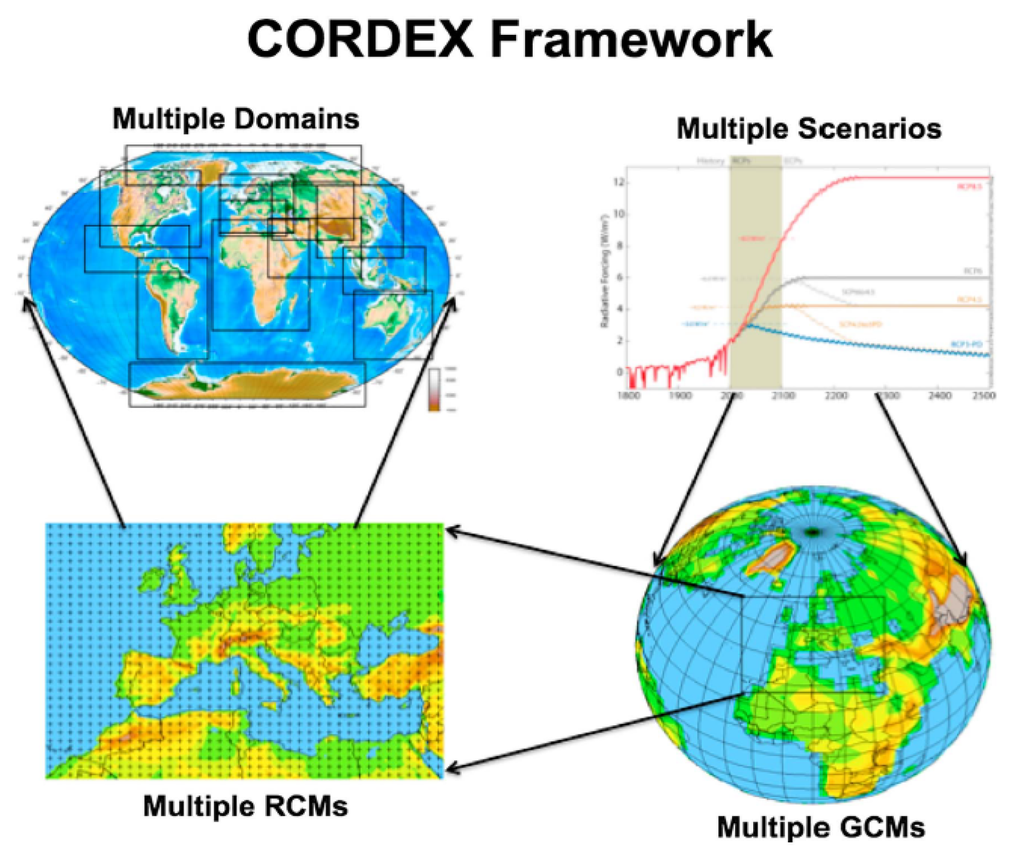
2.3. Dynamical Downscaling (Regional Climate Models)
2.3.1. EURO-CORDEX Climate Data
2.3.2. Uncertainties in Regional Climate Models
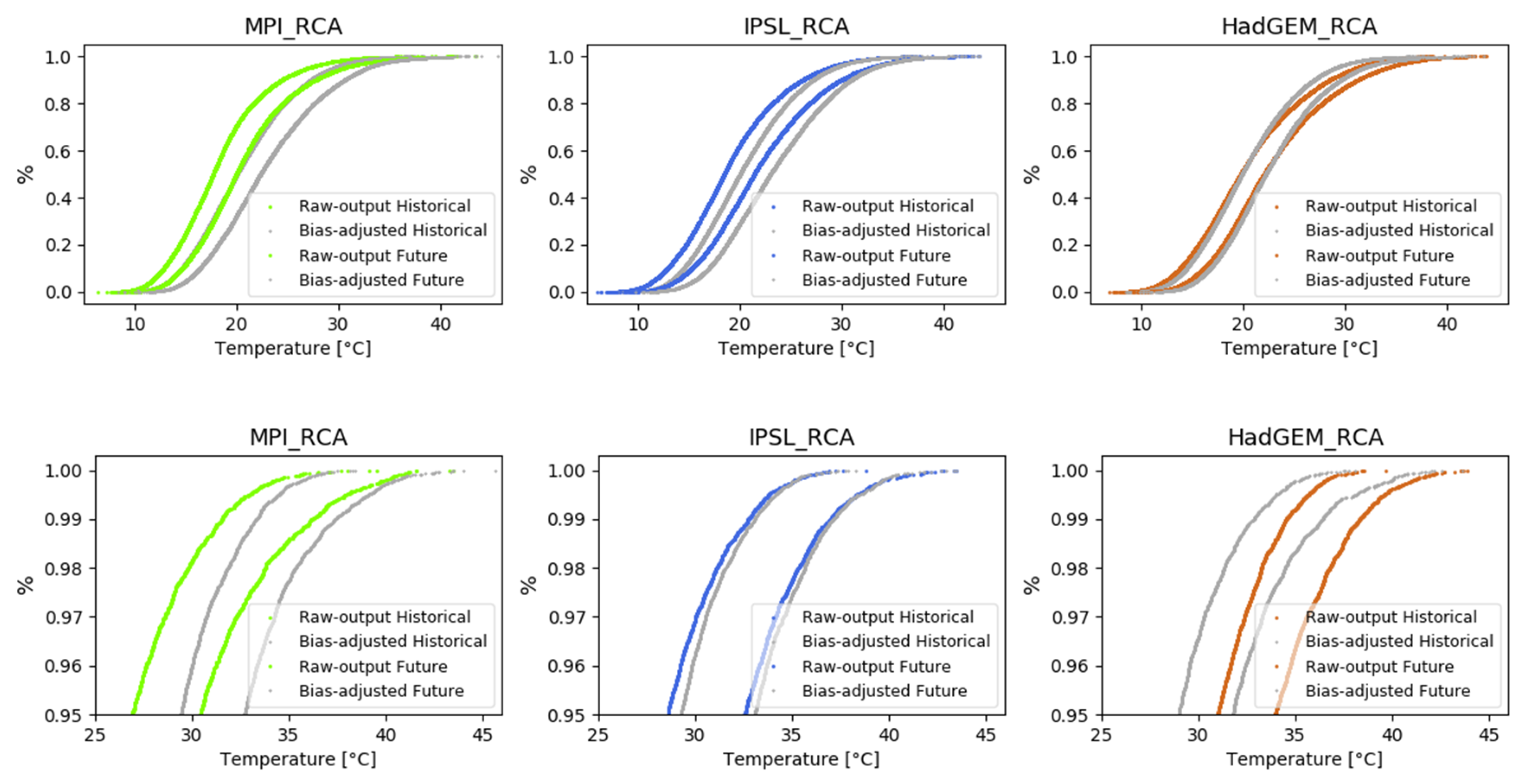
2.3.3. Data Bias in Regional Climate Data
2.4. Comparison of the Downscaling Methods
2.5. Future Weather Files Containing Temperature Extremes
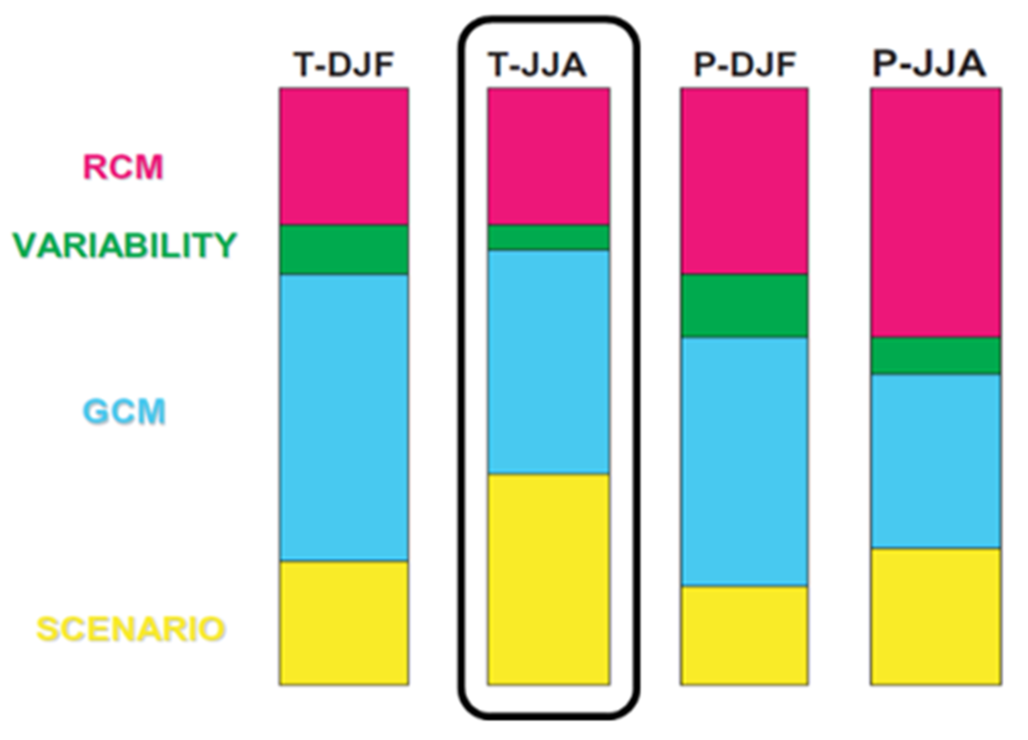
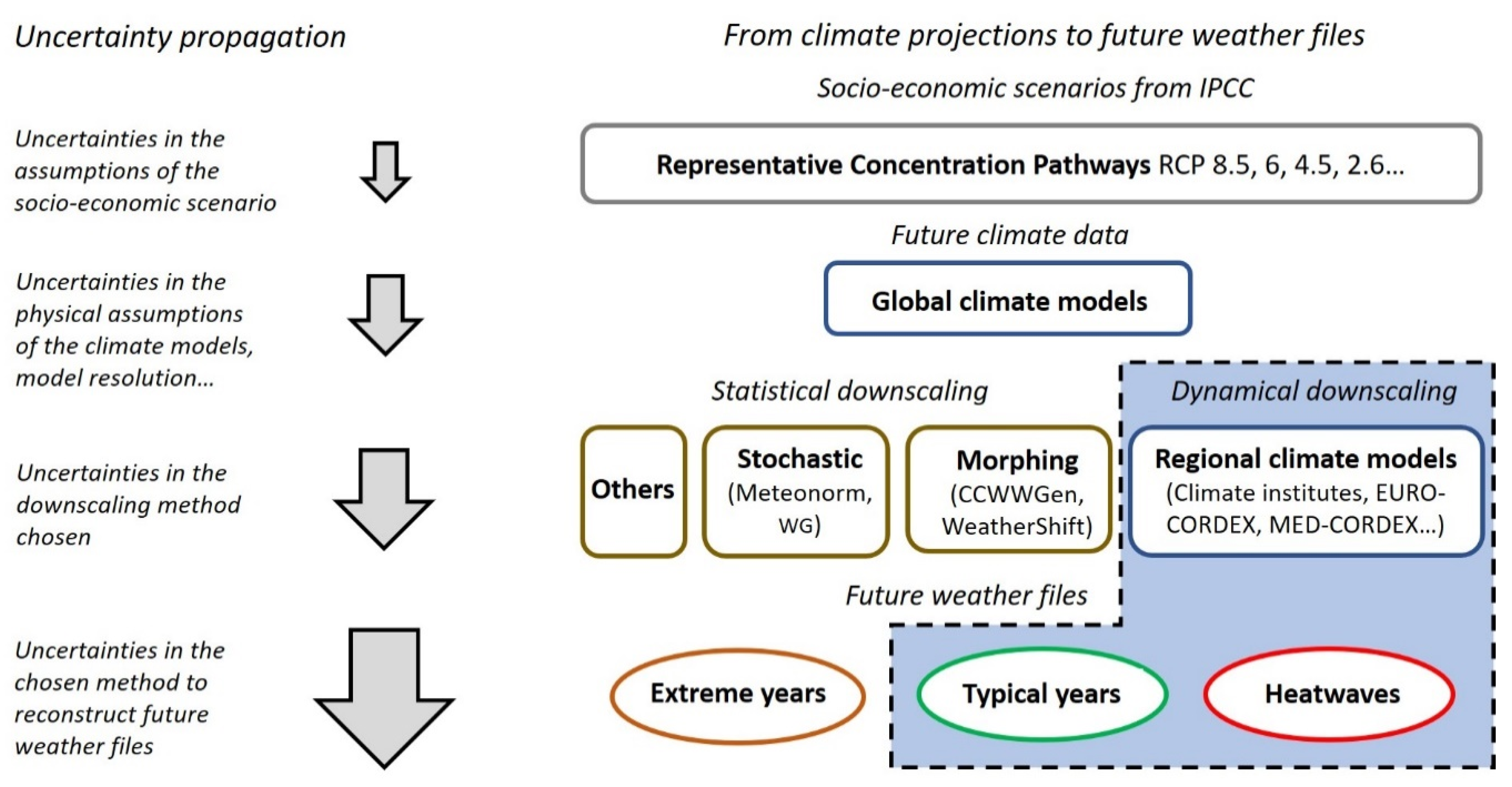
2.6. Uncertainties Propagation from Climate Projections to Future Weather Files
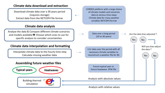
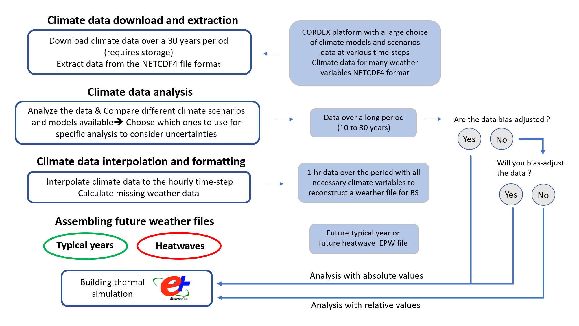
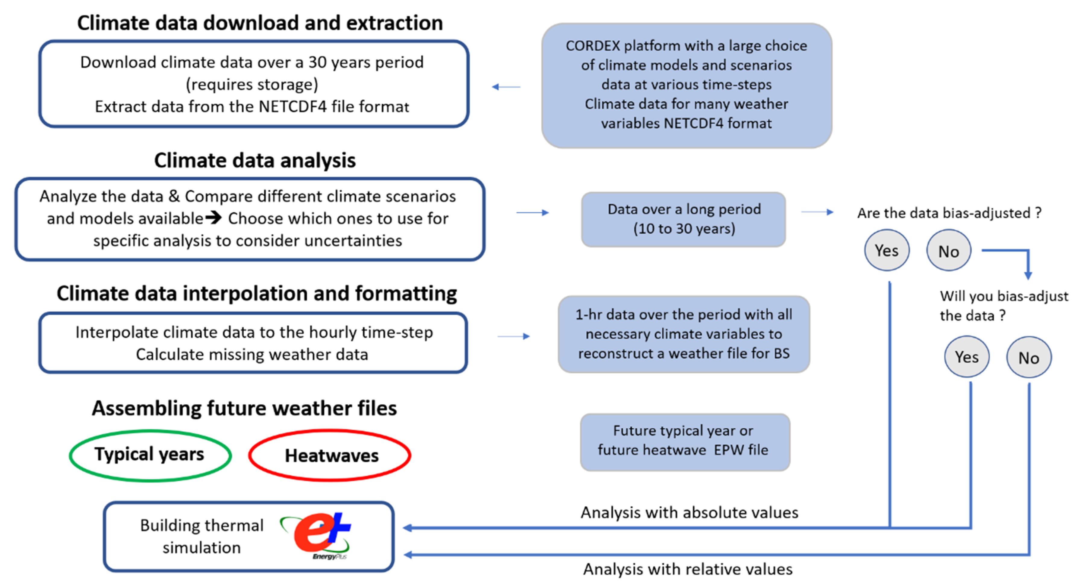
3. Methodology for Assembling Future Weather Files
3.1. Climate Data Download and Extraction from the CORDEX Platform
3.2. Analysis of Climate Data Available on the CORDEX Platform
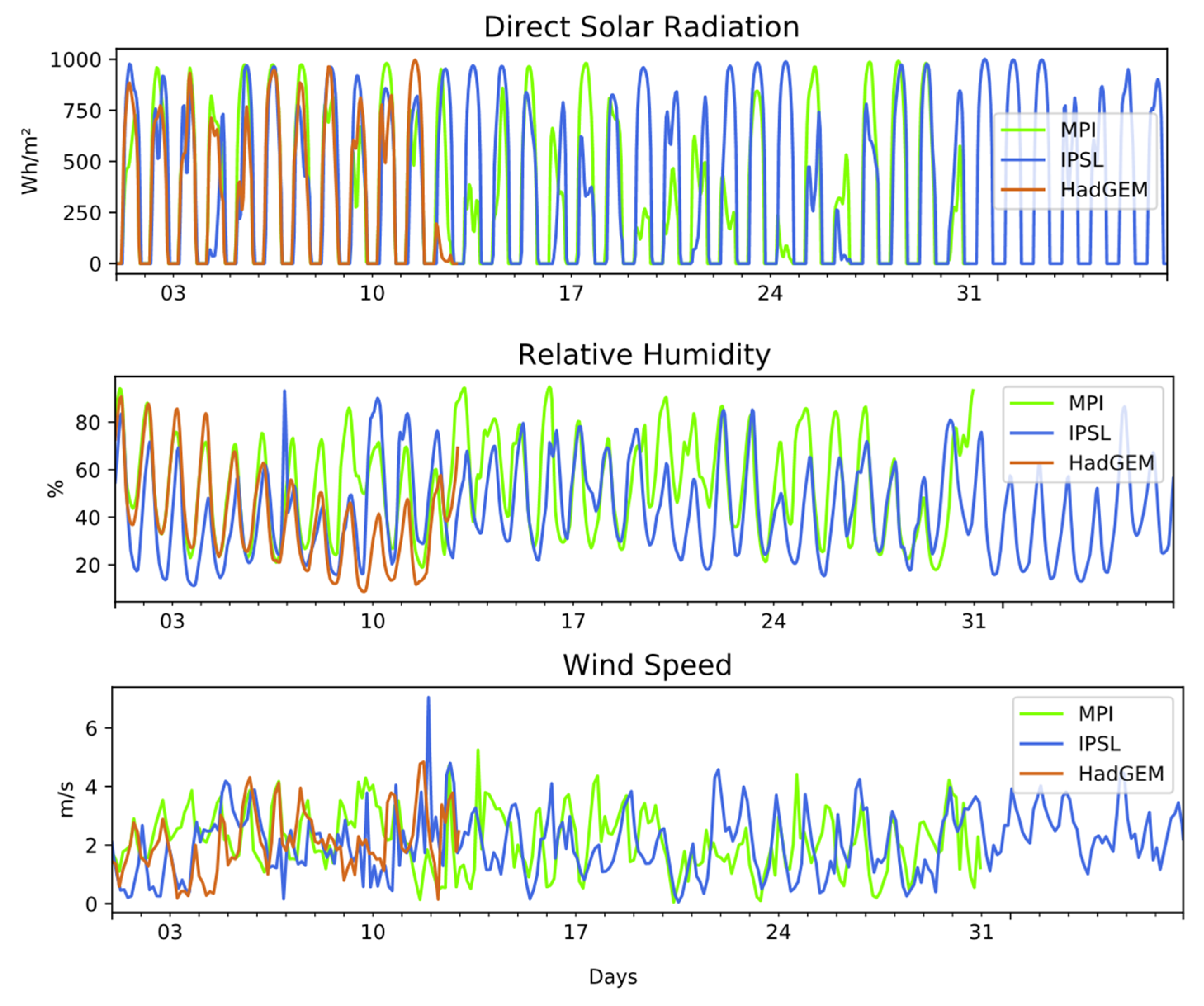
3.3. Data Interpolation and Formatting
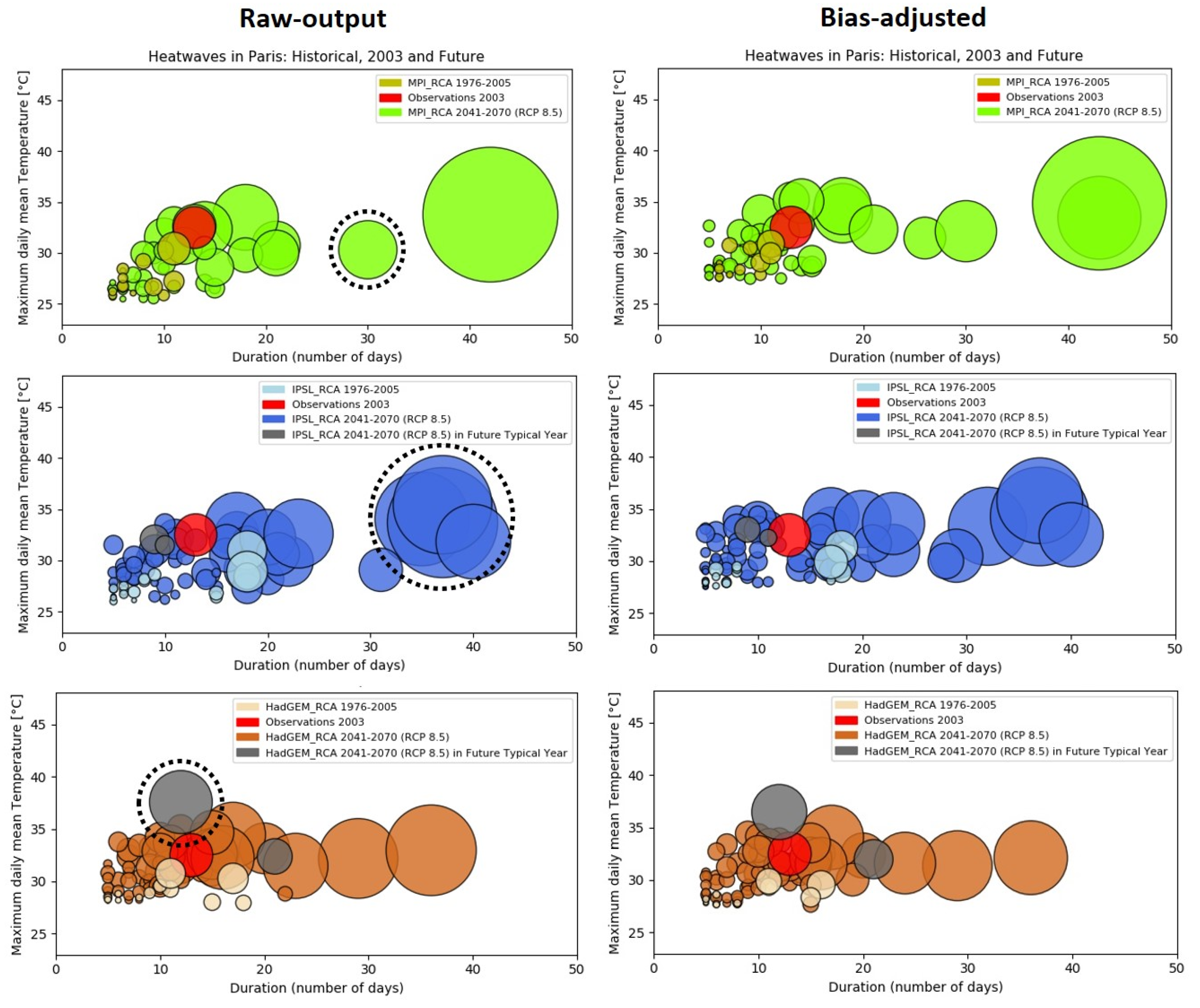
3.4. Assembling Future Weather Files
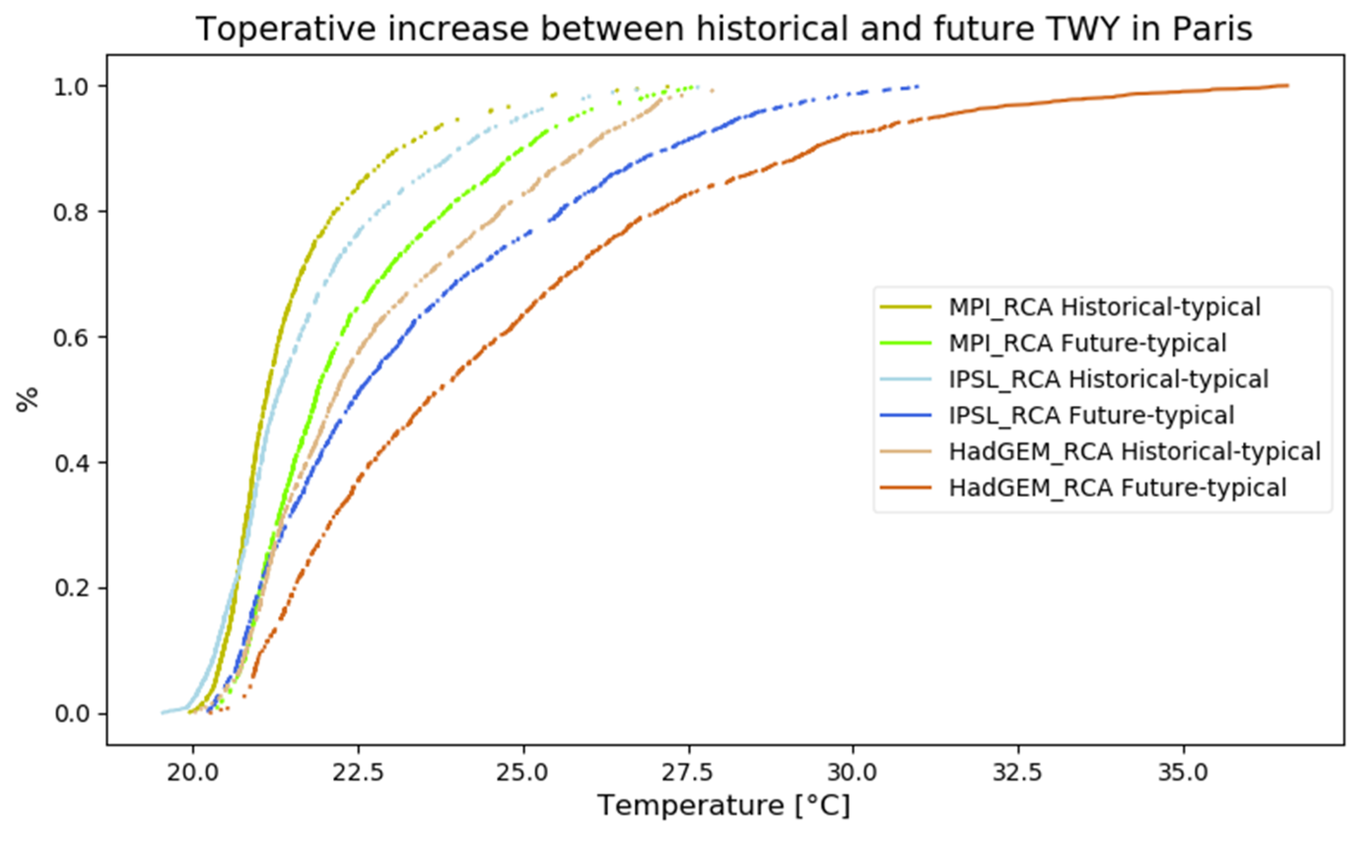
3.4.1. Future Typical Year (TWY)
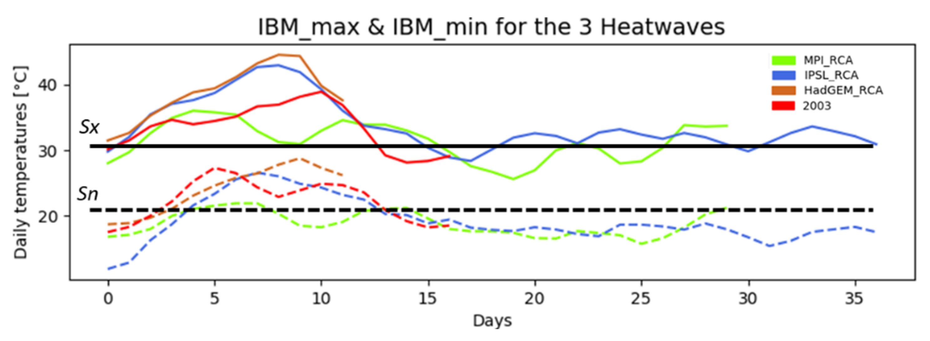
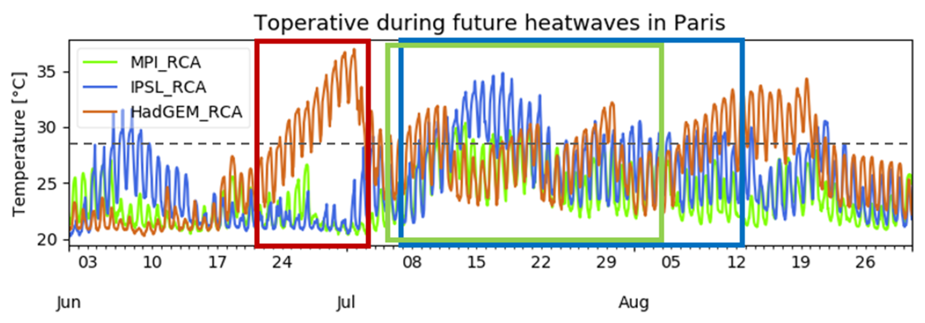
3.4.2. Future Heatwave Event (HWE)
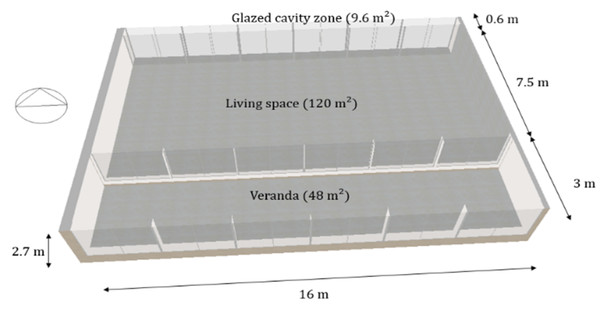
4. Using Future Weather Files for Building Simulations
5. Discussion
6. Conclusions
Author Contributions
Funding
Acknowledgments
Data and Code Availability
Conflicts of Interest
References
- Kjellström, E.; Nikulin, G.; Strandberg, G.; Bøssing Christensen, O.; Jacob, D.; Keuler, K.; Lenderink, G.; Van Meijgaard, E.; Schär, C.; Somot, S.; et al. European climate change at global mean temperature increases of 1.5 and 2 °C above pre-industrial conditions as simulated by the EURO-CORDEX regional climate models. Earth Syst. Dyn. 2018, 9, 459–478. [Google Scholar] [CrossRef] [Green Version]
- Meehl, G.A.; Tebaldi, C. More intense, more frequent, and longer lasting heat waves in the 21st century. Science 2004, 305, 994–997. [Google Scholar] [CrossRef] [PubMed] [Green Version]
- Beniston, M.; Stephenson, D.B.; Christensen, O.B.; Ferro, C.A.T.; Frei, C.; Goyette, S.; Halsnaes, K.; Holt, T.; Jylhä, K.; Koffi, B.; et al. Future extreme events in European climate: An exploration of regional climate model projections. Clim. Chang. 2007, 81, 71–95. [Google Scholar] [CrossRef] [Green Version]
- Fischer, E.M.; Schär, C. Consistent geographical patterns of changes in high-impact European heatwaves. Nat. Geosci. 2010, 3, 398–403. [Google Scholar] [CrossRef]
- Bador, M.; Terray, L.; Boé, J.; Somot, S.; Alias, A.; Gibelin, A.L.; Dubuisson, B. Future summer mega-heatwave and record-breaking temperatures in a warmer France climate. Environ. Res. Lett. 2017, 12, 074025. [Google Scholar] [CrossRef] [Green Version]
- Bessemoulin, P.; Bourdette, N.; Courtier, P.; Manach, J. La canicule d’août 2003 en France et en Europe. La Météorologie 2004, 8, 25. [Google Scholar] [CrossRef] [Green Version]
- Rousseau, D. La Météorologie; Société Météorologique de France: Paris, France, 2005. [Google Scholar] [CrossRef]
- Hémon, D.; Jougla, E. La canicule du mois d’août 2003 en France. Rev. Epidemiol. Sante Publique 2004, 52, 3–5. [Google Scholar] [CrossRef]
- Grignon-Massé, L.; Rivière, P.; Adnot, J. Strategies for reducing the environmental impacts of room air conditioners in Europe. Energy Policy 2011, 39, 2152–2164. [Google Scholar] [CrossRef]
- Santamouris, M. Cooling the buildings—Past, present and future. Energy Build. 2016, 128, 617–638. [Google Scholar] [CrossRef]
- International Energy Agency. The Future of Cooling Opportunities for Energy—Efficient Air Conditioning; International Energy Agency: Paris, Franch, 2018. [Google Scholar]
- Steffen, W.; Hughes, L.; Perkins, S. Heatwaves: Hotter, Longer, More Often; Climate Council of Australia: Potts Point, Australia, 2014; ISBN 9780992414221. [Google Scholar]
- Reeves, J.; Foelz, C.; Grace, P.; Best, P.; Marcussen, T.; Mushtaq, S.; Stone, R.; Loughnan, M.; McEvoy, D.; Ahmed, I.; et al. Impacts and Adaptation Responses of Infrastructure and Communities to Heatwaves: The Southern Australian Experience of 2009; National Climate Change Adaptation Research Facility: Southport, Austrilia, 2010. [Google Scholar]
- Ke, X.; Wu, D.; Rice, J.; Kintner-Meyer, M.; Lu, N. Quantifying impacts of heat waves on power grid operation. Appl. Energy 2016, 183, 504–512. [Google Scholar] [CrossRef]
- Totschnig, G.; Hirner, R.; Müller, A.; Kranzl, L.; Hummel, M.; Nachtnebel, H.P.; Stanzel, P.; Schicker, I.; Formayer, H. Climate change impact and resilience in the electricity sector: The example of Austria and Germany. Energy Policy 2017, 103, 238–248. [Google Scholar] [CrossRef]
- Ribéron, J.; Vandentorren, S.; Bretin, P.; Zeghnoun, A.; Salines, G.; Cochet, C.; Thibault, C.; Hénin, M.; Ledrans, M. Building and Urban Factors in Heat Related Deaths during the 2003 Heat Wave in France. In Proceedings of the Healthy Buildings Conference, Lisboa, Portugal, 4–8 June 2006. [Google Scholar]
- Vandentorren, S.; Bretin, P.; Zeghnoun, A.; Mandereau-Bruno, L.; Croisier, A.; Cochet, C.; Ribéron, J.; Siberan, I.; Declercq, B.; Ledrans, M. August 2003 heat wave in France: Risk factors for death of elderly people living at home. Eur. J. Public Health 2006, 16, 583–591. [Google Scholar] [CrossRef] [PubMed] [Green Version]
- Liu, C.; Kershaw, T.; Fosas, D.; Ramallo Gonzalez, A.P.; Natarajan, S.; Coley, D.A. High resolution mapping of overheating and mortality risk. Build. Environ. 2017, 122, 1–14. [Google Scholar] [CrossRef]
- Taylor, J.; Wilkinson, P.; Picetti, R.; Symonds, P.; Heaviside, C.; Macintyre, H.L.; Davies, M.; Mavrogianni, A.; Hutchinson, E. Comparison of built environment adaptations to heat exposure and mortality during hot weather, West Midlands region, UK. Environ. Int. 2018, 111, 287–294. [Google Scholar] [CrossRef] [Green Version]
- ASHRAE. Chapter 14, Climatic Design Information. In ASHRAE Handbook—Fundamentals 2017; ASHRAE: Peachtree Corners, GA, USA, 2017. [Google Scholar]
- Hacker, J.N.; Belcher, S.E.; Andrew, W. Design Summer Years for London CIBSE TM49: 2014; CIBSE: London, UK, 2014. [Google Scholar]
- Ministère de la Transition Ecologique et Solidaire RE2020: Une Nouvelle Etape vers une Future Règlementation Environnementale des Bâtiments Neufs plus Ambitieuse Contre le Changement Climatique. Available online: https://www.ecologique-solidaire.gouv.fr/re2020-nouvelle-etape-vers-future-reglementation-environnementale-des-batiments-neufs-plus (accessed on 16 April 2020).
- Miller, W.; Machard, A.; Bozonnet, E.; Yoon, N.; Qi, D.; Zhang, C.; Liu, A.; Sengupta, A.; Akander, J.; Hayati, A.; et al. How can we define and measure “resilient cooling”?—A review and evaluation of resilience frameworks and criteria. Submitt. Appl. Energy 2020. submitted for publication. [Google Scholar]
- Folland, C.K.; Karl, T.R.; Christy, J.R.; Clarke, R.A.; Gruza, G.V.; Jouzel, J.; Mann, M.E.; Oerlemans, J.; Salinger, M.J.; Wang, S.-W. 2001: Observed Climate Variability and Change. In Climate Change 2001: The Scientific Basis; Contribution of Working Group I to the Third Assessment Report of the Intergovernmental Panel on Climate Change; Hougton, J.T.Y., Ding, D.J., Griggs, M., Noguer, P., Eds.; Cambridge University Press: Cambridge, UK, 2001; p. 881. [Google Scholar]
- Giorgi, F. Climate change prediction. Clim. Chang. 2005, 73, 239–265. [Google Scholar] [CrossRef]
- Ouzeau, G.; Déqué, M.; Jouini, M.; Planton, S.; Vautard, R.; Jouzel, J. Le Climat de la France au XXIème siècle Volume 4. Scénarios régionalisés: Édition 2014 pour la métropole et les régions d’outre-mer; Rapports de la Direction générale de l’Énergie et du Climat: Paris, France, 2014. [Google Scholar]
- Herrera, M.; Natarajan, S.; Coley, D.A.; Kershaw, T.; Ramallo-González, A.P.; Eames, M.; Fosas, D.; Wood, M. A review of current and future weather data for building simulation. Build. Serv. Eng. Res. Technol. 2017, 38, 602–627. [Google Scholar] [CrossRef] [Green Version]
- Hawkins, E.; Sutton, R. The potential to narrow uncertainty in regional climate predictions. Bull. Am. Meteorol. Soc. 2009, 90, 1095–1108. [Google Scholar] [CrossRef] [Green Version]
- Hawkins, E.; Sutton, R. The potential to narrow uncertainty in projections of regional precipitation change. Clim. Dyn. 2011, 37, 407–418. [Google Scholar] [CrossRef]
- Belcher, S.; Hacker, J.; Powell, D. Constructing design weather data for future climates. Build. Serv. Eng. Res. Technol. 2005, 26, 49–61. [Google Scholar] [CrossRef]
- Jentsch, M.F.; James, P.A.B.; Bourikas, L.; Bahaj, A.B.S. Transforming existing weather data for worldwide locations to enable energy and building performance simulation under future climates. Renew. Energy 2013, 55, 514–524. [Google Scholar] [CrossRef]
- Jentsch, M.F.; Bahaj, A.B.S.; James, P.A.B. Climate change future proofing of buildings-Generation and assessment of building simulation weather files. Energy Build. 2008, 40, 2148–2168. [Google Scholar] [CrossRef]
- Jentsch, M.F. Technical Reference Manual for the CCWeatherGen and CCWorldWeatherGen tools Version 1.2. 2012. Available online: energy.soton.ac.uk/files/2013/06/technical_reference.pdf (accessed on 31 October 2017).
- Troup, L.; Fannon, D. Morphing Climate Data to Simulate Building Energy Consumption. In Proceedings of the ASHRAE and IBPSA-USA SimBuild 2016 Building Performance Modeling Conference, Salt Lake City, UT, USA, 10–12 August 2016; pp. 439–446. [Google Scholar]
- Moazami, A.; Carlucci, S.; Geving, S. Critical Analysis of Software Tools Aimed at Generating Future Weather Files with a view to their use in Building Performance Simulation. Proc. Energy Procedia 2017, 132, 640–645. [Google Scholar] [CrossRef]
- Troup, L.; Eckelman, M.J.; Fannon, D. Simulating future energy consumption in office buildings using an ensemble of morphed climate data. Appl. Energy 2019, 255, 113821. [Google Scholar] [CrossRef]
- Meteonorm. Handbook Part II: Theory, Version 7.2. Global Meteorological Database Version 7, Software and Data for Engineers, Planers and Education. The Meteorological Reference for Solar Energy Applications, Building Design, Heating & Cooling Systems, Education Rene. 2017. Available online: https://meteonorm.com/assets/downloads/mn73_software.pdf (accessed on 1 February 2018).
- Jones, P.; Harpham, C.; Kilsby, C.; Glenis, V.; Burton, A. UK Climate Projections Science Report: Projections of Future Daily Climate for the UK from the Weather Generator. 2010. Available online: https://eprint.ncl.ac.uk/file_store/production/217986/B1B47084-F4B6-446C-A750-8E47554D8B7F.pdf (accessed on 3 November 2019).
- Kershaw, T.; Eames, M.; Coley, D. Assessing the risk of climate change for buildings: A comparison between multi-year and probabilistic reference year simulations. Build. Environ. 2011, 46, 1303–1308. [Google Scholar] [CrossRef] [Green Version]
- Wang, L.; Mathew, P.; Pang, X. Uncertainties in energy consumption introduced by building operations and weather for a medium-size office building. Energy Build. 2012, 53, 152–158. [Google Scholar] [CrossRef] [Green Version]
- Zhai, Z.J.; Helman, J.M. Climate change: Projections and implications to building energy use. Build. Simul. 2019, 12, 585–596. [Google Scholar] [CrossRef]
- Lhotka, O.; Kyseley, J.; Plavcova, E. Evaluation of major heat waves’ mechanisms in EURO-CORDEX RCMs over Central Europe. Clim. Dyn. 2017, 50, 4249–4262. [Google Scholar] [CrossRef]
- Koffi, B.; Koffi, E. Heat waves across Europe by the end of the 21st century: Multiregional climate simulations. Clim. Res. 2008, 36, 153–168. [Google Scholar] [CrossRef] [Green Version]
- Vautard, R.; Gobiet, A.; Jacob, D.; Belda, M.; Colette, A.; Déqué, M.; Fernández, J.; García-Díez, M.; Goergen, K.; Güttler, I.; et al. The simulation of European heat waves from an ensemble of regional climate models within the EURO-CORDEX project. Clim. Dyn. 2013, 41, 2555–2575. [Google Scholar] [CrossRef]
- Giorgi, F. Thirty Years of Regional Climate Modeling: Where Are We and Where Are We Going next? J. Geophys. Res. Atmos. 2019, 124, 5696–5723. [Google Scholar] [CrossRef] [Green Version]
- Jacob, D.; Petersen, J.; Eggert, B.; Alias, A.; Christensen, O.B.; Bouwer, L.M.; Braun, A.; Colette, A.; Déqué, M.; Georgievski, G.; et al. EURO-CORDEX: New high-resolution climate change projections for European impact research. Reg. Environ. Chang. 2014, 14, 563–578. [Google Scholar] [CrossRef]
- Kotlarski, S.; Keuler, K.; Christensen, O.B.; Colette, A.; Déqué, M.; Gobiet, A.; Goergen, K.; Jacob, D.; Lüthi, D.; Van Meijgaard, E.; et al. Regional climate modeling on European scales: A joint standard evaluation of the EURO-CORDEX RCM ensemble. Geosci. Model. Dev. 2014, 7, 1297–1333. [Google Scholar] [CrossRef] [Green Version]
- WRCP Coordinated Downscaling Experiment—European Domain. Available online: https://www.euro-cordex.net/ (accessed on 27 November 2019).
- EUROCORDEX Cordex Archive Specifications. Available online: https://is-enes-data.github.io/cordex_archive_specifications.pdf (accessed on 1 April 2018).
- Moazami, A.; Nik, V.M.; Carlucci, S.; Geving, S. Impacts of future weather data typology on building energy performance—Investigating long-term patterns of climate change and extreme weather conditions. Appl. Energy 2019, 238, 696–720. [Google Scholar] [CrossRef]
- Nik, V.M. Climate Simulation of an Attic Using Future Weather Data Sets—Statistical Methods for Data Processing and Analysis; Chalmers University Of Technology: Göteborg, Sweden, 2010. [Google Scholar]
- Giorgi, F. Regional climate modeling: Status and perspectives. J. Phys. IV EDP Sci. 2006, 139, 101–118. [Google Scholar] [CrossRef]
- Mearns, L.O.; Giorgi, F.; Whetton, P.; Pabon, D.; Hulme, M.; Lal, M. Guidelines for Use of Climate Scenarios Developed from Regional Climate Model Experiments; IPCC: Geneva, Switzerland, 2003. [Google Scholar]
- Lewis, S.C.; King, A.D. Evolution of mean, variance and extremes in 21st century temperatures. Weather Clim. Extrem. 2017, 15, 1–10. [Google Scholar] [CrossRef]
- Russo, S.; Dosio, A.; Graversen, R.G.; Sillmann, J.; Carrao, H.; Dunbar, M.B.; Singleton, A.; Montagna, P.; Barbola, P.; Vogt, J.V. Magnitude of extreme heat waves in present climate and their projection in a warming world. J. Geophys. Res. Atmos. 2014, 119, 12500–12512. [Google Scholar] [CrossRef] [Green Version]
- Alessandrini, J.M.; Ribéron, J.; Da Silva, D. Will naturally ventilated dwellings remain safe during heatwaves? Energy Build. 2019, 183, 408–417. [Google Scholar] [CrossRef] [Green Version]
- Synnefa, A.; Garshasbi, S.; Haddad, S.; Paolini, R.; Santamouris, M. Impact of the mitigation of the local climate on building energy needs in Australian cities. In Proceedings of the Engaging Architectural Science: Meeting the Challenges of Higher Density: 52nd International Conference of the Architectural Science Association 2018, Melbourne, Australia, 28 November–1 December 2018; pp. 277–284. [Google Scholar]
- Pyrgou, A.; Castaldo, V.L.; Pisello, A.L.; Cotana, F.; Santamouris, M. On the effect of summer heatwaves and urban overheating on building thermal-energy performance in central Italy. Sustain. Cities Soc. 2017, 28, 187–200. [Google Scholar] [CrossRef]
- Nik, V.M. Making energy simulation easier for future climate—Synthesizing typical and extreme weather data sets out of regional climate models (RCMs). Appl. Energy 2016, 177, 204–226. [Google Scholar] [CrossRef]
- Ramon, D.; Allacker, K.; van Lipzig, N.P.M.; De Troyer, F.; Wouters, H. Future Weather Data for Dynamic Building Energy Simulations: Overview of Available Data and Presentation of Newly Derived Data for Belgium. In Energy Sustainability in Built and Urban Environments; Springer: Berlin/Heidelberg, Germany, 2018; pp. 111–138. [Google Scholar]
- Liu, C.; Kershaw, T.; Eames, M.E.; Coley, D.A. Future probabilistic hot summer years for overheating risk assessments. Build. Environ. 2016, 105, 56–68. [Google Scholar] [CrossRef]
- Liu, C.; Chung, W.-J.; Coley, D. Creation Of Future Hot Event Years For Assessing Building Resilience Against Future Deadly Heatwaves. In Proceedings of the IBPSA 2019—International Building Performance Simulation Association 2019, Rome, Italy, 2–4 September 2019; Liu, C., Chung, W.-J., Coley, D., Eds.; Centre for Energy and the Design of Environments, University of Bath: Bath, UK, 2019. [Google Scholar]
- Jentsch, M.F.; Eames, M.E.; Levermore, G.J. Generating near-extreme Summer Reference Years for building performance simulation. Build. Serv. Eng. Res. Technol. 2015, 36, 701–721. [Google Scholar] [CrossRef] [Green Version]
- Du, H.; Underwood, C.P.; Edge, J.S. Generating design reference years from the UKCP09 projections and their application to future air-conditioning loads. Build. Serv. Eng. Res. Technol. 2012, 33, 63–79. [Google Scholar] [CrossRef]
- Lemonsu, A.; Beaulant, A.L.; Somot, S.; Masson, V. Evolution of heat wave occurrence over the Paris basin (France) in the 21st century. Clim. Res. 2014, 61, 75–91. [Google Scholar] [CrossRef]
- Lemonsu, A.; Viguié, V.; Daniel, M.; Masson, V. Vulnerability to heat waves: Impact of urban expansion scenarios on urban heat island and heat stress in Paris (France). Urban. Clim. 2015, 14, 586–605. [Google Scholar] [CrossRef]
- Ouzeau, G.; Soubeyroux, J.M.; Schneider, M.; Vautard, R.; Planton, S. Heat waves analysis over France in present and future climate: Application of a new method on the EURO-CORDEX ensemble. Clim. Serv. 2016, 4, 1–12. [Google Scholar] [CrossRef] [Green Version]
- Nik, V.M.; Sasic Kalagasidis, A.; Kjellström, E. Statistical methods for assessing and analysing the building performance in respect to the future climate. Build. Environ. 2012, 53, 107–118. [Google Scholar] [CrossRef]
- ESGF Welcome to the ESGF Node @ IPSL. Available online: https://esgf-node.ipsl.upmc.fr/projects/esgf-ipsl/ (accessed on 27 November 2019).
- EUROCORDEX CORDEX_variables_requirement_table. Available online: https://is-enes-data.github.io/CORDEX_variables_requirement_table.pdf. (accessed on 1 April 2018).
- Kreienkamp, F.; Huebener, H.; Linke, C.; Spekat, A. Good practice for the usage of climate model simulation results—A discussion paper. Environ. Syst. Res. 2012, 1, 9. [Google Scholar] [CrossRef] [Green Version]
- Dufresne, J.L.; Foujols, M.A.; Denvil, S.; Caubel, A.; Marti, O.; Aumont, O.; Balkanski, Y.; Bekki, S.; Bellenger, H.; Benshila, R.; et al. Climate change projections using the IPSL-CM5 Earth System Model: From CMIP3 to CMIP5. Clim. Dyn. 2013, 40, 2123–2165. [Google Scholar] [CrossRef]
- Vrac, M.; Noël, T.; Vautard, R. Bias correction of precipitation through singularity stochastic removal: Because occurrences matter. J. Geophys. Res. 2016, 121, 5237–5258. [Google Scholar] [CrossRef] [Green Version]
- Rasmus, B.; Andreas, H.; Barbara, H.; Tammas, I.; Daniela, J.; Elke, K.-T.; Sven, K.; Grigory, N.; Juliane, O.; Diana, R.; et al. Guidance for EURO-CORDEX Climate Projections Data Use. Available online: https://www.euro-cordex.net/imperia/md/content/csc/cordex/euro-cordex-guidelines-version1.0-2017.08.pdf (accessed on 1 April 2018).
- Terray, L.; Boé, J. Quantifying 21st-century France climate change and related uncertainties. Comptes Rendus Geosci. 2013, 345, 136–149. [Google Scholar] [CrossRef]
- ISO. NF_EN_ISO_15927-2: Performance Hygrothermique des Bâtiments. Calcul et Présentation des Données Climatiques—Partie 2 Donnees Horaires Pour le Dimensionnement de la Charge de Refroidissement; ISO: Geneva, Switzerland, 2009. [Google Scholar]
- ASHRAE. Ashrae Handbook Fundamentals, SI ed.; ASHRAE: Peachtree Corners, GA, USA, 1997. [Google Scholar]
- ISO. ISO NF_EN_ISO_15927-1: Performance Hygrothermique des Bâtiments. Calcul et Présentation des Données Climatiques. Partie 1: Moyennes Mensuelles et Annuelles des Eléments Météorologiques Simples; ISO: Geneva, Switzerland, 2004. [Google Scholar]
- ASHRAE. ASHRAE Fundamentals Handbook; ASHRAE, Ed.; ASHRAE: Peachtree Corners, GA, USA, 2001. [Google Scholar]
- Taesler, R.; Andersson, C. A method for solar radiation computations using routine meteorological observations. Energy Build. 1984, 7, 341–352. [Google Scholar] [CrossRef]
- Young, A.T. Air mass and refraction. Appl. Opt. 1994, 33, 1108–1110. [Google Scholar] [CrossRef] [PubMed]
- ISO. ISO 15927-4: Performance Hygrothermique des Bâtiments. Calcul et Présentation des Données Climatiques. Partie 4: Données Horaires Pour L’évaluation du Besoin Energétique Annuel de Chauffage et de Refroidissement; ISO: Geneva, Switzerland, 2006. [Google Scholar]
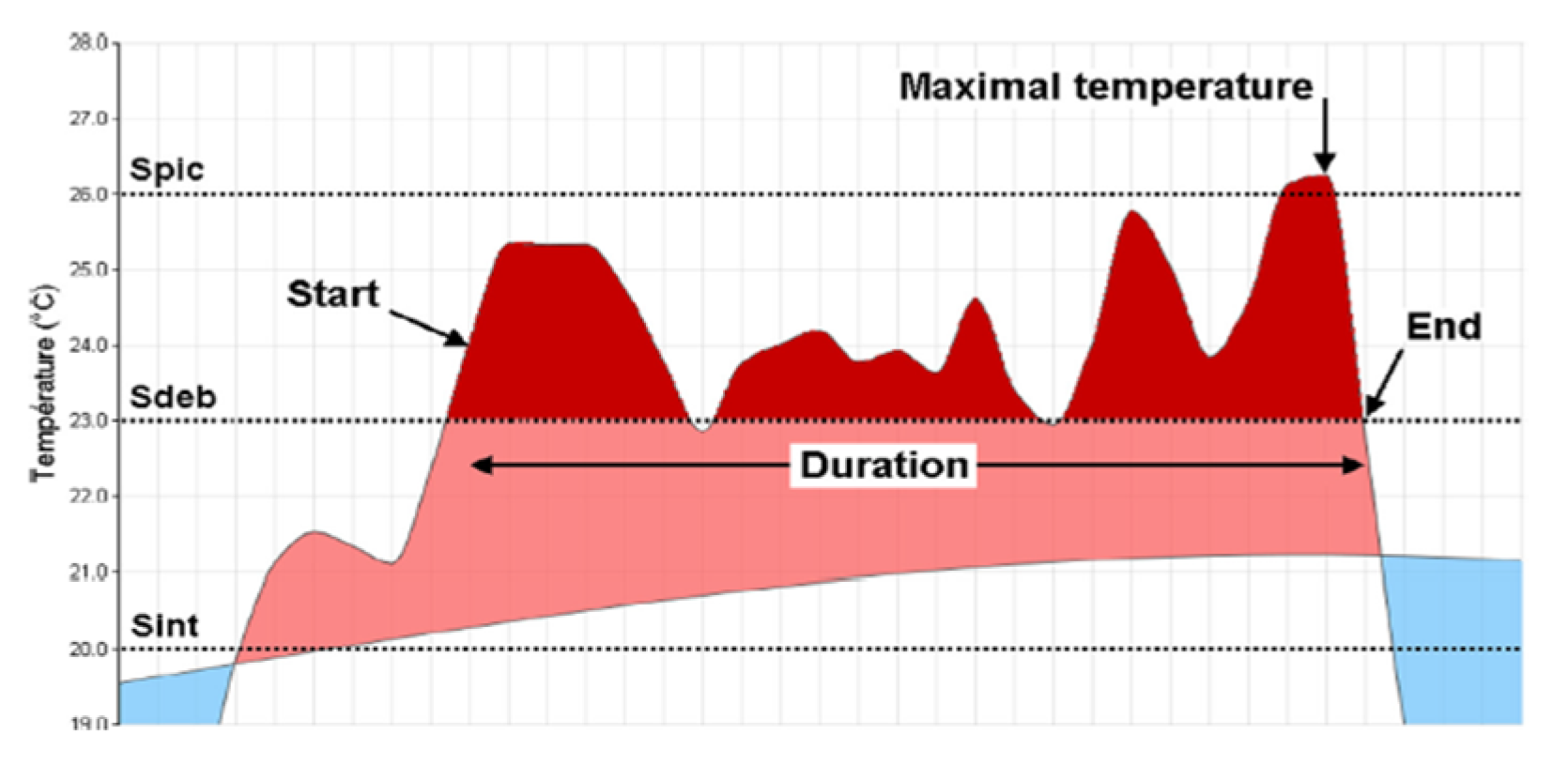
- Robinson, P.J. On the definition of a heat wave. J. Appl. Meteorol. 2001, 40, 762–775. [Google Scholar] [CrossRef]
- Nairn, J.; Fawcett, R. Defining Heatwaves: Heatwave Defined as a Heat-Impact Event Servicing All Communiy and Business Sectors in Australia; Centre for Australian Weather and Climate Research: Melbourne, Australia, 2013. [Google Scholar]
- Nairn, J.R.; Fawcett, R.J.B. The excess heat factor: A metric for heatwave intensity and its use in classifying heatwave severity. Int. J. Environ. Res. Public Health 2014, 12, 227–253. [Google Scholar] [CrossRef] [PubMed] [Green Version]
- Perkins, S.E.; Alexander, L.V. On the measurement of heat waves. J. Clim. 2013, 26, 4500–4517. [Google Scholar] [CrossRef]
- Soubeyroux, J.-M.; Ouzeau, G.; Schneider, M.; Cabanes, O.; Kounkou-Arnaud, R. Les vagues de chaleur en France: Analyse de l’été 2015 et évolutions attendues en climat futur. La Météorologie 2016, 8, 45. [Google Scholar] [CrossRef] [Green Version]
- Laaidi, K.; Ung, A.; Wagner, V.; Beaudeau, P.; Pascal, M. The French Heat and Health Watch Warning System: Principles, fundamentals and assessment; Institut de Veille Sanitaire: Saint-Maurice, Franch, 2013; Volume 20. [Google Scholar]
- RTE. Bilan Prévisionnel de L’équilibre Offre-Demande D’électricité en FRANCE; RTE: Donnybrook, Ireland, 2017. [Google Scholar]
- Cox, R.A.; Drews, M.; Rode, C.; Nielsen, S.B. Simple future weather files for estimating heating and cooling demand. Build. Environ. 2015, 83, 104–114. [Google Scholar] [CrossRef] [Green Version]
- Arima, Y.; Ooka, R.; Kikumoto, H.; Yamanaka, T. Effect of climate change on building cooling loads in Tokyo in the summers of the 2030s using dynamically downscaled GCM data. Energy Build. 2016, 114, 123–129. [Google Scholar] [CrossRef]
- Bravo Dias, J.; Carrilho da Graça, G.; Soares, P.M.M. Comparison of methodologies for generation of future weather data for building thermal energy simulation. Energy Build. 2020, 206, 109556. [Google Scholar] [CrossRef]
- Van Hooff, T.; Blocken, B.; Hensen, J.L.M.; Timmermans, H.J.P. Reprint of: On the predicted effectiveness of climate adaptation measures for residential buildings. Build. Environ. 2015, 83, 142–158. [Google Scholar] [CrossRef] [Green Version]
- Royé, D. The effects of hot nights on mortality in Barcelona, Spain. Int. J. Biometeorol. 2017, 61, 2127–2140. [Google Scholar] [CrossRef] [PubMed]
- Guo, S.; Yan, D.; Hong, T.; Xiao, C.; Cui, Y. A novel approach for selecting typical hot-year (THY) weather data. Appl. Energy 2019, 242, 1634–1648. [Google Scholar] [CrossRef] [Green Version]
- Coley, D.; Kershaw, T.; Eames, M. A comparison of structural and behavioural adaptations to future proofing buildings against higher temperatures. Build. Environ. 2012, 55, 159–166. [Google Scholar] [CrossRef] [Green Version]
- Masson, V.; Marchadier, C.; Adolphe, L.; Aguejdad, R.; Avner, P.; Bonhomme, M.; Bretagne, G.; Briottet, X.; Bueno, B.; de Munck, C.; et al. Adapting cities to climate change: A systemic modelling approach. Urban. Clim. 2014, 10, 407–429. [Google Scholar] [CrossRef]
- Machard, A.; Inard, C.; Alessandrini, J.-M.; Pelé, C.; Ribéron, J. Should we design buildings for future typical summers or future heatwaves? In Proceedings of the Windsor Conference, Windsor Great Park, UK, 16–19 April 2020. [Google Scholar]
- Lapisa, R.; Bozonnet, E.; Salagnac, P.; Abadie, M.O. Optimized design of low-rise commercial buildings under various climates—Energy performance and passive cooling strategies. Build. Environ. 2018, 132, 83–95. [Google Scholar] [CrossRef]
- Moazami, A.; Carlucci, S.; Nik, V.M.; Geving, S. Towards climate robust buildings: An innovative method for designing buildings with robust energy performance under climate change. Energy Build. 2019, 202, 109378. [Google Scholar] [CrossRef]
- Campisi, D.; Gitto, S.; Morea, D. An evaluation of energy and economic efficiency in residential buildings sector: A multi-criteria analisys on an Italian case study. Int. J. Energy Econ. Policy 2018, 8, 185–196. [Google Scholar]
- Ren, Z.; Chen, Z.; Wang, X. Climate change adaptation pathways for Australian residential buildings. Build. Environ. 2011, 46, 2398–2412. [Google Scholar] [CrossRef]
- Perera, A.T.D.; Nik, V.M.; Chen, D.; Scartezzini, J.L.; Hong, T. Quantifying the impacts of climate change and extreme climate events on energy systems. Nat. Energy 2020, 5, 150–159. [Google Scholar] [CrossRef] [Green Version]


| Statistical (Morphing, Stochastic) | Dynamical (Regional Climate Models) | |
|---|---|---|
| Advantages | Simple method Low computational power Energy Plus Weather (EPW) files (future typical years) ready to use for building simulations | Physically consistent datasets across different weather variables Extreme events (such as heatwaves) are well represented |
| Disadvantages | Climate change is only represented through monthly averages Lack of physical consistency between weather variables Future extreme events are not represented Models and scenarios used depend on the tool, which makes it difficult to assess uncertainties Analogies to present-day climate, assumptions that future weather patterns will be similar to present-day observations | High storage capacity needed All data needed to reconstruct a weather file not available at the hourly format yet on the CORDEX platform (3 h time-step data available) Formatting and interpolations are required to reconstruct an EPW file (time-consuming and requires some knowledge) Most data on the CORDEX platform are not bias-adjusted |
| Institution | Driving GCM | CMIP5 Ensemble Member | RCM_VersionID | Date Uploaded on the CORDEX Platform | GCM_RCM Combination Short-Name |
|---|---|---|---|---|---|
| SMHI (1) | CNRM-CERFACS-CNRM-CM5 | r1i1p1 | RCA4_v1 | 2018-02-26 | CNRM_RCA |
| CNRM (2) | CNRM-CERFACS-CNRM-CM5 | r1i1p1 | ALADIN63_v2 | 2019-04-19 | CNRM_ALADIN |
| SMHI | NorESM1-M | r1i1p1 | RCA4_v1 | 2018-08-20 | NorESM_RCA |
| SMHI | MPI-M-MPI-ESM-LR (5) | r1i1p1 | RCA4_v1 | 2018-02-26 | MPI_RCA |
| GERICS (3) | MPI-M-MPI-ESM-LR | r3i1p1 | REMO2015_v1 | 2019-09-25 | MPI_REMO |
| ITCP (4) | MPI-M-MPI-ESM-LR | r1i1p1 | RegCM4-6_v1 | 2019-05-02 | MPI_RegCM |
| SMHI | ICHEC-EC-EARTH | r12i1p1 | RCA4_v1 | 2018-02-26 | EC-EARTH_RCA |
| SMHI | IPSL-IPSL-CM5A-MR | r1i1p1 | RCA4_v1 | 2018-02-26 | IPSL_RCA |
| SMHI | MOHC-HadGEM2-ES | r1i1p1 | RCA4_v1 | 2018-02-26 | HadGEM_RCA |
| SMHI | MOHC-HadGEM2-ES | r1i1p1 | ALADIN63_v1 | 2019-10-04 | HadGEM_ALADIN |
| SMHI | MOHC-HadGEM2-ES | r1i1p1 | RegCM4-6_v1 | 2019-05-02 | HadGEM_RegCM |
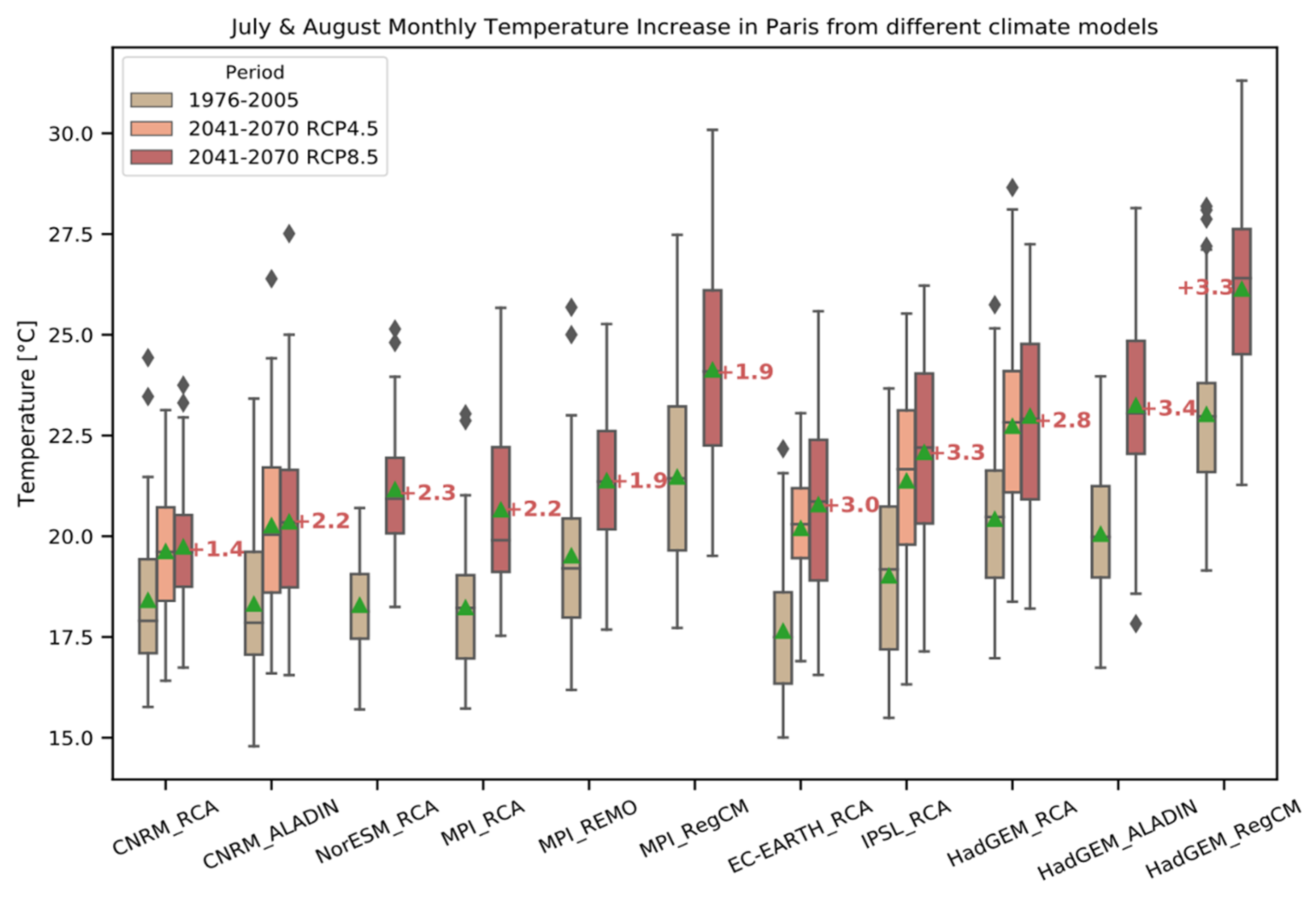
| Centile | MPI_RCA | IPSL_RCA | HadGEM_RCA | Uncertainty of Temperature Increase |
|---|---|---|---|---|
| 0.5 centile (7440 h) | +2.3 °C | +3.0 °C | +2.3 °C | 23% |
| 0.95 centile (744 h) | +3.5 °C | +4.1 °C | +2.9 °C | 29% |
| 0.99 centile (149 h) | +4.7 °C | +4.5 °C | +3.8 °C | 15% |
| Climate Variable from EURO-CORDEX Every 3 h | Data Point Type | Interpolation Method to the Hourly Time-Step | Climate Variable Needed for the EPW File (Department of Energy, 2017) | Equations Used to Calculate the Missing Climate Variable |
|---|---|---|---|---|
| Dry-bulb temperature (K) | Data point * | Polynomial order (n − 1) with n the number of points per day | Dry-bulb Temperature (°C) | - |
| Specific Humidity (kg/kg) | Data point * | Linear | Relative Humidity (%), Dew-Point Temperature (°C) | Equations (1)–(3) |
| Atmospheric Pressure | Data point * | Linear | Atmospheric Pressure (Pa) | - |
| Cloud cover (%) | Average ** | Linear | Direct Normal Radiation Horizontal Infrared Radiation Intensity (Wh/m2) | Equations (4)–(14) and (17)–(18) |
| Global Horizontal Radiation (W/m2) | Average ** | Polynomial order (n − 1) with n the number of points per day | Diffuse Horizontal Radiation (Wh/m2) | Equations (15)–(16) |
| Wind Speed (m/s) | Data point * | Linear | Wind Speed (m/s) | - |
| No climate variable | No data | - | Wind Direction (deg) | - |
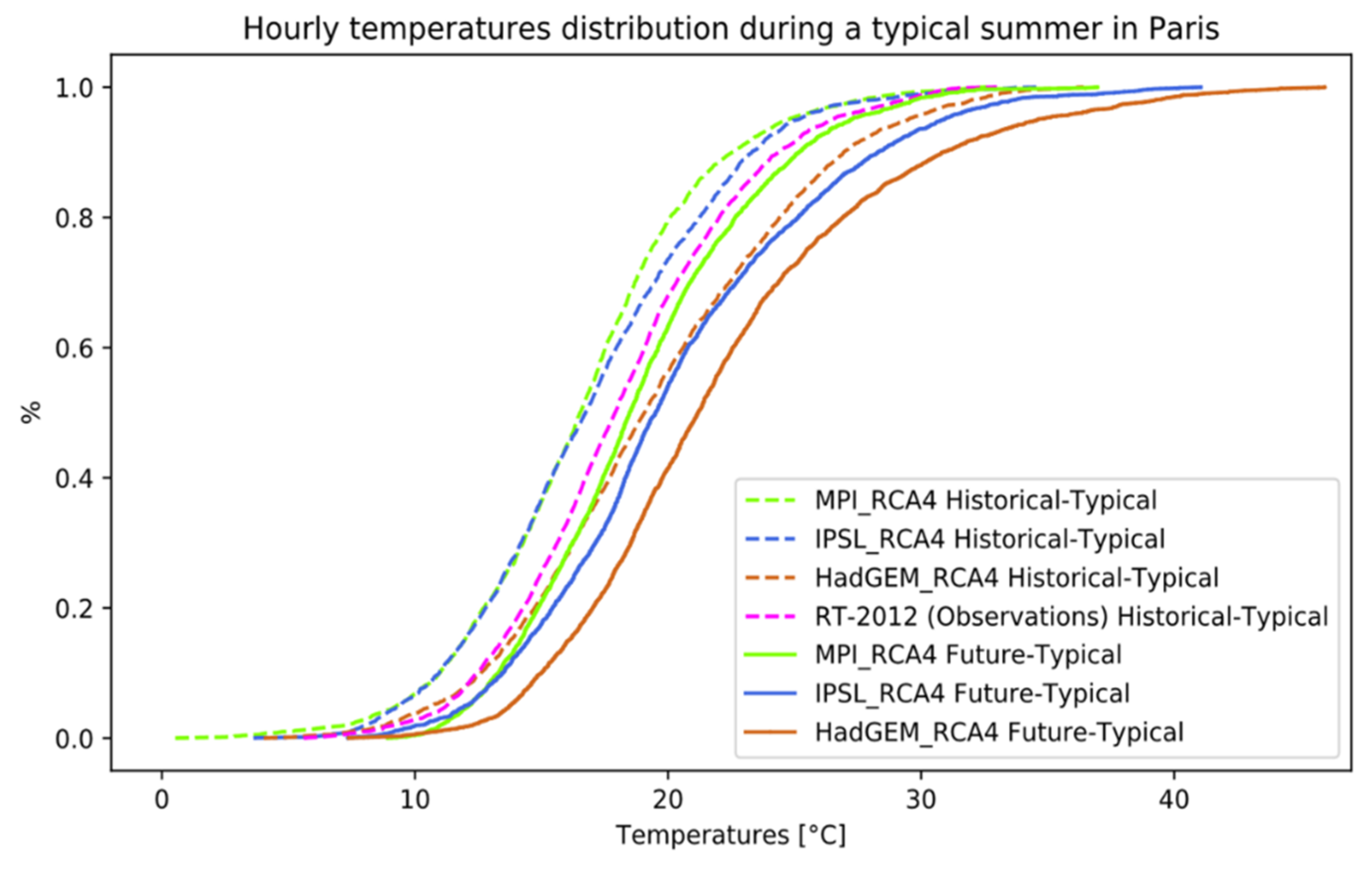
| Series of Daily Averages of the Climate Variable Classified in Ascending Order (Year 2041 to 2070) | Series of Daily Averages of the Climate Variable Classified in Ascending Order (y = 2041) | |||
|---|---|---|---|---|
| 1 | 0.0010 | −7.75 | 0.03 | −0.99 |
| 2 | 0.0021 | −7.53 | 0.06 | −0.48 |
| 3 | 0.0032 | −7.52 | 0.09 | −0.01 |
| Location | Data Type | Climate Model(s) | Sint (95) | Sdeb (97.5) | Spic (99.5) |
|---|---|---|---|---|---|
| Paris | Raw-output | MPI_RCA | 20.76 | 22.27 | 25.40 |
| Paris | Raw-output | IPSL_RCA | 21.19 | 22.97 | 25.88 |
| Paris | Raw-output | HadGEM_RCA | 23.44 | 25.22 | 27.85 |
| Paris | Raw-output | Median of the 3 models | 21.19 (2.68) | 22.97 (2.95) | 25.88 (2.45) |
| Paris | Bias-adjusted | Median of the 3 models | 22.9 (0.15) | 24.39 (0.14) | 27.48 (0.38) |
| France [67] | Bias-adjusted | Median of 11 models | 20.67 (0.10) | 22.03 (0.16) | 24.27 (0.20) |
© 2020 by the authors. Licensee MDPI, Basel, Switzerland. This article is an open access article distributed under the terms and conditions of the Creative Commons Attribution (CC BY) license (http://creativecommons.org/licenses/by/4.0/).
Share and Cite
Machard, A.; Inard, C.; Alessandrini, J.-M.; Pelé, C.; Ribéron, J. A Methodology for Assembling Future Weather Files Including Heatwaves for Building Thermal Simulations from the European Coordinated Regional Downscaling Experiment (EURO-CORDEX) Climate Data. Energies 2020, 13, 3424. https://doi.org/10.3390/en13133424
Machard A, Inard C, Alessandrini J-M, Pelé C, Ribéron J. A Methodology for Assembling Future Weather Files Including Heatwaves for Building Thermal Simulations from the European Coordinated Regional Downscaling Experiment (EURO-CORDEX) Climate Data. Energies. 2020; 13(13):3424. https://doi.org/10.3390/en13133424
Chicago/Turabian StyleMachard, Anaïs, Christian Inard, Jean-Marie Alessandrini, Charles Pelé, and Jacques Ribéron. 2020. "A Methodology for Assembling Future Weather Files Including Heatwaves for Building Thermal Simulations from the European Coordinated Regional Downscaling Experiment (EURO-CORDEX) Climate Data" Energies 13, no. 13: 3424. https://doi.org/10.3390/en13133424
APA StyleMachard, A., Inard, C., Alessandrini, J.-M., Pelé, C., & Ribéron, J. (2020). A Methodology for Assembling Future Weather Files Including Heatwaves for Building Thermal Simulations from the European Coordinated Regional Downscaling Experiment (EURO-CORDEX) Climate Data. Energies, 13(13), 3424. https://doi.org/10.3390/en13133424