Real-Time Building Smart Charging System Based on PV Forecast and Li-Ion Battery Degradation

Abstract

This paper proposes a two-stage smart charging algorithm for future buildings equipped with an electric vehicle, battery energy storage, solar panels, and a heat pump. The first stage is a non-linear programming model that optimizes the charging of electric vehicles and battery energy storage based on a prediction of photovoltaïc (PV) power, building demand, electricity, and frequency regulation prices. Additionally, a Li-ion degradation model is used to assess the operational costs of the electric vehicle (EV) and battery. The second stage is a real-time control scheme that controls charging within the optimization time steps. Finally, both stages are incorporated in a moving horizon control framework, which is used to minimize and compensate for forecasting errors. It will be shown that the real-time control scheme has a significant influence on the obtained cost reduction. Furthermore, it will be shown that the degradation of an electric vehicle and battery energy storage system are non-negligible parts of the total cost of energy. However, despite relatively high operational costs, V2G can still be cost-effective when controlled optimally. The proposed solution decreases the total cost of energy with 98.6% compared to an uncontrolled case. Additionally, the financial benefits of vehicle-to-grid and operating as primary frequency regulation reserve are assessed.

1. Introduction

In 2015, transportation accounted for 19% of global energy consumption, almost all of which was powered by fossil fuels (including electric vehicles (EVs) and plug-in hybrid EVs) [1]. Fortunately, the cost of EVs is drastically reducing and their market share is increasing. However, for EVs to be truly sustainable, they have to be charged from a sustainable energy source. Photovoltaïc (PV) solar energy is now being investigated as a primary energy source for EV charging due to the synergies which exist between EV and PV. As both are inherently DC, directly charging an EV from PV power increases charging efficiency and charger density. Furthermore, an EV in combination with vehicle-to-grid (V2G) can act as a storage, can reduce the intermittent character of PV, can provide ancillary services, and can act as a primary energy source for other loads [2,3]. Finally, charging an EV from local PV power reduces the stress which EV charging is imposing on the future grid.

Another significant part of global energy consumption is the built environment; In [4,5] it is stated that the built environment emits up to 40% of all global greenhouse gasses. In the future, the phasing out of natural gas will increase the electrical demand of buildings as heat pumps (HPs) will be used for building heating. However, often, the existing distribution grid is unable to provide this increase in electrical demand caused by HPs and EVs. Luckily, Battery Energy Storage (BES) systems, EV/V2G, and locally produced PV power can help in providing this power and therefore can reduce the grid stresses while at the same time increase the renewable energy consumption. However, getting the most out of these mutual benefits requires complex charging algorithms based on load and PV power forecasts.

In this paper, a real-time building smart charging algorithm is presented, which, based on forecasts and Li-ion battery degradation, minimizes the operational costs of a PV-EV-BES-HP system while at the same providing a supporting role in the future smart grid by ancillary services and demand-side management.

1.1. Literature Study

The most straightforward control scheme of any EV/BES-PV system is to use a rule-based control scheme, where the current state of the system determines the next action, such as that presented in [6,7]. However, the effectiveness of rule-based schemes is limited, as future supply or demand is not anticipated and their operation is not close to optimal. Therefore, these systems are not investigated further. In [8,9,10,11,12,13], residential building-based smart charging systems are presented in which the energy costs are minimized. In [8,9], a time-series model is used to predict PV power and residential electrical demand; however, a coarse resolution of 1 h is used, which can lead to significant forecasting errors. In [9,10], also thermal storage and shiftable appliances are taken into account. In this study, these are considered non-flexible due to the low amount of flexibility which can be obtained and the high amount of comfort which is compromised. In [14], a mixed-integer linear programming problem that minimizes the charging costs with 30 min time steps is presented. However, forecasts or battery degradation costs are not taken into account. A hierarchical distributed smart charging station is proposed in [15]. Here, the individual systems try to stabilize their average available capacity of the battery storage bank, while the objective of a single EV is to maximize their charging power. Also, here, no regard for forecasting or degradation is taken into account. In [16], first, a two-stage optimization problem day-ahead scheduling is performed based on stochastic programming. Next, a deterministic optimization is performed in a moving horizon. However, the accuracy of a day-ahead forecast using a one-hour resolution and, therefore, the effectiveness of the optimization is limited. A real-time stochastic programming approach is presented in [17], which can be used to overcome the uncertainty of the PV forecast. Also, in [18], a real-time control is incorporated in an algorithm that tries to maximize the customer satisfaction-involved operational cost while balancing the supply and demand by scheduling EVs, battery storage, grid power, and other flexible loads. Battery degradation is not taken into account here. A range anxiety approach is taken in [11], which penalizes low state of charges (SoC). Here, battery ageing is calculated based on energy throughput. However, no regard has been given to PV/load forecasting. Also, in [12], residential energy costs are minimized with battery degradation taken into account. However, optimized using a one-hour resolution assuming perfect forecasts without adjusting for errors as a result comprising the effectiveness of the optimization. In [19], a method where the charging of EVs at a parking station is controlled based on real-time electricity prices and PV forecast is presented. Here, battery degradation costs are taken into account using a levelized cost of energy approach.

Another important aspect of EV-PV integration in the future smart grid is the provision of ancillary services based on EV storage. This is investigated in [20,21,22,23,24,25,26,27], where fleets of EVs are used as storage and where the scheduling of ancillary services or demand-side management is optimized. However, all of these studies do not take battery/EV degradation into account, and therefore, a significant part of the operating costs is neglected. In addition, scheduling will be skewed after a while when the actual capacity is smaller than taken into account. In [28], the operational costs of V2G are calculated using a simplified battery degradation calculation but are not minimized by the optimization. In [29], an accurate BES degradation model incorporated in a dynamic programming problem is used to optimize the power flows in order to minimize the costs in a PV-EV-BES nano-grid. However, only one BES stress factor is taken into account at the same time. Furthermore, no V2G and no degradation of the EV itself are taken into account. Summarizing the review, it can be concluded that the operational costs of EV/BES are often neglected. PV/load forecasts are only occasionally performed, often in a coarse resolution. Ancillary services are usually only taken into account for larger fleets of EVs, and most papers do not take into account a real-time control scheme. Due to the negligence of costs, coarse resolutions, and lack of error handling mechanisms, the effectiveness of the papers mentioned above is limited.

1.2. Contribution

The main contribution of this study is the combination of several components which previous studies have not combined, together maximizing the effectiveness and accuracy of the proposed solution. This is done by integrating the following:

• a Lithium-ion degradation model used to accurately assess and optimize the operational costs of EV and BES. It will be shown that the degradation costs are equal to 68% of the total grid electricity costs and are therefore nonnegligible;
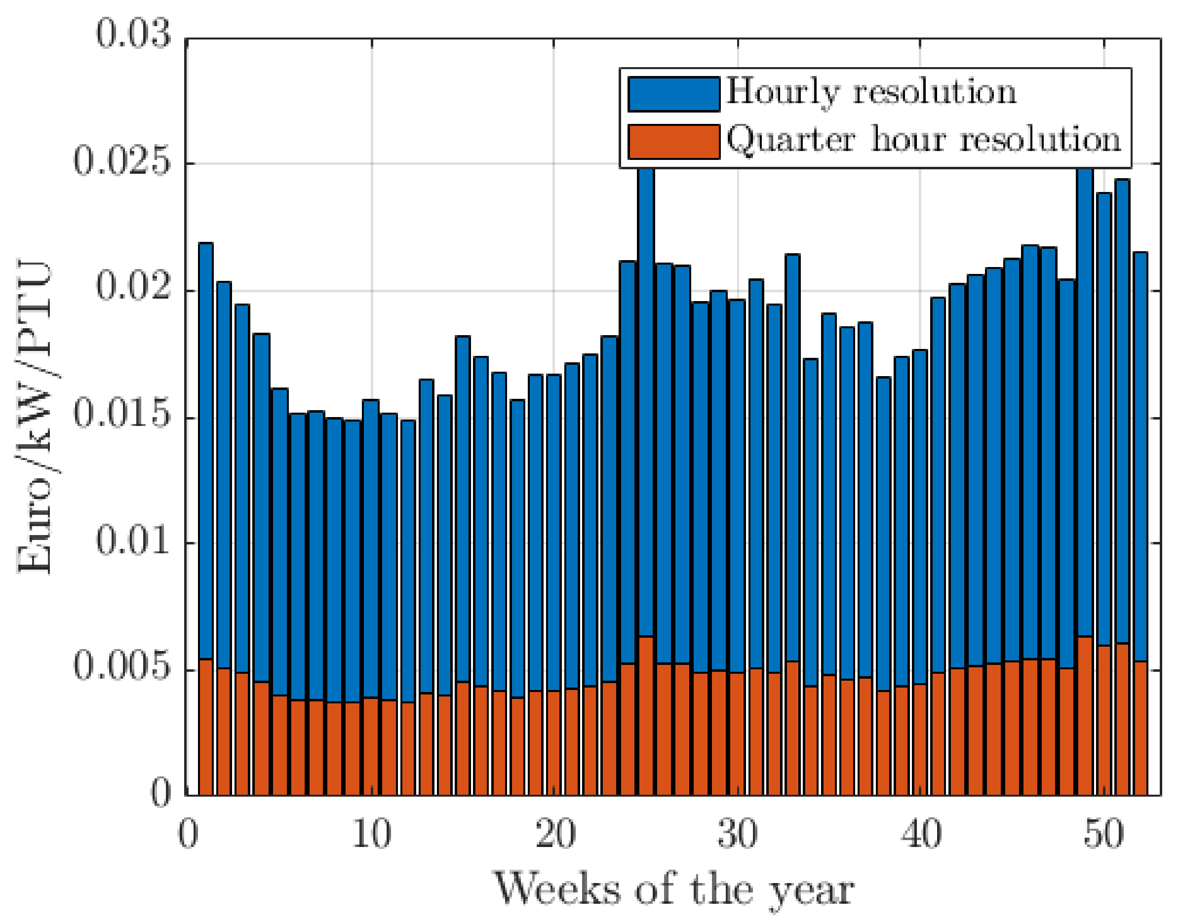
• a two-stage model predictive controller consisting of an optimal charging algorithm and real-time controller implemented in a moving horizon control scheme to compensate forecasting and estimation errors, such as PV power or SoC estimation, at a one-minute resolution. It was found that using a moving horizon window and real-time control scheme furthers reduces the costs by 9.7% compared to the reduction in cost of only optimal scheduling;
• a forecast of PV power and load demand in 15-min resolution up to 48 h ahead. Even using advanced irradiance forecasting, root mean square errors can be up to 45% [30], showing the necessity of a model predictive controller; and
• Smart grid implementation in order for the system to be integrated into a future smart grid, allowing for power curtailment and optimization of available reserved capacity for primary frequency regulation, further reducing the cost by 7.8%.

Using the above components, the actual cost of energy can be accurately assessed and minimized based on forecasts and EV/BES degradation, after which possible errors are compensated and charging can be controlled up to a resolution of one minute while taking into account ancillary services to help increase the EV and PV penetration rate.

1.3. Paper Organization

The paper is organized as follows: In Section 2, the smart charging system and its place in the smart grid paradigm will be elaborated, after which the integration of forecasts will be presented in Section 3. The control scheme will be presented in Section 4. Finally, the obtained results are presented in Section 5.

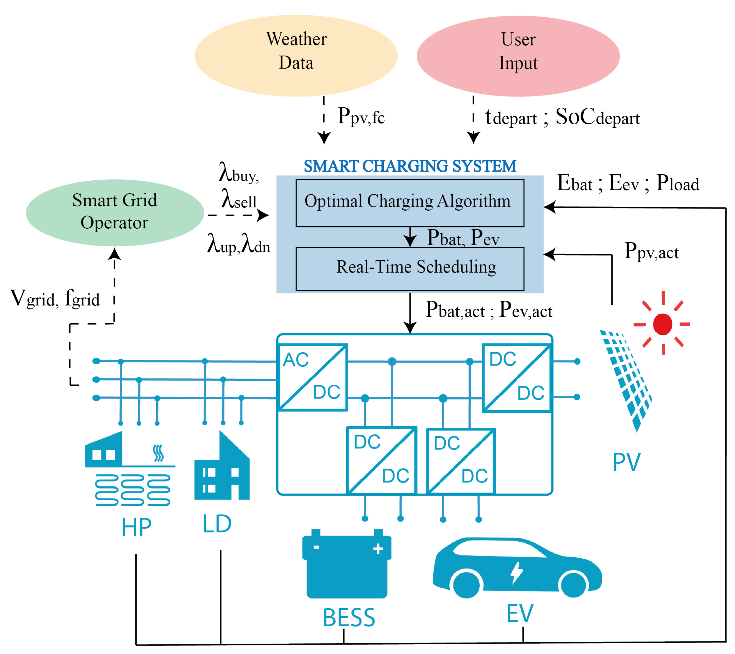
2. System Description and Smart Grid Implementation

The proposed smart charging system consists of two stages: first, an optimization algorithm finds the optimal charging strategy based on a 15-min resolution. Secondly, a real-time scheduling algorithm operates in real-time within the optimization timesteps. This is integrated into a moving horizon window used to take care of forecast and estimation errors, such as PV/load power, EV arrival times, SoC estimation, etc. The smart charging system is designed to control a multi-port power converter that integrates a PV maximum power point tracker (MPPT), bidirectional BES charger, bidirectional EV charger, and grid-connected inverter on the same DC-link [31,32]; see Figure 1. By connecting these on the same DC-link, several inverting/rectifying power steps can be omitted, achieving higher efficiency and power density. All specifications are given in

Table 1. Multi-port system parameters.

Symbol	Quantity	Value
$P_{PV}^{rated}$	installed PV capacity power	10 kWp
$P_{ev}$	Maximum EV (dis)charging power	10 kW
$P_{}$	Maximum battery (dis)charging power	10 kW
$E_{ev}$	Initial full EV capacity	80 kWh
$E_{BES}$	Initial full battery capacity	10 kWh
$V_{oc,ev}$	EV voltage	325–430 V
$V_{oc,BES}$	BES voltage	325–430 V

; the voltages of the EV and BES are based on [33,34]. Since the inverter is maintaining the power balance on the DC link, it does not require any additional setpoints from the smart charging system. Furthermore, a heat pump connects to the AC side for building heating and tap water. This study assumes that the state-of-charge (SoC) of the BES and EV are known according to the ISO 15118 standard. Finally, as part of the future smart grid, a Smart Grid Operator (SGO) is taken into account, which acts as an aggregator and intermediary between the ancillary services, wholesale market, and small-scale prosumers. This SGO provides the real-time electricity price (${\lambda }_{buy/sell}$) as well as up/downregulation prices (${\lambda }_{up/dwn}$). As a result, the smart charging algorithm can take place in regulatory services and can take this into account in the optimization. Finally, the SGO can also limit the grid power of the system as part of a demand-side management program, for which the user will be financially compensated afterwards.

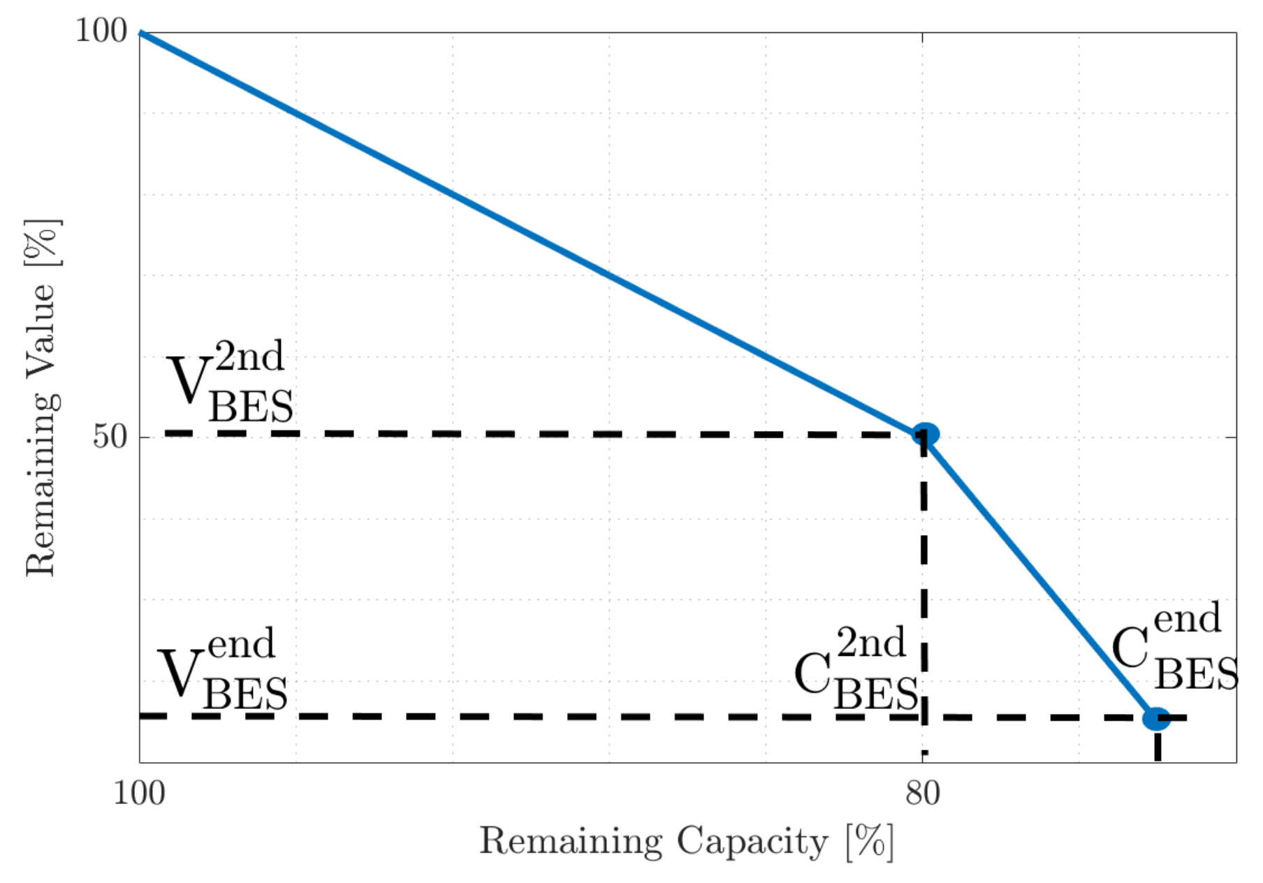
3. Second-Life Batteries

Due to the increasing amount of EVs, new markets for second-life EV batteries emerge as EV batteries often have 70–80% remaining capacity left at the end of their EV lifetime [35]. These second-life batteries are then repurposed for stationary applications such as grid reinforcement or demand response systems. This reduces the cost of EV/BES ownership as well as increases the sustainability of the Li-ion batteries. In this study, the second-life value of both the EV and the BES is taken into account and used to assess the operational costs of EV/BES ownership more accurately. Additionally, in [36], it was found that second-life battery performance and state-of-health estimation is strongly influenced by its first-life performance. This motivates the use of a battery degradation model, which minimizes and monitors the degradation such that the performance of the battery in its second-life is increased and more easily assessed.

4. Materials and Methods

The proposed smart charging algorithm can be divided into three subsection: 1. forecasting, 2. optimal scheduling, and 3. moving horizon and real-time control scheme.

4.1. Forecasting

Solar PV and load demand forecasts are required in order to schedule the charging of EV and BES accurately. The forecasting of PV energy can be divided into three categories: statistical data-based methods such as Auto Regressive Integrating Moving Average (ARIMA) [37,38] and machine learning based methods such as neural networks. The disadvantage of the methods mentioned above is that their accuracy solely relies on historical data, as there are no environmental inputs. The third category is a hybrid method based on historical data as well as weather data and satellite images. This study uses the solar radiation forecasts of the royal dutch weather institute. The advantage of this is that the computation of the forecasts is being performed outside the moving horizon controller and is based on previous data, satellite images, weather prediction modelling, and radiative transfer modelling [39]. The forecast is a combination of a short-term forecast (0–6 h) (SEVIRI) and a long-term forecast up to 48 h (HARMONIE) and includes Global Horizontal Irradiance (GHI) and Direct Normal Irradiance (DNI) [30]. In combination with the moving horizon control, good accuracy on the short term can be obtained, while at the same time, scheduling up to 48 h ahead can be performed. Then, using the approach presented in [32], the produced PV power can be calculated based on the orientation of the solar panels. Forecasting the load demand is done based on an aggregated residential profile obtained from [40]. Here, both appliance and heating demand are taken into account. An example of the forecasted and actual powers is shown in Figure 2. Even though the forecasted trend of PV power is accurate, sudden clouding can still cause significant errors of several kilowatts. Similarly, for the load demand profile, its highly stochastic nature is not captured by the aggregated data. However, daily and seasonal variations are incorporated. Due to the existence of these errors combined with a relatively coarse resolution of 15 min in most optimal scheduling problems, significant deviations from the actual optimal solution would occur. This motivates the use of a real-time control scheme.

4.2. Optimal Charging Algorithm

In this section, the optimization model is discussed. All variables are denoted and described in the nomenclature at the end of this article. The optimal charging algorithm’s goal is to find the optimal charging schedule based on the forecasts of load and PV while taking into account battery degradation and ancillary services. The main contribution of the proposed optimization problem is the use of a Li-ion battery degradation model. Because of the good balance of power density, energy density, and lifetime, Nickel-Manganese-Cobalt (NMC) based batteries are being used for both vehicle and stationary applications [41]. Therefore, the same ageing model can be used for both the stationary and vehicle battery. Similarly, the costs of V2G, regulatory services, and degradation can be determined based on the actual operating conditions. Furthermore, since the model is included in the objective, the solver will minimize the degradation and the resulting costs. The non-linear behaviour of these cells makes the optimization problem a non-linear programming (NLP) model. The problem was solved using the CONOPT solver (part of BARON/Antigone [42]) using the generic algebraic modelling system (GAMS) platform on a PC with 3.6 GHz, Intel Xeon 4 core and 16 GB RAM.

4.2.1. Objective Function

The objective of this optimization is to minimize the total cost of energy. Here, the total cost of energy $C_{total}$ is made up out of battery energy storage costs $C_{BES}$, electric vehicle costs $C_{EV}$, PV energy costs $C_{PV}$, grid energy costs $C_{grid}$, and regulatory revenue $C_{reg}$. Mathematically, this can be expressed as follows:

$$min\left(C_{total}\right)=min(C_{BES}+C_{EV}+C_{PV}+C_{grid}-C_{reg})$$

(1)

The battery costs are operational costs, which are determined by assessing the remaining value of the degraded battery. This is done by calculating the degraded capacity $\Delta E_{BES}^{tot}$ and by subtracting this from the initial capacity $E_{BES}^{max}$, both in kWh. Next, the remaining value per kWh, $V_{BES}$ in euro/kWh, is calculated according to the model presented in [43]. The decay of $V_{BES}$ versus the remaining capacity is shown in Figure 3. This study assumes that the battery is still in its first life, which ends at 80% remaining capacity, and that the value at the start of second-life $V_{BES}^{2nd}$ equals 50% of a new BES: $V_{BES}^{2nd}=0.5V_{BES}^{new}$[43]. $V_{BES}$ can than be calculated according to the formula presented in Equation (2). The costs are then equal to the difference between a new BES and the degraded BES as shown in Equation (3).

$$V_{BES}=\frac{(V_{BES}^{2nd}-V_{BES}^{new})}{0.2}\Delta E_{BES}^{tot}+V_{BES}^{new}$$

(2)

$$C_{BES}=V_{BES}^{new}{E}_{BES}^{max}-V_{BES}(E_{BES}^{max}-\Delta E_{BES}^{tot})$$

(3)

The costs related to the EV are related to the degradation costs of charging and V2G. A similar notation of variables as for the BES is used. Here, the degradation due to driving is not taken into account, as it is not under the control of the smart charging system. Furthermore, it is assumed that the 2nd life of an electric vehicle battery starts at 80% remaining capacity at 50% of its original value per kWh [43]. This is described in Equations (4) and (5).

$$V_{EV}=\frac{(V_{EV}^{2nd}-V_{EV}^{new})}{0.2}\Delta E_{EV}^{tot}+V_{EV}^{new}$$

(4)

$$C_{EV}=V_{EV}^{new}{E}_{EV}^{max}-V_{EV}(E_{EV}^{max}-\Delta E_{EV}^{tot})$$

(5)

In this study, the cost of PV energy is not assumed to be zero, to take into account the installation and investment costs of the PV system, or to simulate a contractual power purchase agreement. These costs are levelled per kWh to make them independent of the simulation time, without neglecting the related costs. Here, ${\lambda }_{PV}=0.03$ €/kWh [12] is assumed. The costs for PV energy are then determined according to the following:

$$C_{PV}=\sum _{t=1}^T{P}_{PV}\Delta t{\lambda }_{PV}$$

(6)

Here, $P_{PV}\left(t\right)$ is the generated PV power, $\Delta t$ is the simulation timestep, and ${\lambda }_{PV}$ is the levelized cost of PV energy. The next part of the objective function is the revenue obtained by acting as a frequency containment reserve (FCR) and demand-side management. Here, it is assumed that an SGO acts as an aggregator and mediator between the frequency regulation market and the prosumer, aggregating several flexible systems such that the combined power meets the minimum power requirements for the FCR market. Here, the revenue is obtained by reserving a part of the available power capacity for primary frequency regulation. The up/downregulation prices are ${\lambda }_{up}and{\lambda }_{dn}$, respectively. Based on these prices, the operational costs, and the current demand, the optimization will determine how much of the available capacity will be reserved for frequency regulation. The revenue obtained from this is calculated according to the following:

$$C_{reg}=(1-{ϵ}_{fc}){\eta }_{inv}{\eta }_{ch}\sum _{t=1}^T(P_{reg}^{up}\left(t\right){\lambda }_{up}\left(t\right)+P_{reg}^{dwn}\left(t\right){\lambda }_{dwn}\left(t\right))+C_{comp}$$

(7)

Here, ${ϵ}_{fc}$ is the maximum forecasting error; this is taken into account to limit the error between actual and reserved capacity caused by forecasting errors. Due to the moving horizon control, a good short-term accuracy can be achieved. However, as errors will still occur, compensation factor $C_{comp}$ is introduced such that any difference in revenue caused by differences in actual and reserved capacity or in scheduled and used capacity is compensated using $C_{comp}$. This makes $C_{comp}$ dependent on the bidding process in the regulation market. Therefore, it is assumed that the smart grid operator calculates this compensation factor based on the actual operation. Additionally, $C_{comp}$ could be the compensation obtained for curtailing PV power as part of demand-side management. Here, $C_{comp}$ could be equal to the curtailed energy multiplied by the energy price. Next, ${\eta }_{inv/ch}$ are the efficiencies of the inverter and BES/EV charger, respectively. Finally, $P_{reg}^{up/dwn}\left(t\right)$ are the reserved capacities for regulation. The calculation of these capacities will be explained later in Section 4.2.2.6. The final part of the objective function is the grid energy cost. In this study, a dynamic pricing tariff is used, where the selling price ${\lambda }_{sell}\left(t\right)$ is 10% lower than the buying price ${\lambda }_{buy}\left(t\right)$. This is done to simulate a future environment where electricity prices are a function of demand and supply, optimizing costs and separating buying/selling grid energy results in energy being taken out of the grid when demand and price are low while the energy fed back to the grid is fed in during a time of high demand and high price. The calculation of grid energy costs is shown in Equation (8).

$$C_{grid}=\sum _{t=1}^T{P}_{grid}^{buy}\left(t\right)\Delta t{\lambda }_{buy}\left(t\right)-\sum _{t=1}^T{P}_{grid}^{sell}\Delta t{\lambda }_{sell}\left(t\right)$$

(8)

Here, $P_{grid}^{buy/sell}\left(t\right)$ are the powers drawn and fed from the grid, respectively.

4.2.2. Constraints

4.2.2.1. Lithium-Ion Degradation Model

The battery degradation model is valid for both the EV and the BES, and therefore, the identifier $X=EV=BES$ is used. In order to calculate the capacity lost per time step ($\Delta E_X^{tot}\left(t\right)$), the battery degradation model presented in [44] is used. The model is semi-empirical based on 18650 Nickel-Manganese-Cobalt (NMC) cells. It takes into account temperature, current rate ($I_X^{cell}\left(t\right)$), and ampere-hours processed ($I_X^{cell}\left(t\right)\delta t$). In this study, the cell temperatures are assumed constant at $35{}^{\circ }$C, assuming that the EV has a battery temperature control system and because the inside ambient temperature setpoint of the heat pump varies between ${18}^{\circ }$ and 20.5 ${}^{\circ }$C [45]. A distinction between cyclic and calendar ageing is made, denoted as $\Delta E_X^{cycle}\left(t\right)$ and $\Delta E_X^{cal}\left(t\right)$. Since calendar ageing is mostly dependent on time and temperature [44] and cell temperature is assumed constant, the equation can be simplified to a constant degradation per time step. Here, a minimum lifetime of 5 years is assumed. This is shown in Equation (12).Furthermore, the model is based on the behaviour of a single cell. Therefore the EV/BES power needs to be scaled into the voltage and current of a single cell. To do this, the open-circuit voltage of an NMC cell is used, which can be described by the curve fitted equation shown in Equation (9) [46]. Here, $So{C}_x\left(t\right)$ denotes the state of charge of x at time t. The resulting curve is shown in Figure 4. Furthermore, it is assumed that $N_X^{parallel}$ by $N_X^{series}$ of these cells are placed in parallel and series respectively, such that the total open-circuit voltage $V_{oc,X}$ resembles existing EV/BES systems [33,34].

$$V_{oc,X}\left(t\right)=N_X^{series}(a_1{e}^{b_{1}So{C}_x\left(t\right)}+a_2{e}^{b_{2}So{C}_x\left(t\right)}+a_{3}So{C}_x{\left(t\right)}^2),\forall t$$

(9)

$$i_X^{cell}\left(t\right)=\frac{P_X\left(t\right)}{N_X^{parallel}{V}_{oc,X}\left(t\right)},\forall t$$

(10)

Then, using the calculated cell voltage and current from Equation (9) and (10), the lost capacity per cell can be calculated according to Equations (11) and (13) [44]. Note that the model presented in [44] calculates the percentage of lost charge in ampere hour and is therefore multiplied with $\frac{E_{BES}^{max}}{100}$ in order to get the actually lost capacity. The values of the curve fitted parameters in Equations (9)–(13) can be found in

Table 2. Battery model parameters.

Symbol	Quantity	Value
$N_{cell}^{parallel}$	Number of battery cells in parallel	14
$N_{cell}^{series}$	Number of battery cells in series	100
$a_1$	$V_{oc}\left(t\right)$ curve fit parameter	3.679
$b_1$	$V_{oc}\left(t\right)$ curve fit parameter	−0.1101
$a_2$	$V_{oc}\left(t\right)$ curve fit parameter	−0.2528
$b_2$	$V_{oc}\left(t\right)$ curve fit parameter	−6.829
$a_3$	$V_{oc}\left(t\right)$ curve fit parameter	0.9386
$c_1$	ageing curve fit parameter	0.00054
$c_2$	ageing curve fit parameter	0.35
$c_3$	ageing curve fit parameter	14,876
$c_4$	averaged calendar ageing per $\Delta t$	2.64 × 10${}^{-4}$

.

$$\Delta E_X^{cycle}\left(t\right)=(c_1{e}^{c_2\left|i_X^{cell}\left(t\right)\right|}\left|i_X^{cell}\left(t\right)\right|\Delta t)\frac{E_{BES}^{max}}{100},\forall t$$

(11)

$$\Delta E_X^{cal}\left(t\right)=\left(c_3\sqrt{t}{e}^{-24kJ/RT}\right)\frac{E_{BES}^{max}}{100}=(c_4\Delta t)\frac{E_{BES}^{max}}{100},\forall t$$

(12)

$$\Delta E_X^{tot}=\sum _{t=0}^T(\Delta E_X^{cycle}\left(t\right)+\Delta E_X^{cal}\left(t\right))$$

(13)

4.2.2.2. Battery Energy Storage Constraints

The BES power $P_{BES}\left(t\right)$ is limited between [−10, 10] kW. Additionally, the maximum power $P_{BES}^{max}\left(t\right)$ is SoC dependent such that the maximum power drops linearly below a SoC of 10% ($D_{dis}=0.1$) and above a SoC of 80% ($D_{ch}=0.8$), representing the constant-current constant-voltage regions of a battery. This is ensured using Equations (14)–(20). The round-trip efficiency is considered constant over power and lifetime and is equal to 95 % [34]. Therefore, the efficiency of a single charge/discharge cycle equals ${\eta }_{ch/dis}=\sqrt{0.95}=0.975$. Due to this efficiency, the model recognizes the loss of energy and therefore prevents both $P_{BES}^{neg}\left(t\right)$ and $P_{BES}^{pos}\left(t\right)$ from having nonzero values at the same time.

$$P_{BES}^{pos}\left(t\right)\le P_{BES}^{max}\left(t\right),\forall t$$

(14)

$$P_{BES}^{max}\left(t\right)\le P_{BES}^{rated}\left(t\right),\forall t$$

(15)

$$P_{BES}^{max}\left(t\right)\le \frac{P_{BES}^{max}}{1-D_{ch}}(\frac{E_{BES}\left(t\right)}{E_{BES}^{max}}-1),\forall t$$

(16)

$$P_{BES}^{neg}\left(t\right)\le P_{BES}^{min}\left(t\right),\forall t$$

(17)

$$P_{BES}^{min}\left(t\right)\le P_{BES}^{rated},\forall t$$

(18)

$$P_{BES}^{min}\left(t\right)\le \frac{P_{BES}^{rated}}{D_{dis}}\frac{E_{BES}\left(t\right)}{E_{BES}^{max}},\forall t$$

(19)

$$P_{BES}\left(t\right)={\eta }_{ch}{P}_{BES}^{pos}\left(t\right)-\frac{1}{{\eta }_{dis}}{P}_{BES}^{neg}\left(t\right),\forall t$$

(20)

In the above constraints as well as all the following constraints, the superscripts “max”, “min”, “pos”, “neg”, and “rated” declare the maximum allowable, minimum allowable, actual positive, actual negative, and rated powers.The energy stored inside the BES $E_{BES}\left(t\right)$ can then be calculated according to Equation (21). Here, the BES capacity is fixed for $t=1$ and $t=t_{final}$ at capacities $E_{BES}^{init}=E_{BES}^{final}$, respectively, in order to have a fair comparison between costs.

$$E_{BES}\left(t\right)=\left\{\begin{array}{cc}{E}_{BES}^{init},\hfill & \mathrm{for}t=1\hfill \\ E_{BES}(t-1)+P_{BES}\left(t\right)\Delta t,\hfill & \mathrm{for}1<t<t_{final}\hfill \\ E_{BES}^{final},\hfill & \mathrm{for}t=t_{final}\hfill \end{array}\right.$$

(21)

Furthermore, the SoC of the BES is calculated using Equation (22). Here, $E_{BES}^{limit}\left(t\right)$ is a variable which represents the actual maximum capacity at time t, which equals the initial maximum capacity $E_{BES}^{max}$ minus the capacity lost by cycling for that time step $\Delta E_{BES}\left(t\right)$. This is modelled using Equation (23) and Equation (24).

$$So{C}_{BES}\left(t\right)=\frac{E_{BES}\left(t\right)}{E_{BES}^{limit}\left(t\right)},\forall t$$

(22)

$$E_{BES}^{limit}\left(t\right)=\left\{\begin{array}{cc}{E}_{BES}^{max},\hfill & \mathrm{for}t=1\hfill \\ E_{BES}^{limit}(t-1)-\Delta E_{BES}\left(t\right),\hfill & \mathrm{for}t>1\hfill \end{array}\right.$$

(23)

$$E_{BES}\left(t\right)\le E_{BES}^{limit}\left(t\right),\forall t$$

(24)

4.2.2.3. Electric Vehicle Constraints

The electric vehicle constraints are given in Equations (25)–(36), where the constraints up to Equation (34) are similar to the BES constraints. The electric vehicle is assumed to be unavailable from $t_{depart}$ = 08:00 till $t_{arrive}$ = 18:00 during the day; this is denoted by the binary parameter $E{V}_{av}\left(t\right)$, which equals 0 for $t_{depart}\le t\le t_{arrive}$. These departure and arrival times are based on the distribution, as presented in [47]. During that time, it is estimated that the EV is commuting between work and home, where a single trip is 30 km with an efficiency of 15 kWh/100 km [48], resulting in a 9 kWh decrease in charge at arrival; note that the arrival time and charge are only estimations and that possible errors will be compensated after arrival as a result of the moving horizon window.

$$P_{EV}^{pos}\left(t\right)\le P_{EV}^{max}\left(t\right),\forall t$$

(25)

$$P_{EV}^{max}\left(t\right)\le P_{EV}^{rated}\left(t\right),\forall t$$

(26)

$$P_{EV}^{max}\left(t\right)\le \frac{P_{EV}^{max}}{1-D_{ch}}(\frac{E_{EV}\left(t\right)}{E_{EV}^{max}}-1),\forall t$$

(27)

$$P_{EV}^{neg}\left(t\right)\le P_{EV}^{min}\left(t\right),\forall t$$

(28)

$$P_{EV}^{min}\left(t\right)\le P_{EV}^{rated},\forall t$$

(29)

$$P_{EV}^{min}\left(t\right)\le \frac{P_{EV}^{rated}}{D_{dis}}\frac{E_{EV}\left(t\right)}{E_{EV}^{max}},\forall t$$

(30)

$$P_{EV}\left(t\right)=E{V}_{av}\left(t\right)({\eta }_{ch}{P}_{EV}^{pos}\left(t\right)-\frac{1}{{\eta }_{dis}}{P}_{EV}^{neg}\left(t\right)),\forall t$$

(31)

$$So{C}_{EV}\left(t\right)=\frac{E_{EV}\left(t\right)}{E_{EV}^{limit}\left(t\right)},\forall t$$

(32)

$$E_{EV}^{limit}\left(t\right)=\left\{\begin{array}{c}{E}_{EV}^{max},\mathrm{for}t=1\hfill \\ E_{EV}^{limit}(t-1)-\Delta E_{EV}\left(t\right),\mathrm{for}t>1\hfill \end{array}\right.$$

(33)

$$E_{EV}\left(t\right)\le E_{EV}^{limit}\left(t\right),\forall t$$

(34)

Finally, the user can state a minimum departure charge $E_{depart}$ and departure time $t_{depart}$, which ensures that the EV always has enough charge at the time of departure. This is modeled using Equation (36):

$$E_{EV}\left(t\right)=\left\{\begin{array}{cc}{E}_{EV}^{init},\hfill & \mathrm{for}t=1\hfill \\ E_{EV}(t-1)+P_{EV}\left(t\right)\Delta t,\hfill & \mathrm{for}t\le t_{depart}\hfill \\ \hfill & \&t\le t_{depart}\hfill \end{array}\right.$$

(35)

$$E_{EV}\left(t\right)\ge E_{EV}^{depart},\mathrm{for}t=t_{depart}$$

(36)

4.2.2.4. Power Balance Constraints

For the given system (Figure 1), two power balances exist: 1. on the DC link of the multi-port converter. Here, a positive inverter power $P_{inv}\left(t\right)$ equals feeding power to the grid. 2. The second power balance exists on the AC side between the inverter and the meter. This is modeled using Equations (37) and (38).

$$P_{inv}\left(t\right)=P_{PV}\left(t\right)-P_{BES}\left(t\right)-P_{EV}\left(t\right),\forall t$$

(37)

$$P_{grid}\left(t\right)={\eta }_{inv}{P}_{inv}\left(t\right)-P_{load}\left(t\right),\forall t$$

(38)

Here, the total load $P_{load}\left(t\right)$ consists of the load from all appliances in the building $P_{appl}\left(t\right)$ and the power required for heating $P_{heat}\left(t\right)$, in the form of a heat pump. In this study, both $P_{appl}\left(t\right)$ and $P_{heat}\left(t\right)$ are considered non-flexible.

$$P_{load}\left(t\right)=P_{appl}\left(t\right)+P_{heat}\left(t\right),\forall t$$

(39)

4.2.2.5. Grid Constraints

The resulting grid power $P_{grid}\left(t\right)$ differentiates between positive and negative grid powers since both have different prices. This is done using the efficiency ${\eta }_{cable}$, which models the power loss in the cable between the meter and converter. This efficiency is assumed to equal 99%. However, more importantly, it ensures that the $P_{grid}^{buy}\left(t\right)$ and $P_{grid}^{sell}\left(t\right)$ do not have nonzero values simultaneously, as the efficiency loss is recognized. This allows for grid power arbitration without the use of binary variables, drastically increasing the solving time. Here, $P_{grid}^{max}$ is the maximum power of a 3-phase 25A connection.

$$P_{grid}^{sell}\left(t\right)\le P_{grid}^{max},\forall t$$

(40)

$$P_{grid}^{buy}\left(t\right)\le P_{grid}^{max},\forall t$$

(41)

$$P_{grid}\left(t\right)={\eta }_{cable}{P}_{grid}^{sell}\left(t\right)-\frac{1}{{\eta }_{cable}}{P}_{grid}^{buy}\left(t\right),\forall t$$

(42)

4.2.2.6. Regulation Market Constraints

Part of the objective function is the revenue obtained from reserving the capacity for primary frequency regulation. Here, it is assumed that the system is part of a smart grid as described in Section 2. Using Equations (43)–(47), it is ensured that the maximum available capacity for regulation does not exceed the actual maximum capacity in the system. Here, it is important to note that the maximum available EV/BES capacity is SoC dependent. Therefore, the available up/down capacity per converter port $P_{up/dwn}^x\left(t\right)$ (x = EV/BES/PV) is denoted using $P_x^{max/min}\left(t\right)$, as calculated in Section 4.2.2.2 and Section 4.2.2.3. Similarly, it has been done for down regulation in Equations (48)–(53).

$$P_{up}^{EV}\left(t\right)\le E{V}_{av}\left(t\right)(P_{EV}^{min}\left(t\right)+P_{EV}\left(t\right)),\forall t$$

(43)

$$P_{up}^{BES}\left(t\right)\le P_{BES}^{min}\left(t\right)+P_{BES}\left(t\right),\forall t$$

(44)

$$P_{up}\left(t\right)\le {\eta }_{inv}(P_{up}^{EV}\left(t\right)+P_{up}^{BES}\left(t\right)),\forall t$$

(45)

$$P_{up}\left(t\right)\le P_{inv}^{rated}\left(t\right),\forall t$$

(46)

$$P_{up}\left(t\right)\le P_{grid}^{max}\left(t\right)+P_{load}\left(t\right),\forall t$$

(47)

$$P_{dwn}^{EV}\left(t\right)\le E{V}_{av}\left(t\right)(P_{EV}^{max}\left(t\right)-P_{EV}\left(t\right)),\forall t$$

(48)

$$P_{dwn}^{BES}\left(t\right)\le P_{BES}^{min}\left(t\right)-P_{BES}\left(t\right),\forall t$$

(49)

$$P_{dwn}^{PV}\left(t\right)\le P_{PV}\left(t\right),\forall t$$

(50)

$$P_{dwn}\left(t\right)\le {\eta }_{inv}(P_{EV}^{dwn}\left(t\right)+P_{BES}^{dwn}\left(t\right)+P_{PV}^{dwn}\left(t\right)),\forall t$$

(51)

$$P_{dwn}\left(t\right)\le P_{inv}^{rated}\left(t\right),\forall t$$

(52)

$$P_{dwn}\left(t\right)\le P_{grid}^{max}\left(t\right),\forall t$$

(53)

In case of symmetric reserve offers, Equation (54) should also be used.

$$P_{up}\left(t\right)=P_{dwn}\left(t\right),\forall t$$

(54)

4.2.2.7. Inverter Constraints

To account for the efficiency of the inverter, the inverter power is also split into positive and negative parts. The inverter efficiency is assumed equal for both directions of power: 97% and over the entire power range [24].

$$P_{inv}^{neg}\left(t\right)\le P_{inv}^{max},\forall t$$

(55)

$$P_{inv}^{pos}\left(t\right)\le P_{inv}^{max},\forall t$$

(56)

$$P_{inv}\left(t\right)={\eta }_{inv}{P}_{inv}^{pos}\left(t\right)-\frac{1}{{\eta }_{inv}}{P}_{inv}^{neg}\left(t\right),\forall t$$

(57)

4.2.2.8. Photovoltaic Constraints

As part of demand-side management as well as for cases with a negative feed-in tariff, it should be possible to curtail PV power. Therefore, in order to allow PV power curtailment, Equation (58) is introduced. Here, the efficiency of the maximum power point tracker is assumed to be ${\eta }_{mppt}=98\%$ [49]. Here, $P_{PV}^{forecast}\left(t\right)$ denotes the forecasted PV power. This concludes the optimization model section. In the next section, the proposed real-time control is discussed.

$$P_{PV}\left(t\right)\le {\eta }_{mppt}{P}_{PV}^{forecast}\left(t\right),\forall t$$

(58)

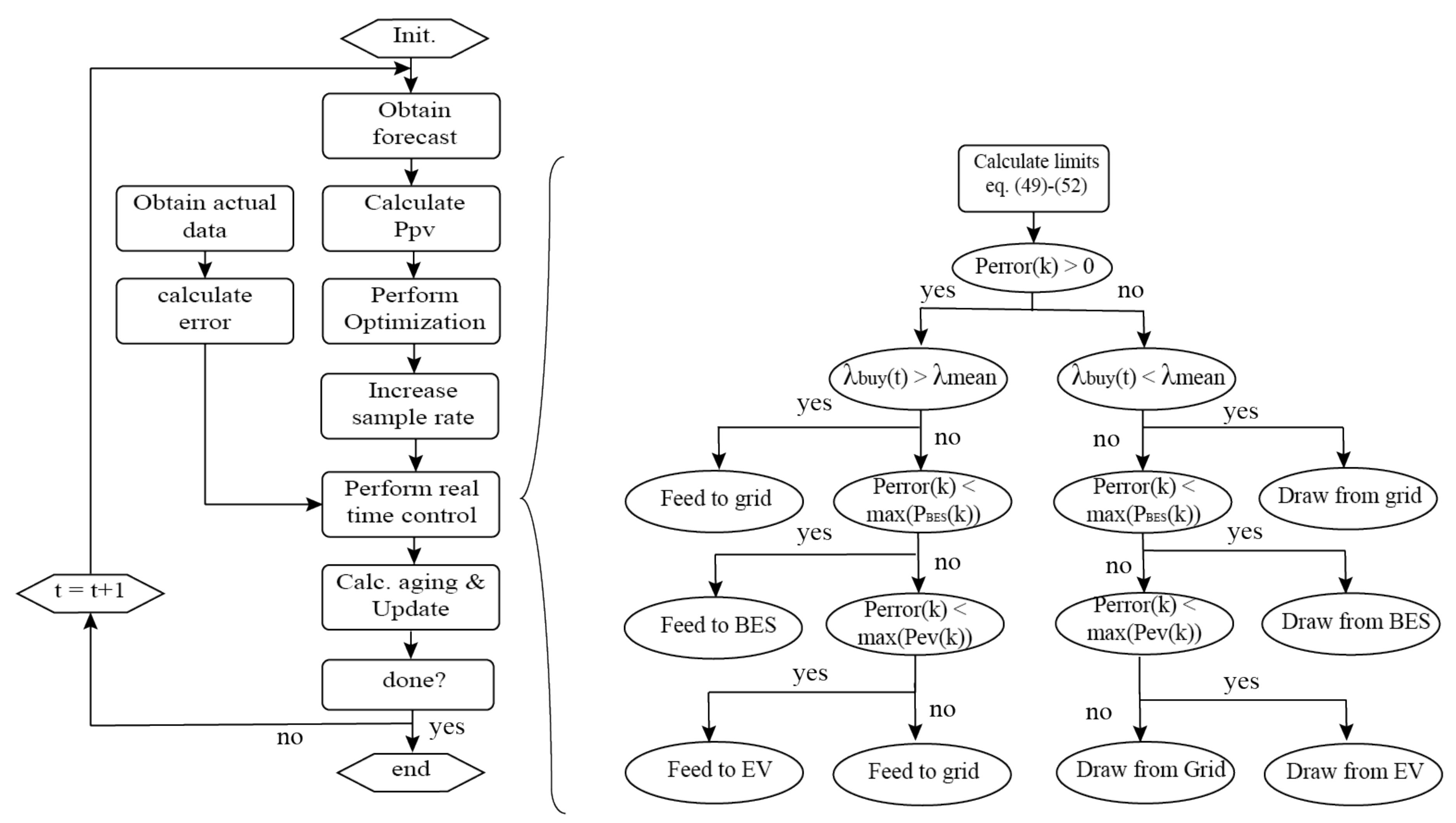
4.3. Moving Horizon Window and Real-Time Control

In Section 4.2, the optimal charging algorithm is discussed. The goal of the optimal charging algorithm is to find the optimal charging schedule within a 24-h optimization window while anticipating future demand and supply based on forecasts and taking into account battery degradation, and primary frequency regulation reserve. However, as shown in Figure 2, the resulting forecasting errors can still be in the range of several kWs. To minimize the effect of these errors, a moving horizon model predictive controller is implemented, which reoptimizes every 15 min (i.e., one optimization timestep). Additionally, a new forecast is obtained every hour to improve accuracy. To compensate for the errors within these 15-min timesteps, such as PV power, SoC estimation, and EV time of arrival, a real-time control scheme is implemented. Here, a rule-based control scheme is implemented such that it can act almost instantly. It should be noted that the real-time control only deals with the errors on top of what is optimally scheduled. For example, if the battery is directly charging from PV power in the optimal solution but the PV power turns out to be less than forecasted, the battery power can be changed accordingly. If no real-time control is implemented, this error needs to be compensated using grid power to maintain the power balance on the DC-link inside the multi-port converter, which could lead to nonoptimal solutions. Figure 5 shows the flowchart of the moving horizon control and the real-time control scheme. First, the irradiance forecasts are obtained, and the resulting PV power is calculated. Then, after the optimization, the output at t = 1 is saved and the sample rate is increased 15 times, such that the resolution is now one minute. The interpolated variables are indicated with index k. Furthermore, superscripts $fc$ and $act$ denote the forecasted and actual powers, respectively. In practice, the resolution can be as small as computation time allows to get actual real-time operation. The new real-time charging schedule is determined based on the amplitude of the error, the available EV/BES power, and the current electricity price. The error is calculated according to Equations (59)–(61).

$$\Delta P_{PV}\left(k\right)=P_{PV}^{fc}\left(k\right)-P_{PV}^{act}\left(k\right)$$

(59)

$$\Delta P_{load}\left(k\right)=P_{load}^{fc}\left(k\right)-P_{load}^{act}\left(k\right)$$

(60)

$$P_{error}\left(k\right)=\Delta P_{load}\left(k\right)-\Delta P_{PV}\left(k\right)$$

(61)

Here, a positive error means an excess of power. For example, when the actual PV power is higher as forecasted (i.e., $\Delta P_{PV}\left(k\right)>0$) while the actual load is lower as anticipated (i.e., $\Delta P_{load}\left(k\right)<0$), the resulting error is positive $P_{error}\left(k\right)>0$. Next, the power limitations of the EV/BES converter at time k are determined based on power rating, SoC, and power balance inside the multi-port system. This is done using Equations (62)–(65). A rule-based control scheme then determines how the error should be compensated based on $P_{error}$, the power limitations, current electricity price, and the mean electricity price calculated according to Equation (66), as shown in Figure 5. The goal of the real-time control scheme is to prevent feeding in power to the grid at times of low electricity prices or drawing power during high electricity prices. For example, when the error is positive (meaning an excess of power) and the electricity price ${\lambda }_{buy}$ is above average (${\lambda }_{mean}$), the power is fed to the grid. If the price would be below average, the control first checks whether the BES can absorb the power and, if not, whether the EV can absorb the power; if both are not able to absorb the excess power, it is fed to the grid. After the real-time powers have been calculated, the actual degradation is calculated and the corresponding variables are adjusted. This will then be used for initializing the next optimization instance.

$$P_{BES}^{max,neg}\left(k\right)=\max (0,\min (P_{BES}^{max},\frac{E_{BES}(k)-E_{BES}^{min}}{\Delta k},P_{inv}^{max}-P_{PV}(k)+P_{EV}(k)))$$

(62)

$$P_{BES}^{max,pos}\left(k\right)=\max (0,\min (P_{BES}^{min},\frac{E_{BES}^{max}-E_{BES}(k)}{\Delta k},P_{inv}^{max}+P_{PV}(k)-P_{EV}(k)))$$

(63)

$$P_{EV}^{max,neg}(k)=\max (0,\min (P_{EV}^{max},\frac{E_{EV}(k)-E_{EV}^{min}}{\Delta k},P_{inv}^{max}-P_{PV}(k)+P_{BES}(k)))$$

(64)

$$P_{EV}^{max,pos}\left(k\right)=\max (0,\min (P_{EV}^{min},\frac{E_{EV}^{max}-E_{EV}(k)}{\Delta k},P_{inv}^{max}+P_{PV}(k)-P_{BES}(k)))$$

(65)

$${\lambda }_{mean}=\frac{{\sum }_{t=t}^{t=T}{\lambda }_{buy}\left(t\right)}{T},T\in [t,t+24h]$$

(66)

5. Use Case and Price Mechanism

The system specifications can be found in Table 1 above. The proposed optimal control scheme can be applied to any building with an EV, solar panels, heat pump, and BES. In this study, a residential building has been chosen as a use case. The building appliance load is obtained from a Dutch distribution system operator and represents a building with a medium to high demand. Both heating and appliance loads are assumed to be non-flexible such that no compromise is given to the user. The power profile of the heat pump is interpolated hourly data obtained from a study performed by the Dutch Organization for Applied Scientific Research [45]. Here, a medium isolated residential building is used with an inside temperature setpoint that varies between $18{}^{\circ }$C and $20.5{}^{\circ }$C during night and day, respectively. It is assumed that a time-varying electricity price is obtained from the SGO. The price signal is equal to the Amsterdam Power Exchange market [38,50] only averaged around 0.20 €/kWh, see Figure 6. Additionally, up/downregulation prices ${\lambda }_{up/down}$ are obtained from the SGO and shown in Figure 7. The model has been formulated such that it can operate with any kind of regulation market. In this case, the German primary frequency control market was chosen because it resembles the Dutch frequency control market. The German Frequency Regulation market is a symmetrical market, so both up- and downregulation are equally priced. Figure 7 displays the prices obtained for every week in 2018 [51].

6. Results and Discussion

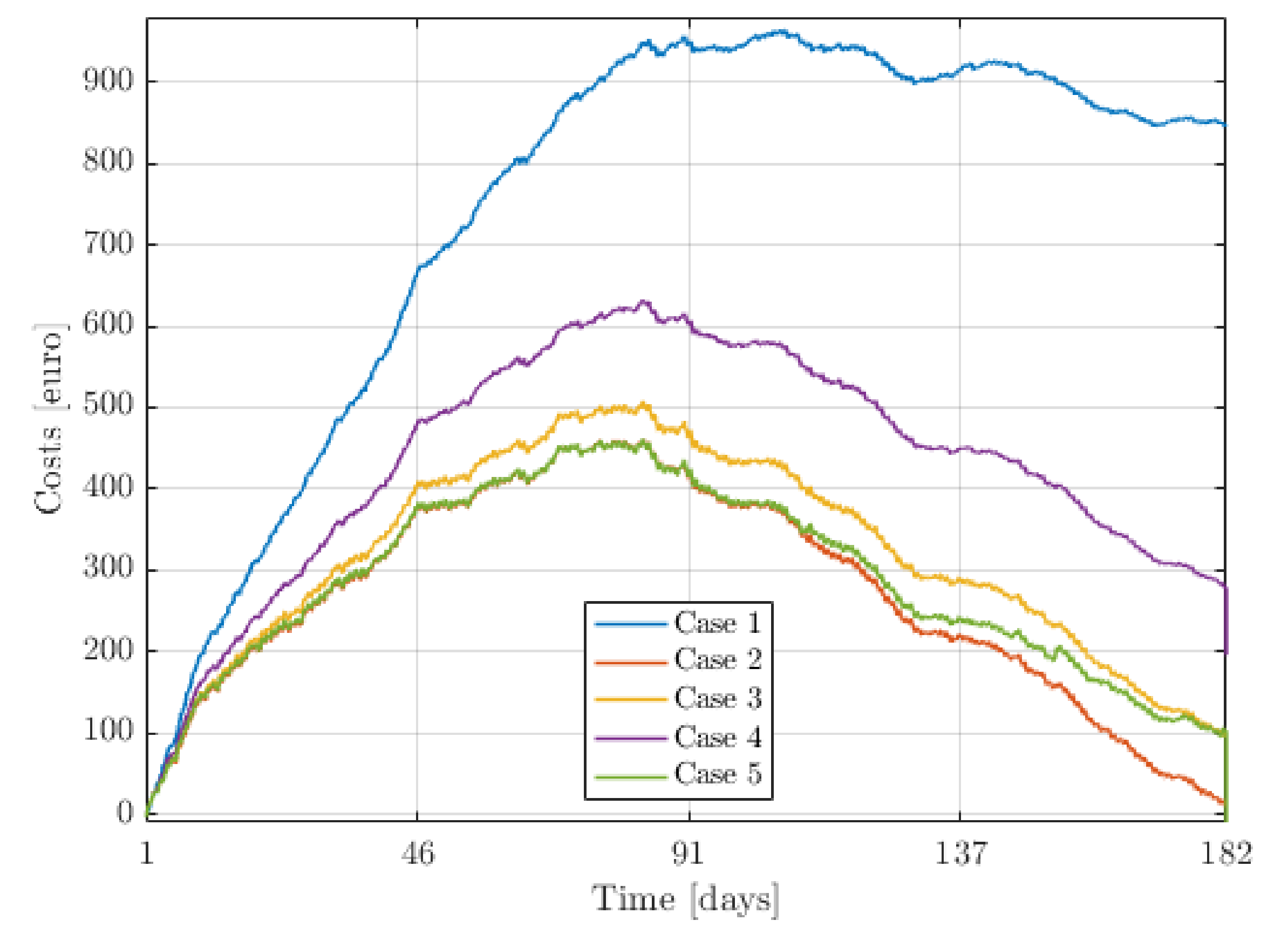
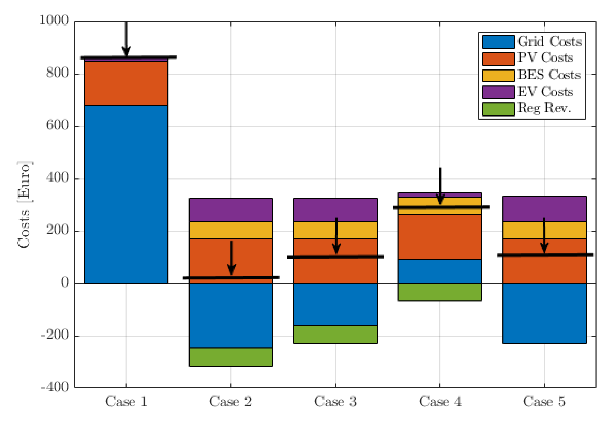
The results for summer and winter days are shown in Figure 8, Figure 9, Figure 10 and Figure 11, respectively. Here, the electricity buying price and forecasted and actual PV/load powers are included as well. From both Figure 8 and Figure 10, it is clear that the optimal charging stage trades energy in between times of high and low prices. Similarly, it decides when to store PV energy and when to feed it back to the grid. During winter, the energy demand is much higher, mainly because of the increased heating demand. Additionally, the PV production is much lower and, therefore, less energy is fed to the grid. Without an appropriate control scheme, the BES would only be used in case of excess PV energy, therefore resulting in poor utilization of the BES. However, the proposed model still fully utilizes the available BES capacity in order to reduce the cost of energy. This is also shown in Figure 9 and Figure 11. The EV is charged at night above the required departure charge of 50 kWh, such that it can utilize V2G when prices are high in the morning and again in the evening up to the point where prices are low again at the end of the day. Note that the usable EV capacity is not completely utilized, as the inverter power rating limits the possible power exchanged with the grid, whereas outside the instances of peak/valley prices, the difference between feed-in and retail price is probably not enough to overcome the additional losses caused by the degradation of charging at higher powers. The role of the real-time control scheme can be seen in Figure 8; as PV forecasting errors occur, the algorithm decides whether to use the BES, EV, or grid to compensate for these errors. The grid is used for positive errors (excess of power) and high prices, while the BES/EV is used when errors are positive but prices are low (if possible to store energy) and vice versa for high prices and negative errors. Finally, the effect of the degradation model is seen by the peak powers of the EV/BES. Both are rated at 10 kW. However, their powers only exceed the [−6 kW, 6 kW] range at 3.44% of the time (at 1-min resolution).

6.1. Comparison

From the literature review presented above, it can be concluded that most of the existing studies only discuss the optimal scheduling of EV/BES charging. However, within a 15-min forecasting resolution, large forecasting errors can occur due to the fast changing intermittent character of PV power. Additionally, other estimations such as $t_{arrival}$ can lead to more errors. Therefore, a moving horizon window including real-time control scheme is an important part for a smart charging algorithm, as errors are compensated and the optimization is iterated. In order to assess the effectiveness of all the different components, several case studies are performed over a half-year period:

• case 1: Uncontrolled case (only EV, PV, and load)
• case 2: Proposed optimal and real-time control scheme
• case 3: Proposed optimal control and error compensation using grid power
• case 4: Proposed optimal and real-time control scheme without V2G.
• case 5: Proposed optimal and real-time control scheme without up/downregulation.

Here, it is assumed that a half-year simulation period is enough to capture all seasonal variations and that the forecasting error ${ϵ}_{fc}=0$ in order to assess the maximal potential of acting as a FCR. Furthermore, the moving horizon control will operate with a 24-h window in a 15-min resolution. The first uncontrolled case consists only of a PV installation, EV charger, and load. Here, it is assumed that the EV starts charging upon arrival with a 3 kW charger for 3 h to meet its daily demand. The second case is the complete proposed control scheme. The third case is similar to having only an optimal scheduling algorithm; here, all deviations from the obtained optimal solution are compensated using grid energy. The fourth case does not utilize V2G, and the fifth case does not take into account a primary frequency regulation reserve revenue. Figure 12 shows the resulting grid power for use case 2 and 3. Here, case 3 is comparable with having only an optimal control scheme (no real-time control). It can be seen that the errors are dealt with differently, in the end, increasing costs. In Figure 13, the total cumulative costs for every use case over a half year period is shown. Using the proposed control scheme (case 2), the total costs can be reduced by 98.6% compared to the uncontrolled case.

A breakdown of all cost components is shown in Figure 14 and

Table 3. Cost comparison of the presented 5 use cases.

Use Case	${\mathit{C}}_{\mathbf{grid}}$ [€]	${\mathit{C}}_{\mathbf{PV}}$ [€]	${\mathit{C}}_{\mathbf{BES}}$ [€]	${\mathit{C}}_{\mathbf{EV}}$ [€]	${\mathit{C}}_{\mathbf{Reg}}$ [€]	${\mathit{C}}_{\mathbf{Total}}$ [€]
1	679.5	169.14	0	10.38	0	859.01
2	−247.27	169.14	64.61	91.88	−66.74	11.76
3	−163.09	169.14	64.34	91.7	−66.74	95.24
4	93.4	169.14	65.68	16.94	−66.83	278.3
5	−230.74	169.14	65.54	98.367	0	102.3

. Here, it can be seen that the optimized EV and BES degradation costs for case 2 are still equal to 91.87 euro and 64.6 euro, respectively. Similarly, the total cost of PV energy equals 168.15 euro. From this, it can be concluded that all these costs are a nonnegligible part of an objective function when minimizing the total cost of energy in an EV-PV-BES-HP system. However, although these costs are relatively high, from Figure 13 and Table 3, it can be concluded that V2G still is a cost-effective method for storing renewable and demand-side management, as the revenue obtained from trading energy exceeds the costs of degradation. Furthermore, it can be seen that the EV charging costs of case 1 are actually the lowest. This is because the average charging power for case 1 is lower compared to the other cases, resulting in lower degradation, however, resulting in more grid electricity costs.

Demand-Side Management: Power Curtailment

Besides operating as a primary frequency regulation reserve, the smart charging algorithm is also capable of power curtailment. For example, when the smart grid operator foresees an over-voltage occurring in the near future, it can choose to limit the grid feed-in power of the system. An example of this is shown in Figure 15. Here, the SGO reduces the maximum allowable feed-in power to 5 kW between 09:30 and 18:00. A comparison with the same day without power curtailment is shown in Figure 16.

7. Conclusions

In this paper, a building smart charging algorithm was presented for a multi-port system integrating EV, PV, BES, and a HP. Here, the HP and appliance load were assumed fixed. Then, based on forecasts of PV production and load, the smart charging algorithm minimizes the total cost of energy incorporating grid electricity costs, PV investment and installation costs, EV/BES operational costs, and revenue obtained from operating as primary frequency regulation reserve. It has been shown that the proposed algorithm is very effective as it reduced 98.6% of the total cost of energy compared to an uncontrolled EV-PV-HP case. Additionally, the potential of V2G and the importance of forecasting error handling using a real-time moving horizon control scheme are discussed. Finally, it has been shown that EV/BES degradation costs as well as PV investment/installation costs are nonnegligible parts of an objective function which tries to minimize the total cost of energy in an EV-PV-BES-HP system.

References

1. Global Transportation Energy Consumption: Examination of Scenarios to 2040 Using ITEDD. Available online: https://www.eia.gov/analysis/studies/transportation/scenarios/pdf/globaltransportation.pdf (accessed on 7 April 2020).
2. Kempton, W.; Tomić, J. Vehicle-to-grid power implementation: From stabilizing the grid to supporting large-scale renewable energy. J. Power Sources 2005, 144, 280–294. [Google Scholar] [CrossRef]
3. Birnie, D.P. Solar-to-vehicle (S2V) systems for powering commuters of the future. J. Power Sources 2009, 186, 539–542. [Google Scholar] [CrossRef]
4. haikh, P.H.; Nor, N.B.M.; Nallagownden, P.; Elamvazuthi, I.; Ibrahim, T. A review on optimized control systems for building energy and comfort management of smart sustainable buildings. Renew. Sustain. Energy Rev. 2014, 34, 409–429. [Google Scholar] [CrossRef]
5. Cao, X.; Dai, X.; Liu, J. Building Energy-Consumption Status Worldwide and the State-of-the-Art Technologies for Zero-Energy Buildings during the Past Decade. Energy Build. 2016, 128, 198–213. [Google Scholar] [CrossRef]
6. Teleke, S.; Baran, M.E.; Bhattacharya, S.; Huang, A.Q. Rule-Based Control of Battery Energy Storage for Dispatching Intermittent Renewable Sources. IEEE Trans. Sustain. Energy 2010, 1, 117–124. [Google Scholar] [CrossRef]
7. Doukas, H.; Patlitzianas, K.D.; Iatropoulos, K.; Psarras, J. Intelligent building energy management system using rule sets. Build. Environ. 2007, 42, 3562–3569. [Google Scholar] [CrossRef]
8. Wi, Y.-M.; Lee, J.-U.; Joo, S.-K. Electric vehicle charging method for smart homes/buildings with a photovoltaic system. IEEE Trans. Consum. Electron. 2013, 59, 323–328. [Google Scholar] [CrossRef]
9. Brahman, F.; Honarmand, M.; Jadid, S. Optimal electrical and thermal energy management of a residential energy hub, integrating demand response and energy storage system. Energy Build. 2015, 90, 65–75. [Google Scholar] [CrossRef]
10. Bozchalui, M.C.; Hashmi, S.A.; Hassen, H.; Canizares, C.A.; Bhattacharya, K. Optimal Operation of Residential Energy Hubs in Smart Grids. IEEE Trans. Smart Grid 2012, 3, 1755–1766. [Google Scholar] [CrossRef]
11. Igualada, L.; Corchero, C.; Cruz-Zambrano, M.; Heredia, F.-J. Optimal Energy Management for a Residential Microgrid Including a Vehicle-to-Grid System. IEEE Trans. Smart Grid 2014, 5, 2163–2172. [Google Scholar] [CrossRef] [Green Version]
12. Sun, Y.; Yue, H.; Zhang, J.; Booth, C. Minimization of Residential Energy Cost Considering Energy Storage System and EV with Driving Usage Probabilities. IEEE Trans. Sustain. Energy 2019, 10, 1752–1763. [Google Scholar] [CrossRef] [Green Version]
13. Pedrasa, M.A.A.; Spooner, T.D.; MacGill, I.F. Coordinated Scheduling of Residential Distributed Energy Resources to Optimize Smart Home Energy Services. IEEE Trans. Smart Grid 2010, 1, 134–143. [Google Scholar] [CrossRef]
14. Tushar, W.; Yuen, C.; Huang, S.; Smith, D.B.; Poor, H.V. Cost Minimization of Charging Stations with Photovoltaics: An Approach with EV Classification. IEEE Trans. Intell. Transp. Syst. 2016, 17, 156–169. [Google Scholar] [CrossRef] [Green Version]
15. Zhang, J.; Zhang, Y.; Li, T.; Jiang, L.; Li, K.; Yin, H.; Ma, C. A Hierarchical Distributed Energy Management for Multiple PV-Based EV Charging Stations. In Proceedings of the IECON 2018—44th Annual Conference of the IEEE Industrial Electronics Society, Washington, DC, USA, 21–23 October 2018; IEEE: Washington, DC, USA, 2018; pp. 1603–1608. [Google Scholar]
16. Guo, Y.; Xiong, J.; Xu, S.; Su, W. Two-Stage Economic Operation of Microgrid-Like Electric Vehicle Parking Deck. IEEE Trans. Smart Grid 2016, 7, 1703–1712. [Google Scholar] [CrossRef]
17. Liu, Z.; Wu, Q.; Shahidehpour, M.; Li, C.; Huang, S.; Wei, W. Transactive Real-Time Electric Vehicle Charging Management for Commercial Buildings with PV On-Site Generation. IEEE Trans. Smart Grid 2019, 10, 4939–4950. [Google Scholar] [CrossRef] [Green Version]
18. Yan, Q.; Zhang, B.; Kezunovic, M. Optimized Operational Cost Reduction for an EV Charging Station Integrated with Battery Energy Storage and PV Generation. IEEE Trans. Smart Grid 2019, 10, 2096–2106. [Google Scholar] [CrossRef]
19. Chaudhari, K.; Ukil, A.; Kumar, K.N.; Manandhar, U.; Kollimalla, S.K. Hybrid Optimization for Economic Deployment of ESS in PV-Integrated EV Charging Stations. IEEE Trans. Ind. Inf. 2018, 14, 106–116. [Google Scholar] [CrossRef]
20. Tran, V.T.; Islam, M.d.R.; Muttaqi, K.M.; Sutanto, D. An Efficient Energy Management Approach for a Solar-Powered EV Battery Charging Facility to Support Distribution Grids. IEEE Trans. Ind. Appl. 2019, 55, 6517–6526. [Google Scholar] [CrossRef]
21. Weckx, S.; Driesen, J. Load Balancing with EV Chargers and PV Inverters in Unbalanced Distribution Grids. IEEE Trans. Sustain. Energy 2015, 6, 635–643. [Google Scholar] [CrossRef] [Green Version]
22. O’Connell, A.; Flynn, D.; Keane, A. Rolling Multi-Period Optimization to Control Electric Vehicle Charging in Distribution Networks. IEEE Trans. Power Syst. 2014, 29, 340–348. [Google Scholar] [CrossRef]
23. Singh, M.; Kar, I.; Kumar, P. Influence of EV on grid power quality and optimizing the charging schedule to mitigate voltage imbalance and reduce power loss. In Proceedings of the 14th International Power Electronics and Motion Control Conference EPE-PEMC 2010, Ohrid, Macedonia, 6–8 September 2010; pp. T2-196–T2-203. [Google Scholar]
24. Chandra Mouli, G.R. Charging Electric Vehicles from Solar Energy: Power Converter, Charging Algorithm and System Design. Ph.D. Thesis, Delft University of Technology, Delft, The Netherlands, 2018. [Google Scholar]
25. Hu, J.; You, S.; Lind, M.; Ostergaard, J. Coordinated Charging of Electric Vehicles for Congestion Prevention in the Distribution Grid. IEEE Trans. Smart Grid 2014, 5, 703–711. [Google Scholar] [CrossRef] [Green Version]
26. Mets, K.; Verschueren, T.; De Turck, F.; Develder, C. Exploiting V2G to optimize residential energy consumption with electrical vehicle (dis)charging. In Proceedings of the IEEE First International Workshop on Smart Grid Modeling and Simulation (SGMS 2011), Brussels, Belgium, 17 October 2011. [Google Scholar]
27. Chen, Q.; Wang, F.; Hodge, B.-M.; Zhang, J.; Li, Z.; Shafie-Khah, M.; Catalao, J.P.S. Dynamic Price Vector Formation Model-Based Automatic Demand Response Strategy for PV-Assisted EV Charging Stations. IEEE Trans. Smart Grid 2017, 8, 2903–2915. [Google Scholar] [CrossRef]
28. Sortomme, E.; El-Sharkawi, M.A. Optimal Scheduling of Vehicle-to-Grid Energy and Ancillary Services. IEEE Trans. Smart Grid 2012, 3, 351–359. [Google Scholar] [CrossRef]
29. Badawy, M.O.; Sozer, Y. Power Flow Management of a Grid Tied PV-Battery System for Electric Vehicles Charging. IEEE Trans. Ind. Applicat. 2017, 53, 1347–1357. [Google Scholar] [CrossRef]
30. Wang, P.; van Westrhenen, R.; Meirink, J.F.; van der Veen, S.; Knap, W. Surface solar radiation forecasts by advecting cloud physical properties derived from Meteosat Second Generation observations. Solar Energy 2019, 177, 47–58. [Google Scholar] [CrossRef]
31. Cecati, C.; Khalid, H.A.; Tinari, M.; Adinolfi, G.; Graditi, G. DC nanogrid for renewable sources with modular DC/DC LLC converter building block. IET Power Electron. 2017, 10, 536–544. [Google Scholar] [CrossRef]
32. Chandra Mouli, G.R.; Bauer, P.; Zeman, M. System design for a solar powered electric vehicle charging station for workplaces. Appl. Energy 2016, 168, 434–443. [Google Scholar] [CrossRef] [Green Version]
33. Tesla Model S. Available online: http://www.roperld.com/science/teslamodels.htm (accessed on 15 May 2020).
34. LG Chem RESU 10H—400V Lithium-Ion Storage Battery. Available online: https://www.europe-solarstore.com/lg-chem-resu-10h-400v-lithium-ion-storage-battery.html (accessed on 15 May 2020).
35. Cready, E.; Lippert, J.; Pihl, J.; Weinstock, I.; Symons, P. Technical and Economic Feasibility of Applying Used EV Batteries in Stationary Applications; SAND2002-4084; Sandia National Labs.: Albuquerque, NM, USA, 2003; p. 809607. [Google Scholar]
36. Martinez-Laserna, E.; Sarasketa-Zabala, E.; Villarreal Sarria, I.; Stroe, D.-I.; Swierczynski, M.; Warnecke, A.; Timmermans, J.-M.; Goutam, S.; Omar, N.; Rodriguez, P. Technical Viability of Battery Second-life: A Study From the Ageing Perspective. IEEE Trans. Ind. Applicat. 2018, 54, 2703–2713. [Google Scholar] [CrossRef]
37. Akhter, M.N.; Mekhilef, S.; Mokhlis, H.; Mohamed Shah, N. Review on forecasting of photovoltaic power generation based on machine learning and metaheuristic techniques. IET Renew. Power Gener. 2019, 13, 1009–1023. [Google Scholar] [CrossRef] [Green Version]
38. van der Meer, D.; Ram Chandra Mouli, G.; Morales-Espana, G.; Ramirez Elizondo, L.; Bauer, P. Erratum to Energy Management System with PV Power Forecast to Optimally Charge EVs at the Workplace. IEEE Trans. Ind. 2018, 14, 311–320, 3298. [Google Scholar] [CrossRef] [Green Version]
39. Forecast of Solar Radiation in The Netherlands. Available online: https://www.knmi.nl/research/observations-data-technology/projects (accessed on 7 April 2020).
40. Voulis, N. Harnessing Heterogeneity: Understanding Urban Demand to Support the Energy Transition. Ph.D. Thesis, Delft University of Technology, Delft, The Netherlands, 2019. [Google Scholar]
41. Laslau, C.; Xie, L.; Robinson, C. The Next-Generation Battery Roadmap: Quantifying How Solid-State, Lithium-Sulfur, and Other Batteries Will Emerge After 2020. Lux Research Energy Storage Intelligence Research. 2015. Available online: https://members.luxresearchinc.com/research/report/17977 (accessed on 7 April 2020).
42. BARON. Available online: https://minlp.com/baron (accessed on 7 April 2020).
43. Battery Value Versus Remaining Energy. Available online: https://www.nrel.gov/docs/fy16osti/66140.pdf (accessed on 7 April 2020).
44. Wang, J.; Purewal, J.; Liu, P.; Hicks-Garner, J.; Soukazian, S.; Sherman, E.; Sorenson, A.; Vu, L.; Tataria, H.; Verbrugge, M.W. Degradation of lithium ion batteries employing graphite negatives and nickel–cobalt–manganese oxide + spinel manganese oxide positives: Part 1, aging mechanisms and life estimation. J. Power Sources 2014, 269, 937–948. [Google Scholar] [CrossRef]
45. De Systeemkosten van Warmte Voor Woningen. Available online: https://repository.tudelft.nl/view/tno/uuid:9d49b1d3-107b-4f49-a36c-b606786bc207 (accessed on 7 April 2020).
46. Baccouche, I.; Jemmali, S.; Manai, B.; Omar, N.; Amara, N. Improved OCV Model of a Li-Ion NMC Battery for Online SOC Estimation Using the Extended Kalman Filter. Energies 2017, 10, 764. [Google Scholar] [CrossRef] [Green Version]
47. Analyses. Available online: https://platform.elaad.io/analyses.html (accessed on 7 April 2020).
48. Tesla Model 3 Standard Range. Available online: https://ev-database.org/car/1060/Tesla-Model-3-Standard-Range (accessed on 7 April 2020).
49. Chandra Mouli, G.R.; Schijffelen, J.H.; Bauer, P.; Zeman, M. Design and Comparison of a 10-kW Interleaved Boost Converter for PV Application Using Si and SiC Devices. IEEE J. Emerg. Sel. Topics Power Electron. 2017, 5, 610–623. [Google Scholar] [CrossRef] [Green Version]
50. Market Data. Available online: https://www.epexspot.com/en/market-data (accessed on 7 April 2020).
51. Regelleistung. Net-Datencenter. Available online: https://www.regelleistung.net/apps/datacenter/tenders/ (accessed on 7 April 2020).
Figure 1. Schematic representation of the system: A multi-port converter including electric vehicle (EV), BES charger, photovoltaïc (PV) maximum power point tracker (MPPT), and grid connected inverter. On the AC side, a heat pump and residential load are connected.
Energies 13 03415 g001
Figure 2. Example of the resulting PV and load forecasts and the actual powers for a summer day.
Energies 13 03415 g002
Figure 3. Model of remaining value per kWh as presented in [43]: Here, V B E S 2 n d , V B E S e n d , C B E S 2 n d , and C B E S e n d represent the value at the start of second life, value at the end of its lifetime, capacity at the start of second life, and capacity at the end of lifetime, respectively.
Energies 13 03415 g003
Figure 4. Open circuit voltage for a Nickel–Manganese–Cobalt (NMC) battery cell [46]: Since both the electric vehicle and the stationary battery are made of NMC technology, this cell voltage is applicable for both.
Energies 13 03415 g004
Figure 5. Moving horizon and real-time control flowchart.
Energies 13 03415 g005
Figure 6. Electricity price based on the 2018 Amsterdam Power Exchange (APX) spot market, averaged around 0.2 €/kWh.
Energies 13 03415 g006
Figure 7. Up- and downregulation prices of the 2018 German market.
Energies 13 03415 g007
Figure 8. (left axis:) Optimized power flows for a summer day and (right axis:) energy buying price.
Energies 13 03415 g008
Figure 9. Resulting charge from optimized power flows inside electric vehicle and stationary storage for a summer day.
Energies 13 03415 g009
Figure 10. (left axis:) Optimized power flows for a winter day and (right axis:) energy buying price.
Energies 13 03415 g010
Figure 11. Resulting charge from optimized power flows inside electric vehicle and stationary storage for a winter day.
Energies 13 03415 g011
Figure 12. Comparison of grid powers for case 2 and case 3 (with and without real-time control).
Energies 13 03415 g012
Figure 13. Total costs for all 5 cases over a half-year simulation period.
Energies 13 03415 g013
Figure 14. Cost breakdown for all 5 cases: Here, the black line indicates the total costs.
Energies 13 03415 g014
Figure 15. Curtailment of PV power due to reduced maximum allowable grid feed-in between 08:00 and 18:00.
Energies 13 03415 g015
Figure 16. Comparison of the same day without power curtailment.
Energies 13 03415 g016