Article

An Inverse Design Method for Airfoils Based on Pressure Gradient Distribution

School of Aerospace Engineering, Tsinghua University, Beijing 100084, China
*
Author to whom correspondence should be addressed.
Energies 2020, 13(13), 3400; https://doi.org/10.3390/en13133400
Submission received: 16 June 2020 / Revised: 27 June 2020 / Accepted: 1 July 2020 / Published: 2 July 2020

Abstract

:
An airfoil inverse design method is proposed by using the pressure gradient distribution as the design target. The adjoint method is used to compute the derivatives of the design target. A combination of the weighted drag coefficient and the target dimensionless pressure gradient is applied as the optimization objective, while the lift coefficient is considered as a constraint. The advantage of this method is that the designer can sketch a rough expectation of the pressure distribution pattern rather than a precise pressure coefficient under a certain lift coefficient and Mach number, which can greatly reduce the design iteration in the initial stage of the design process. Multiple solutions can be obtained under different objective weights. The feasibility of the method is validated by a supercritical airfoil and a supercritical natural laminar flow airfoil, which are designed based on the target pressure gradients on the airfoils. Eight supercritical airfoils are designed under different upper surface pressure gradients. The drag creep and drag divergence characteristics of the airfoils are numerically tested. The shockfree airfoil demonstrates poor performance because of a high suction peak and the double-shock phenomenon. The adverse pressure gradient on the upper surface before the shockwave needs to be less than 0.2 to maintain both good drag creep and drag divergence characteristics.

1. Introduction

An airfoil is a basic element of wing, wind turbine, and turbomachinery. The characteristics of the airfoil strongly affect the performance of the aerodynamic parts, which influence on the energy cost of the machine. There are many types of airfoils, such as low-speed airfoils [1], supercritical airfoils [2], and natural laminar flow airfoils [3,4]. Different types of airfoils have different aerodynamic characteristics, which are closely related to the pressure distribution. The typical patterns of an airfoil can be described by pressure distribution features. More specifically, the patterns can be numerically expressed by pressure gradient values. For instance, a supercritical airfoil may have a suction plateau with a weak adverse pressure gradient on the upper surface to suppress the shockwave strength under cruise conditions [5]; a natural laminar flow airfoil should have a favorable pressure gradient on both the upper and lower surfaces to suppress the increase in the Tollmien–Schlichting wave and delay the transition from laminar to turbulent flow [6]. The dimensionless adverse pressure gradient dcp/d(x/c) (c is the chord length) near the trailing edge of an airfoil should be less than 3.0 to avoid flow separation [7]. Consequently, the pressure gradient is more convenient to describe the airfoil characteristics than the absolute value of the pressure coefficient.
In the airfoil design process, a direct problem computes the aerodynamic coefficients such as the lift, drag, and pressure coefficients, by the computational fluid dynamics (CFD) method; by contrast, an inverse design method obtains the airfoil geometry by giving a design expectation. The inviscid velocity distribution [8,9] or pressure distribution [10,11] on the airfoil are usually used as the design target. Inverse methods based on the potential equation [12] or Navier–Stokes equation [13] have been studied by many researchers. Numerical optimization methods are commonly used on inverse design problems. Newly developed genetic algorithms [14], evolutionary algorithms [15], proper orthogonal decomposition [16], deep learning methods [17], and deep convolutional neural networks [18] are applied for airfoil inverse design. However, the methods have low design efficiency because of the low search speed of evolutionary-type algorithms and the training process of machine learning-type methods. The adjoint method [19], which was developed by Jameson [20] thirty years ago, solves the derivatives of the design variable. This method has good design efficiency and fast convergence characteristics for the airfoil inverse design problem [21,22]. However, it is complicated to introduce real-life constraints and the design experience into the optimization process. One of the most important obstacles for the engineering applicability of the adjoint method is the numerical expression of the design expectations into the optimization process and the provision of different candidate designs for decision-making. Another obstacle is whether the adjoint equation is relevant to the target function or constraint. Each target function or design constraint has a corresponding adjoint equation and the computational code has to be re-programmed. Moreover, in the airfoil design of a modern aircraft, for example, the design expectation is implicitly involved in the pressure distribution patterns. However, even an experienced designer cannot set a proper pressure distribution under a certain design lift coefficient and Mach number. Moreover, sometimes the target pressure distribution applied by a designer is unfeasible, i.e., there is no airfoil geometry that can coincide with the target pressure distribution. Consequently, the design target of pressure distribution might be an excessive demand for airfoil design. This is a drawback of the traditional inverse design method. Zhao et al [5] applied pressure gradient constraints to design a supercritical airfoil. Zhang et al [6] adopted pressure gradient constraints to design a supercritical natural laminar flow airfoil. They expressed the experience of the designer through a series of pressure gradient constraints and applied in the optimization process. Li et al [23] proposed the pressure distribution patterns of a typical supercritical airfoil, which were mostly described by pressure gradient features.
In this paper, a new inverse design method based on the target pressure gradient is developed and applied to airfoil design. The method was inspired by the pressure gradient constrained method [5,6], which focused on a rough design expectation of aerodynamic designers. The patterns of different types of airfoils are characterized by several pressure gradients rather than the absolute value of the pressure coefficient. This method relieves the excessive requirement of the target pressure distribution, which is hard to apply in the initial stage of airfoil design. For example, the pressure coefficient values are quite different for airfoils optimized under different Mach numbers. However, the classical patterns of a supercritical airfoil are the same, including a suction plateau, frontal loading, aft loading, etc. These patterns can be expressed by a similar dimensionless pressure gradient distribution, although the absolute values of the pressure coefficients are different at different Mach numbers or different lift coefficients. The discrete adjoint method [21] is used to compute the derivatives of the target function. To the authors’ knowledge, this is the first use of the pressure gradient in the inverse design based on the adjoint method. This method can provide multiple candidate designs under different weights of pressure gradient distribution and drag coefficient. The method shows good feasibility on the test cases of a supercritical-type airfoil and a natural laminar flow-type airfoil. Several supercritical airfoils with different upper surface pressure gradients are designed and numerically tested. The results illustrate that the upper surface pressure gradient has a strong influence on the drag creep and drag divergence performance of an airfoil. An appropriate pressure gradient before the shockwave of the upper surface is proposed for a supercritical airfoil design.

2. Numerical Methods

2.1. Computational Method

The present computation was based on a structural CFD (computational fluid dynamics) code ADflow [24]. It applied the scalar Jameson–Schmidt–Turkel (JST) scheme [25] for spatial discretization. A diagonalized-diagonally dominant alternating direction implicit (D3ADI) algorithm, an approximate Newton–Krylov (ANK) algorithm, and a full Newton–Krylov (NK) algorithm [24] were all integrated in the code. To increase the convergence speed, the code first applied D3ADI to obtain an approximate converged flow field, then it used ANK and NK solvers to accelerate the convergence. The original version of the Spalart–Allmaras (SA) turbulence model [26] was used for the closure of the Reynolds-averaged Navier–Stokes equation. The turbulence production term of the SA model was based on the strain rate of the flow. The turbulence viscosity of the free-stream boundary condition was 0.009 times the molecular viscosity.
In the present computation, the airfoil was computed based on an O-type grid. The grid was automatically generated by a hyperbolic mesh matching method [22]. Figure 1 shows the medium grid of the RAE2822 airfoil, which has 257 grid points in the circumferential direction and 129 points in the wall normal direction. The far-field was located 80 c (c is the chord length) away from the wall. The first off-wall layer height was 3 × 10⁻⁶ c to ensure that the first layer Δy+ was less than 1.0. A fine grid and a coarse grid were generated to test the grid convergence. The fine grid had 369 × 185 points in the circumferential direction and wall normal direction, respectively, while the coarse grid had 185 × 97 points.
The RAE2822 supercritical airfoil [27] was used as the test case of the code. The Mach numbers were 0.725 and 0.730 for case 6 and case 9, respectively [27]. The Reynolds number was 6.5 × 10⁶. Table 1 shows the aerodynamic force coefficients of the airfoil. In the CFD computation, the angle of attack (AOA) was adjusted to achieve the same lift coefficient as that in the experiment. The computed AOA had a deviation compared with the experiment, which is commonly seen in CFD computation. The drag coefficient errors of the fine grid and experiment were 4.4% and 4.0% for case 6 and case 9, respectively. The drag coefficients of the coarse, medium, and fine grids had a clear convergence tendency. The drag error of the medium and fine grid was less than 1%. Figure 2 shows the pressure coefficient comparisons of the two cases. The pressure distributions matched well with the experiment. A minor flaw was that the shockwave location of case 6 was slightly upstream of the experiment. The results of the drag coefficient and pressure distribution demonstrate that the present computation method was satisfactory. The medium grid was chosen as the baseline grid in the following design process.

2.2. Adjoint Method

The inverse design method was based on a discrete adjoint method [24]. In the framework of the discrete adjoint method, the Reynolds-averaged Navier–Stokes equation can be expressed as Equation (1). w is the state vector, which contains n w elements including all the flow quantities and turbulence quantities at every computational grid cell. x is the design variable vector. This vector has n x variables for a given optimization problem. R is the residual vector of the equations, which has n w elements relevant to w . The optimization target f is a relation of the design variable and state vector, as Equation (2).
R ( x , w ) = 0
f = f ( x , w )
The adjoint method is a gradient method that solves the derivatives of the target function d f d x . The derivatives can also be calculated by the finite difference method by disturbing the elements of x one by one with an approximate relation d f d x Δ f Δ x . However, this is very time consuming if the design variable number is large. The adjoint method uses an additional adjoint equation to compute the total derivative of the target function d f d x . The derivative of the residual vector R is shown in Equation (3).
d R d x = R x + R w d w d x = 0
Then,
d w d x = R 1 w R x
We constructed an adjoint vector ψ T = f w R 1 w . The “T” in the superscript means the transposition of the vector. Then, the total derivative of the target function d f d x can be expressed as Equation (5):
d f d x = f x + f w d w d x = f x f w R 1 w R x = f x ψ T R x
The adjoint vector ψ T is controlled by the adjoint equations, as shown in Equation (6).
R T w ψ = f T w
If the optimization problem had multiple target or constraint functions, each target or constraint had an adjoint equation set and was solved separately. The partial derivatives in the code were computed by the algorithmic differentiation (AD) method [28]. Reverse-mode AD was applied for the target derivative computation in the present computation.
In this paper, the dimensionless pressure gradient on the airfoil was applied as a target function of the inverse design. The coordinates were normalized by the airfoil chord length, and the pressure was normalized as the pressure coefficient. In the following text, the pressure gradient refers the dimensionless pressure gradient. The pressure gradient along the streamwise direction is approximately computed by c p , x = c p 2 c p 1 x 2 / c x 1 / c . c p 1 and c p 2 are pressure coefficients at two adjacent cell centers on the airfoil surface, i.e., each pressure gradient was decided by two grid cells on the airfoil surface. At some locations, the absolute values of the pressure gradient were very large, for example, the leading edge or the shockwave location. The definition of cp,x might be not applicable if the x coordinates of the two cell centers were the same. However, we only needed to specify the most important pressure gradient patterns at some points on the airfoil, and the other locations could be freely changed. Consequently, the leading edge cells with the same x-coordinates can be excluded in the target function. In the design process, the derivative of the pressure gradient d c p , x d x must be computed. The derivative code was derived with the help of the Tapenade automatic differentiation tool [28].

2.3. Optimization Method and Design Variable

After the gradient of the target function was calculated by the adjoint method, the sequential quadratic programming algorithm [29] was used to search the optimal solution. The design variable of the present paper was based on the free-form deformation (FFD) [30,31] method. Figure 3 shows the FFD frame of the present computation. Twenty FFD points were used to control the deformation of the airfoil, as shown by the red symbols in Figure 3. Only the y-coordinates of the FFD control points were used as the design variables. In the optimization, the leading edge and trailing edge of the airfoil were fixed. This was done by constraining the FFD control points to move oppositely with the same step size on the upper and lower sides at x/c = 0.0 and x/c = 1.0. Consequently, the design variable number was 18 for the airfoil. The y-coordinates of the FFD control points could be moved in the range of [−0.1, 0.1], which was large enough for generating different types of airfoils.

3. Inverse Design Based on the Target Pressure Gradient

In this section, airfoil design was carried out based on the target pressure gradient. Two types of airfoils, including a supercritical-type airfoil [5,32] and a supercritical natural laminar-type airfoil [6,32,33], were designed based on the adjoint method of the target pressure gradient. The summation of the weighted drag coefficient and the deviation in the pressure gradient target was used as the design objective.

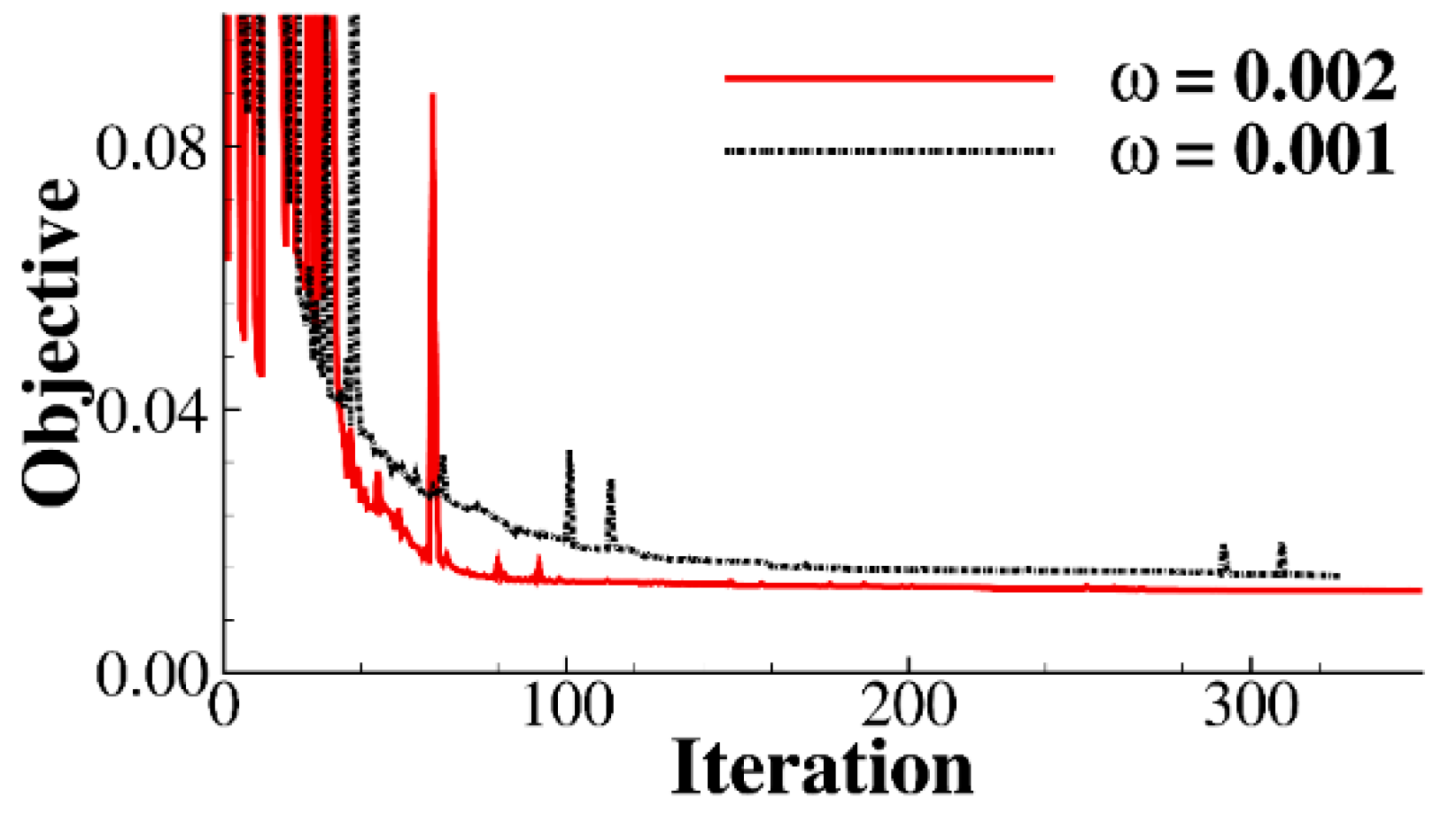
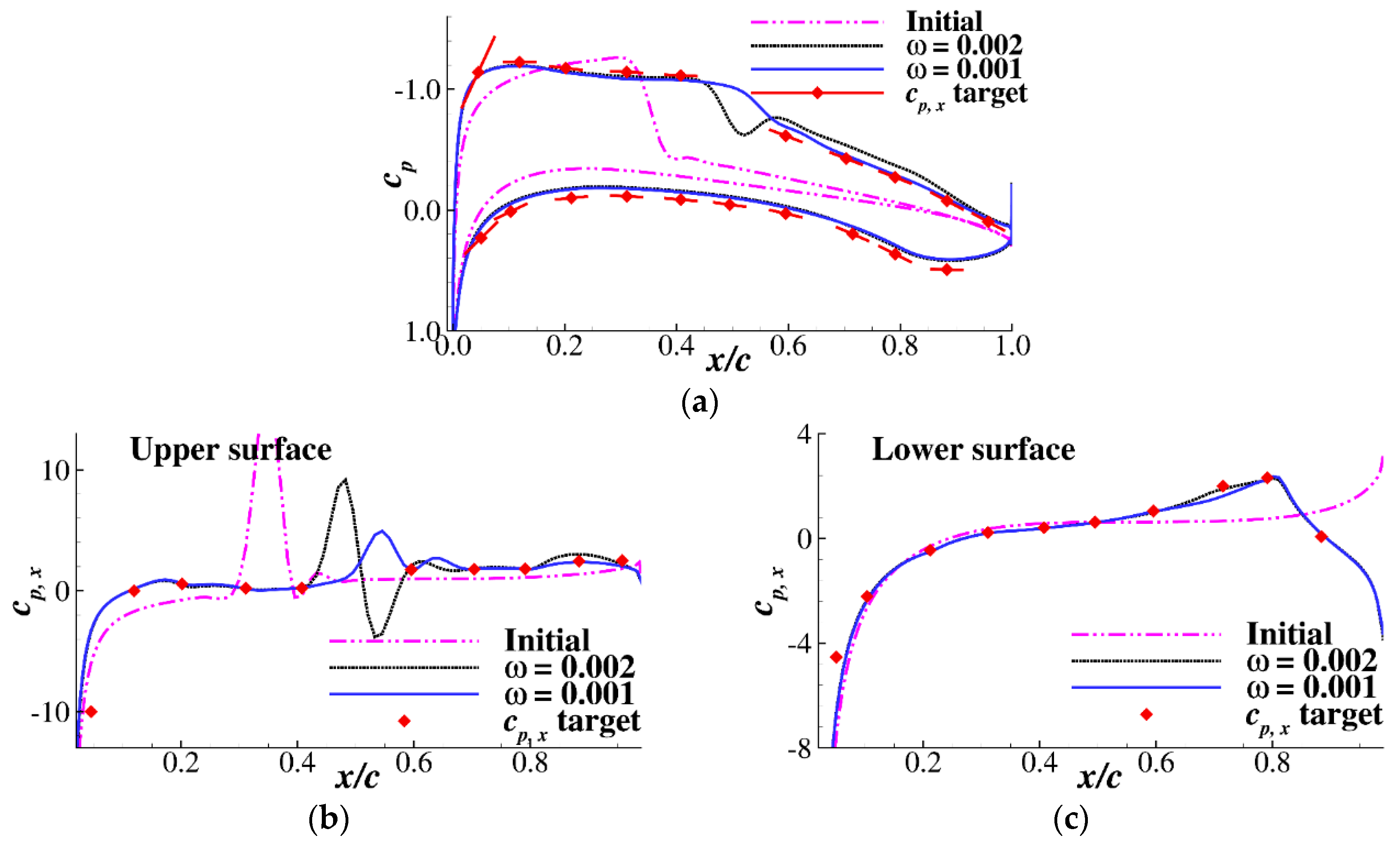
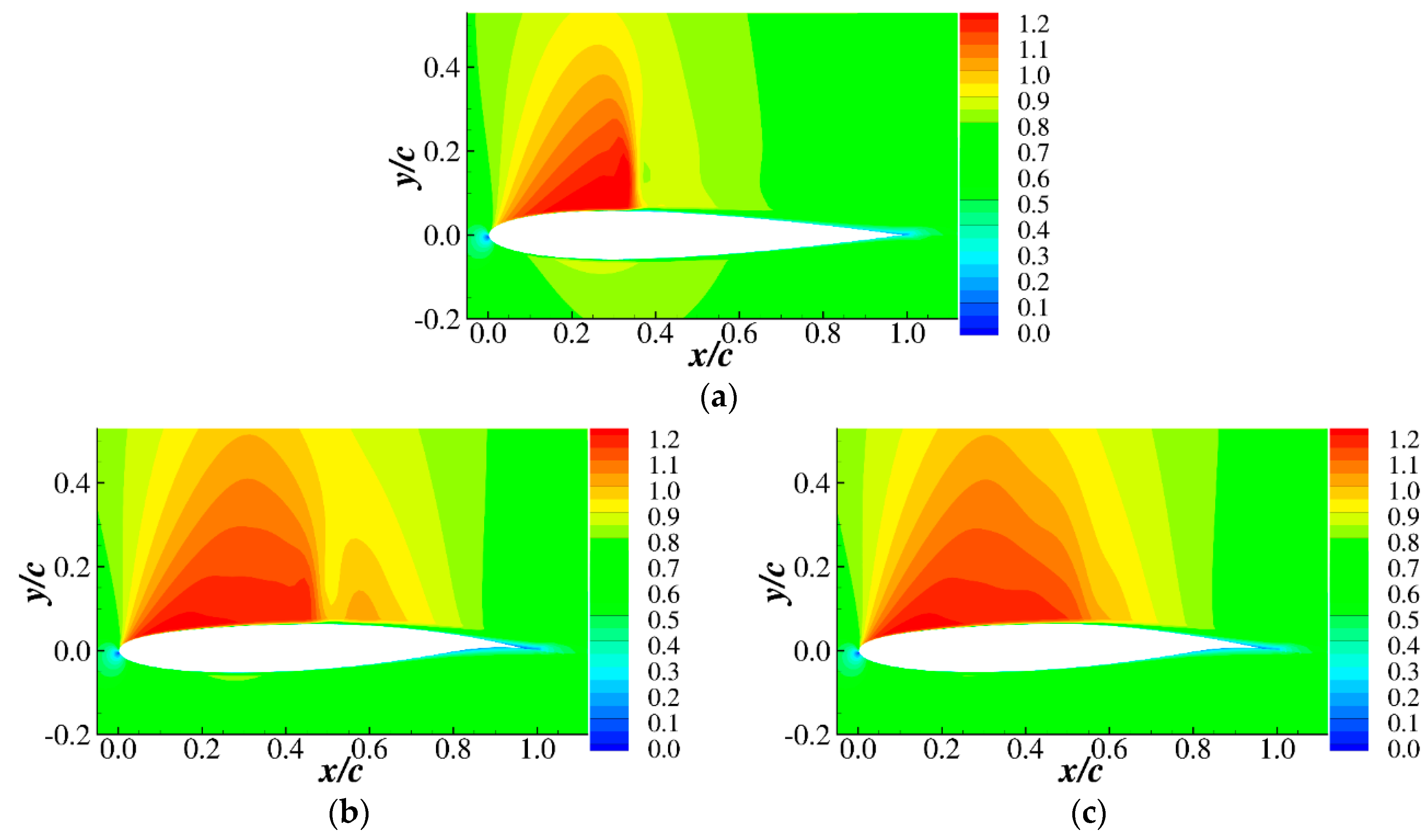
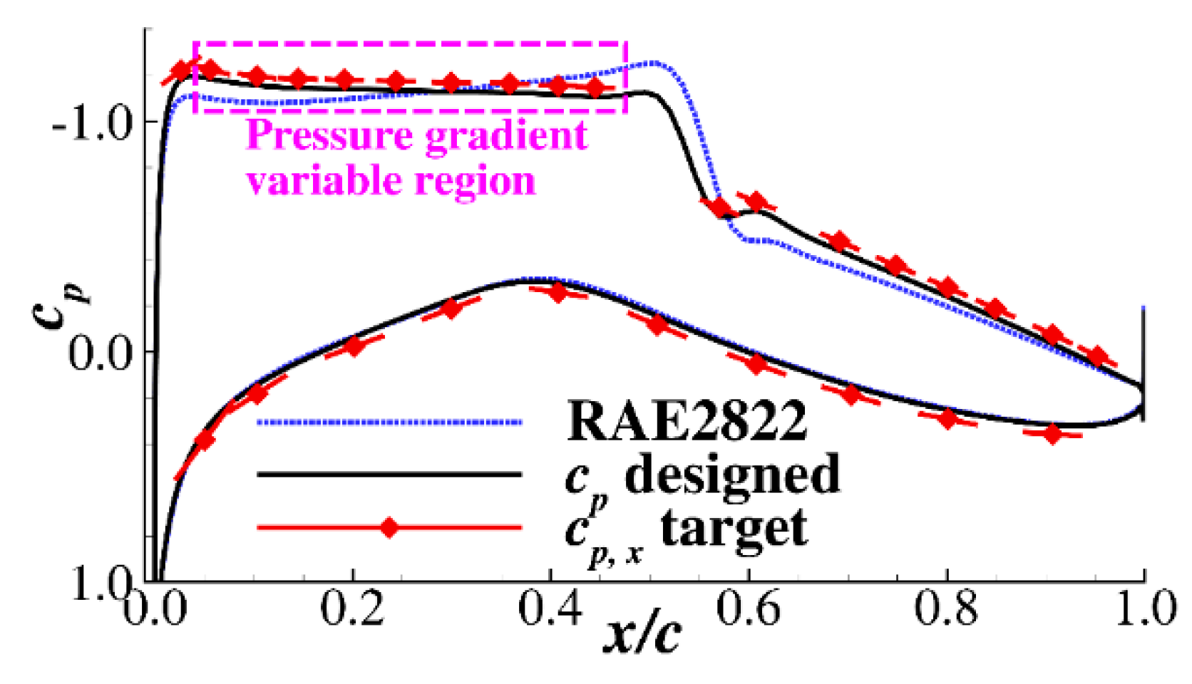
3.1. Supercritical Airfoil Design

A supercritical type pressure distribution was used as the design target for the first test case. A pressure distribution was manually drawn by the tool Javafoil [34], which is a well-known low-speed airfoil design tool. It does not have the ability to design a supercritical airfoil. However, it is a useful tool to sketch a typical supercritical type pressure distribution to represent the design expectation, as shown by the black dashed line in Figure 4.
If we directly used the pressure coefficient as the target for inverse design, we would not know whether the pressure distribution was feasible for a smooth airfoil; even if it was feasible, we could not make sure it had good aerodynamic performance. Consequently, the pressure gradients at twenty locations were used as the design target, as shown by the red diamonds in Figure 4, including ten points on the upper surface and ten points on the lower surface. These pressure gradients roughly characterize a supercritical type pressure distribution. The values of the pressure gradients, c p , x , at the twenty locations are also labeled in the figure. Positive values indicate an adverse pressure gradient, while negative values represent a favorable pressure gradient. The red segments in the figure indicate the slopes of the pressure with the labeled pressure gradient. The pressure gradient near the trailing edge was less than 3.0 to avoid flow separation. The pressure gradient on the front half of the upper surface had a weak adverse gradient to weaken the shockwave. The pressure gradient near x/c = 0.5 was not specified because we do not know which location was the best shockwave location for minimizing the drag coefficient. Consequently, the shockwave could be freely moved at 0.41 < x/c < 0.59 to obtain a minimum drag coefficient design.
It was obvious that the optimization was an ill-posed problem if the objective only had a pressure gradient because we could obtain countless solutions that satisfied the pressure gradient expectation. In the present computation, the lift and drag coefficients were also included in the inverse problem. This ensured that the candidate design not only satisfied the pressure gradient expectation but also optimized aerodynamic performance with a lift coefficient constraint. The flow conditions in this case were Ma = 0.73 and Re = 6.5 × 10⁶. The lift coefficient CL was constrained in the range of 0.80 ± 0.01, and the airfoil internal volume was no less than 0.064 to prevent the airfoil from becoming too thin. The thickness distribution was allowed to change slightly because the geometries of different types of airfoils are quite different. The thickness of the airfoil in the present study was not strictly constrained. The relative thickness at x/c = 0.40 of the airfoil was constrained to be no less than 0.98 times of the initial airfoil. The optimization problem of this case is defined as Equation (7). The cp,x,target is the target pressure distribution of the twenty prescribed locations. ω is a parameter that adjusts the weight between the drag coefficient and the target pressure gradient.
m i n   C D + ω i = 1 20 ( c p , x c p , x , target ) i 2 s . t .   C L = 0.80 ± 0.01 V o l u m e 0.064 t / c | x / c = 0.40 t / c | x / c = 0.40 , initial
A NACA0012 airfoil was used as the initial design. Two cases with ω = 0.001 and 0.002 were calculated for this case. The computation obtained different designs with different weights of the objective. Figure 5 shows the convergence histories of the two optimizations. More than 300 iterations were computed for both cases. The optimizations converge after 150 iterations. Two optimal airfoils were obtained from the computation.
Table 2 shows the aerodynamic coefficients of the airfoils. It is noteworthy that the angle of attack α was treated as a design variable, which is similar to the geometry variables. The derivatives of α were computed during the optimization. For a certain airfoil shape, the angle of attack was not changed to satisfy the design lift coefficient. The initial angle of attack was 2.0 degrees for the NACA0012 airfoil, so the initial lift coefficient was 0.359. The pressure gradient deviations i = 1 20 ( c p , x c p , x , target ) i 2 for both cases all converge to less than 2.0. The lift coefficients and volumes all fulfill the design constraints. The drag coefficients were greatly reduced, and the lift-to-drag ratios were increased considerably. Because the weights were different, the drag coefficients of the two optimized airfoils were slightly different.
Figure 6 shows the pressure and pressure gradient distributions of the initial and optimized airfoils. The target pressure gradient in Figure 6a is demonstrated by red segments with diamonds. It can be seen that both optimized airfoils have satisfactory pressure gradient tendencies compared with the design target. Figure 6b,c further presents the pressure gradient distributions of the upper and lower surfaces. It can be seen that the original airfoil had a quite different pressure gradient distribution. Because the leading edge had a large pressure gradient, the optimal designs and the target deviated slightly at the leading edge. In addition to the leading edge, the two optimized airfoils satisfied the target pressure gradient well. This demonstrates that the present inverse design method for the pressure gradient was effective.
In the present computation, the region at 0.41 < x/c < 0.59 on the upper surface had no design target because this region was where the shockwave is supposed to reside. The shockwave of a supercritical airfoil is very important for its transonic performance because the shockwave greatly influences the drag divergence characteristics. Aerodynamic designers usually need to design different airfoils or wings with different shockwave patterns and strengths to balance the trade-off between cruise efficiency and drag divergence performance [32].
Figure 7 shows the Mach number contours of the initial airfoil and the optimized airfoils. The initial airfoil had a strong shockwave and a large drag coefficient. The airfoil optimized with ω = 0.002 showed a weak shockwave at x/c = 0.50, and the drag coefficient was slightly higher than ω = 0.001 because the drag coefficient had a relatively lower weight in the optimization, while the ω = 0.001 case obtained a shockless airfoil, and its drag coefficient was the lowest. The present method was able to provide different airfoils with satisfactory pressure gradient patterns, while the shockwave characteristics were different for decision-making. The airfoil performance with different shockwaves is discussed in Section 4.

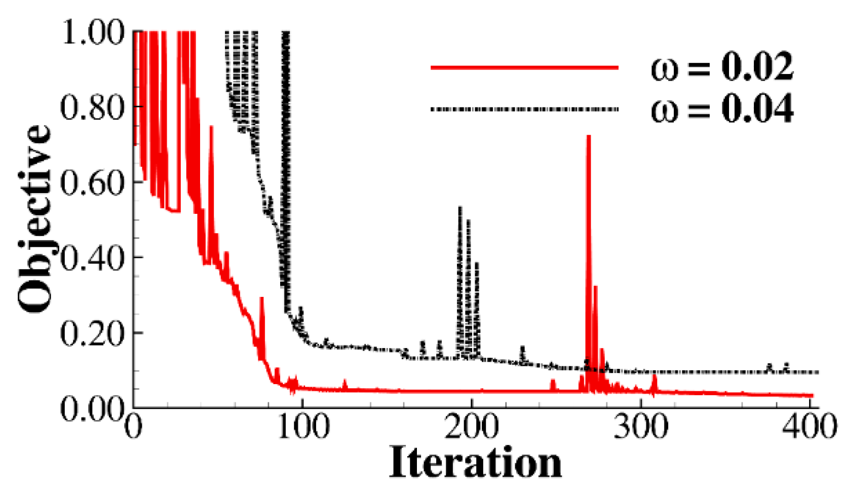
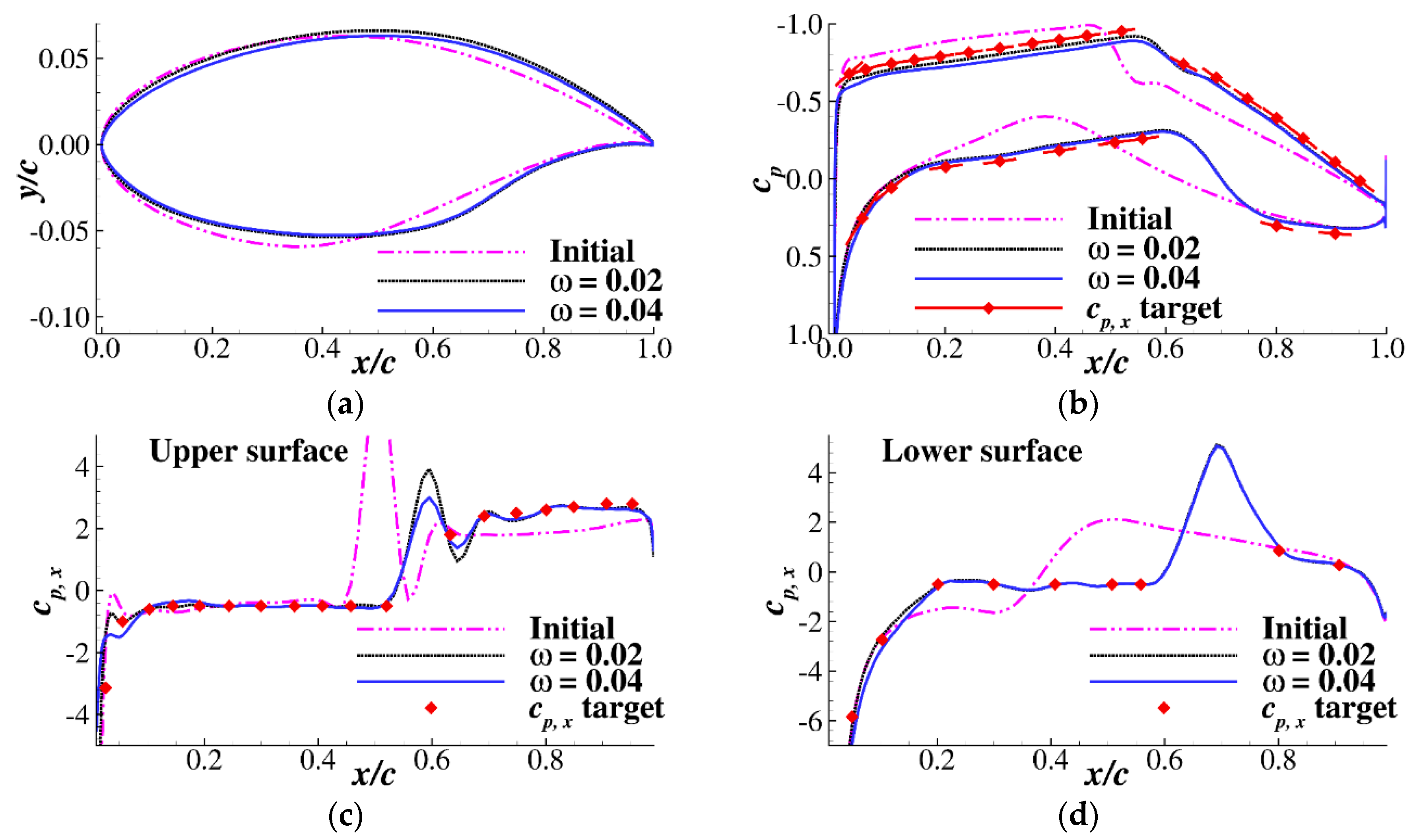
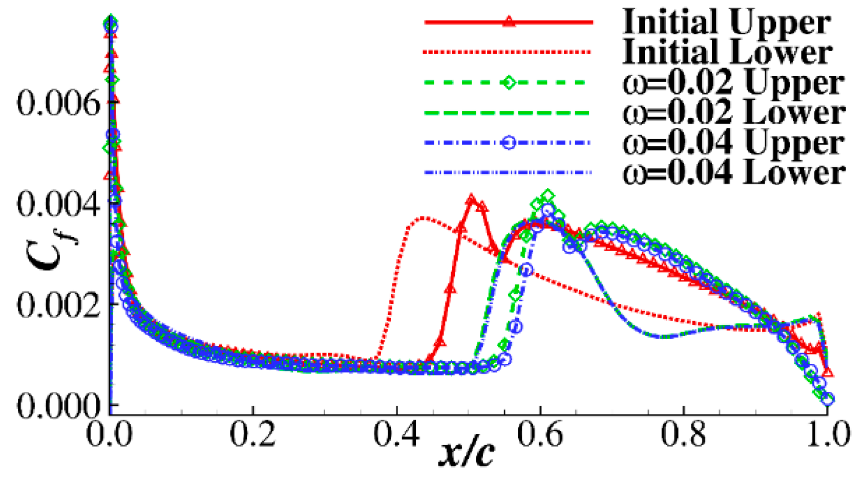
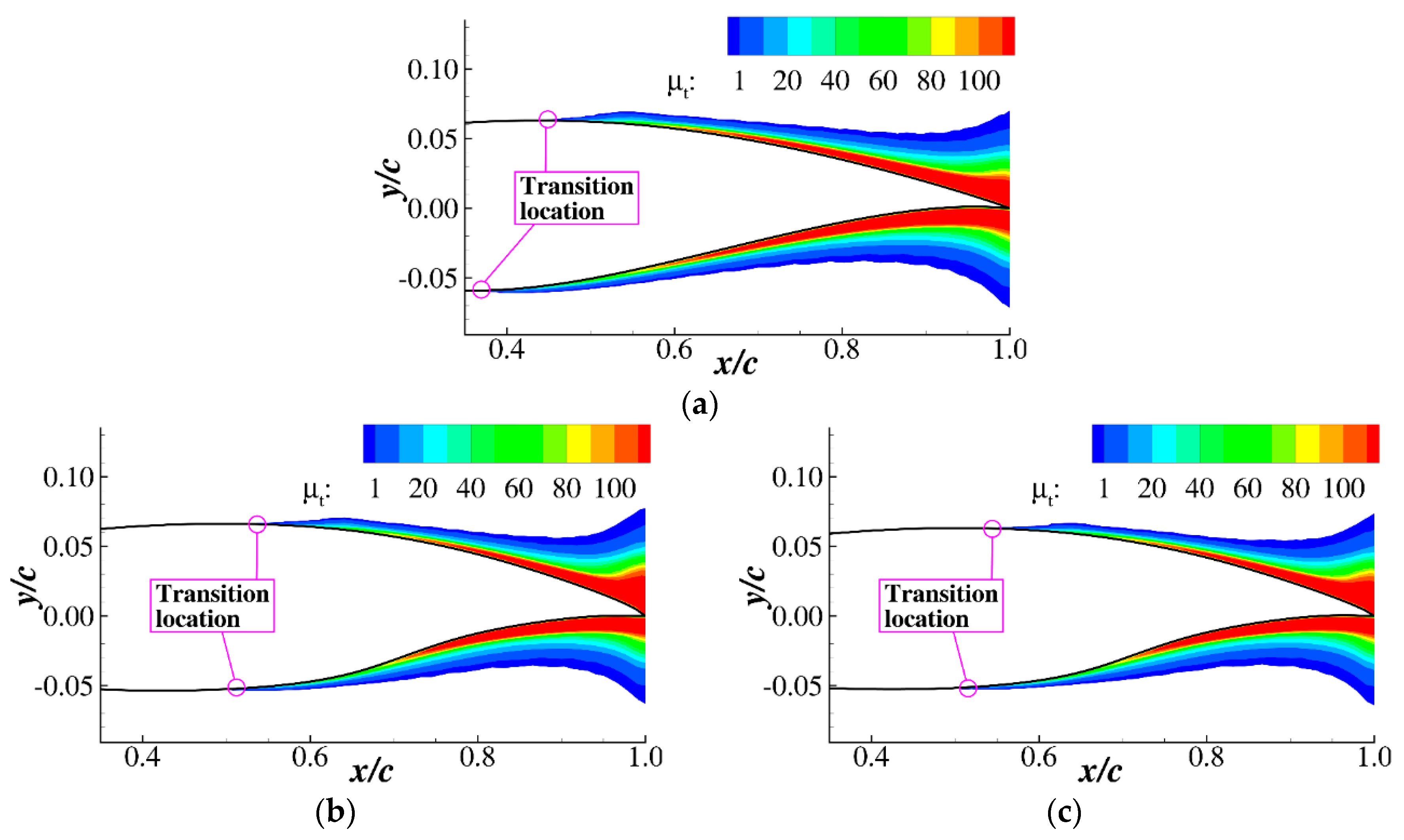
3.2. Supercritical Natural Laminar Flow Airfoil Design

In this subsection, a supercritical natural laminar flow airfoil (NLF) was optimized by the inverse method based on the pressure gradient target. Both the upper and lower surfaces of the airfoil had a favorable pressure gradient for suppressing the Tollmien–Schlichting wave and delaying the transition from laminar to turbulent flow [6].
The flow conditions were Ma = 0.73 and Re = 6.5 × 10⁶, and the lift coefficient was constrained in the range of 0.6 ± 0.005. The initial airfoil was the RAE2822 supercritical airfoil, and the initial AOA was 1.5 degrees. Because the pressure gradient at different locations had quite different values, the relative error of the actual pressure gradient cp,x and target pressure gradient cp,x,target was set as the design objective, as shown in Equation (8). The pressure gradients at 27 locations were set as the design targets, including 18 on the upper surface and 9 on the lower surface.
m i n   C D + ω i = 1 27 | c p , x c p , x , target 1.0 | i s . t .   C L = 0.06 ± 0.005 , V o l u m e 0.064
Two cases with different weights, ω = 0.02 and 0.04, were calculated. Figure 8 shows the histories of the optimizations. The objective descended very quickly in the first 100 iterations and then gradually converges. Two optimal designs were obtained through the optimization. The aerodynamic coefficients are shown in Table 3. It should be noted that the computation was carried out with the full turbulence SA model. Therefore, the drag coefficient was slightly increased to satisfy the pressure gradient requirement. The results of the transition computation are presented in the following.
Figure 9 shows the airfoil geometry, pressure, and pressure gradient distributions of the initial and optimized airfoils. It is clear in Figure 9a that the maximum thickness locations of the optimized airfoils were moved backward to obtain a favorable pressure gradient. The design expectation of the pressure gradient at the different locations is marked by the red segments with diamonds in Figure 9b. On the upper surface, the target pressure gradient was cp,x = −0.50 at 0.15 ≤ x/c ≤ 0.52, and the pressure gradient when x/c < 0.15 was even smaller than −0.50. The design target was changed from a favorable pressure gradient at x/c = 0.52 to an adverse pressure gradient at x/c = 0.63. The region of 0.52 < x/c < 0.63 was supposed to place the weak shockwave of the supercritical NLF airfoil. On the lower surface, the target pressure gradient was cp,x = −0.50 at 0.20 ≤ x/c ≤ 0.56 and was smaller than −0.50 when x/c < 0.20. The design target was changed from a favorable pressure gradient at x/c = 0.56 to an adverse pressure gradient at x/c = 0.80. The pressure recovery region of 0.56 ≤ x/c ≤ 0.80 was not constrained to explore more airfoil shapes. The pressure distributions of the two optimized airfoils were very similar. The airfoil optimized with ω = 0.02 had a slightly stronger shock wave and a higher drag coefficient. It can also be seen from Figure 9c,d that the target pressure gradients on both the upper and lower surfaces were achieved after the optimization, except there was minor deviation near the leading edge of the upper surface. Once again, the capability of the new inverse method was demonstrated to be effective by this supercritical NLF airfoil optimization case.
The airfoils were computed by the SST k-ω-γ-Reθ transition model [35] to validate the efficiency of the NLF design. The freestream turbulence intensity was 0.01%. The aerodynamic coefficients are listed in Table 4. It is clear that the drag coefficients were reduced by the transition computation. Figure 10 shows the friction coefficient distributions of the initial and optimized airfoils. The transition locations of the optimized airfoils were delayed by approximately 10–15% by the optimization of both the upper and lower surfaces. Figure 11 shows the eddy viscosity μ t / μ contours of the three airfoils. The eddy viscosity below 0.1 was blanked, and that of the y-coordinate was amplified. It can be seen that the location of the high eddy viscosity moved back. Consequently, the inverse design method with the favorable pressure gradient target had the capability of designing a supercritical natural laminar flow airfoil.

4. Influence of Pressure Gradient on Supercritical Airfoil Performance

In this section, supercritical airfoils with different upper surface pressure gradients were designed based on the inverse method. Then, the airfoils were numerically tested to study the drag creep and drag divergence behaviors.

4.1. Target Pressure Gradient of Supercritical Airfoil

The design targets of different supercritical airfoils were based on the pressure gradient distribution. The flow conditions were Ma = 0.73 and Re = 6.5 × 10⁶, and the lift coefficient CL was 0.8 ± 0.005. Pressure gradients at 28 points on the airfoil were used as the design target, including 18 points on the upper surface and 10 points on the lower surface. The RAE2822 airfoil was used as the initial design. The pressure gradient target was modified from the RAE2822 airfoil. As shown in Figure 12, the pressure gradient on the lower surface was the same as the RAE2822 airfoil, and the upper surface was adjusted. The pressure gradient at the front half of the upper surface was changed to an adverse pressure gradient or a very small favorable pressure gradient to suppress the shockwave strength. The adverse pressure gradient of the second half was also slightly strengthened to provide enough lift coefficient. The pressure gradient in the region 0.10 ≤ x/c ≤ 0.45 was adjustable in the optimization to design different airfoils. Optimizations with different pressure gradients were carried out. The design problem is defined as Equation (9). The weight is ω = 0.001.
m i n   C D + ω i = 1 28 | c p , x c p , x , target 1.0 | i s . t .   C L = 0.80 ± 0.005 , V o l u m e 0.064 , t / c | x / c = 0.40 t / c | x / c = 0.40 , initial

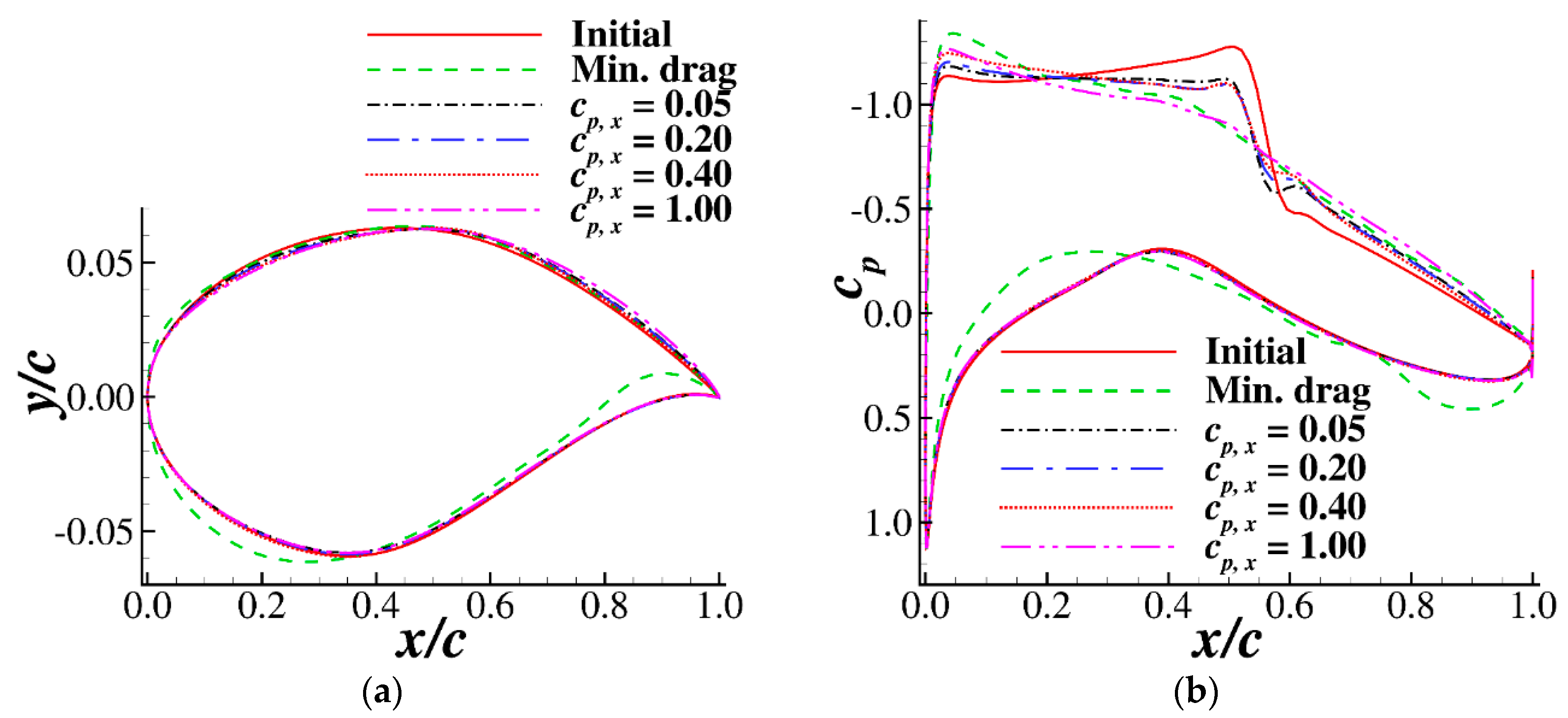
4.2. Characteristics of Airfoils with Different Upper Surface Pressure Gradients

Eight airfoils with different pressure gradients on the upper surface were designed by the method. Table 5 presents the aerodynamic coefficients of the airfoils. Two more airfoils are also listed in the table. One is the initial RAE2822 airfoil, and the other is an airfoil optimized by minimizing the drag coefficient without a pressure gradient target. The drag coefficient of the initial airfoil was the largest, and the airfoil optimized by minimizing the drag coefficient had the lowest drag. The drag coefficient monotonically decreased with increasing pressure gradient at 0.10 ≤ x/c ≤ 0.45.
Figure 13 shows the geometries and pressure distributions of the four airfoils designed with different pressure gradients, as well as the initial airfoil and the minimum drag airfoil. Because the target pressure gradients cp,x of the ten points on the lower surface were not modified, the shapes and pressure distributions of the lower surfaces of the inversely designed airfoils were almost the same as those of the RAE2822. However, the shape and pressure coefficient on the lower surface of the minimum drag airfoil were considerably changed with strong aft-loading emerging and front-loading disappearing. On the upper surface, the variations in the airfoil shapes were quite small, which confirms the highly nonlinear characteristics of the transonic flow. A small change in geometry may have had a strong effect on the shockwave and drag coefficient. The initial airfoil had a favorable pressure gradient on the upper surface before the shockwave, which increased the shock strength and deteriorated the drag coefficient. With the inverse design method, the expected pressure gradient can be easily achieved. The shockwave strength weakens with increasing adverse pressure gradient on the upper surface. The airfoil of the cp,x = 1.0 case was almost shockfree.
Figure 14 shows the pressure gradients on the upper surfaces of the airfoils of cp,x = 0.05 and 0.40. The front halves (x/c < 0.5) of the airfoils had different cp,x targets, and the designs satisfied the targets. The second halves (x/c > 0.5) had the same cp,x target. One can see that the pressure gradients near the shockwave location (0.5 < x/c < 0.6) had some deviations compared with that of the targets. However, the present inverse method was expressed as an optimization problem of the combination of the drag coefficient and pressure gradient target, which inherently includes a trade-off between the drag and the pressure distribution.

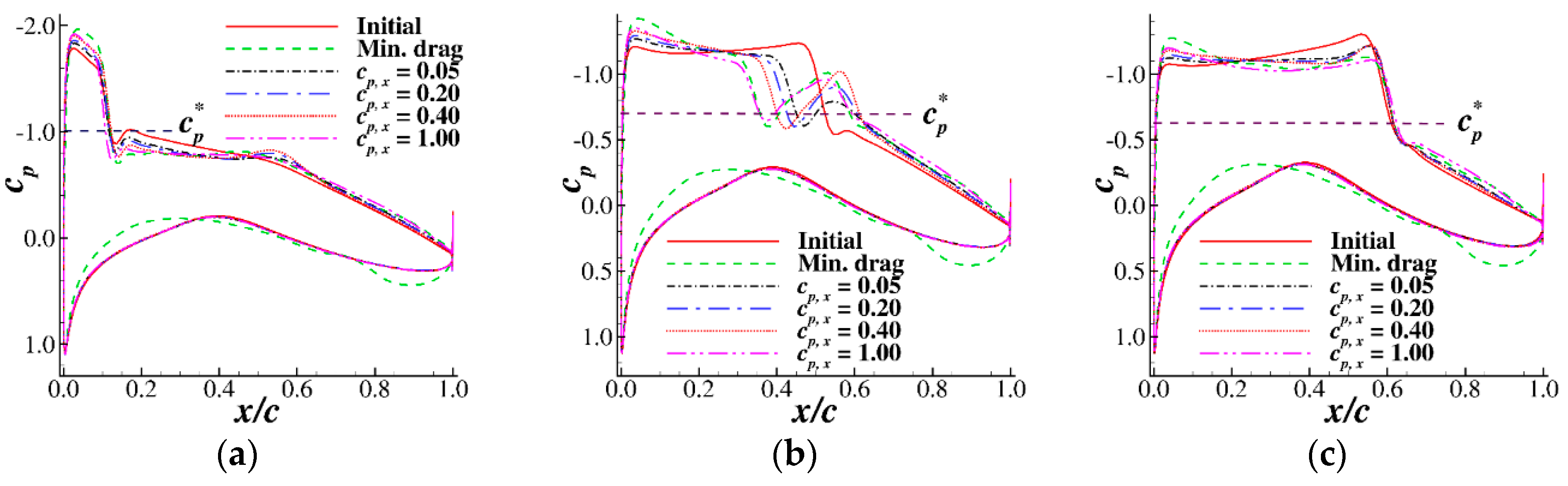
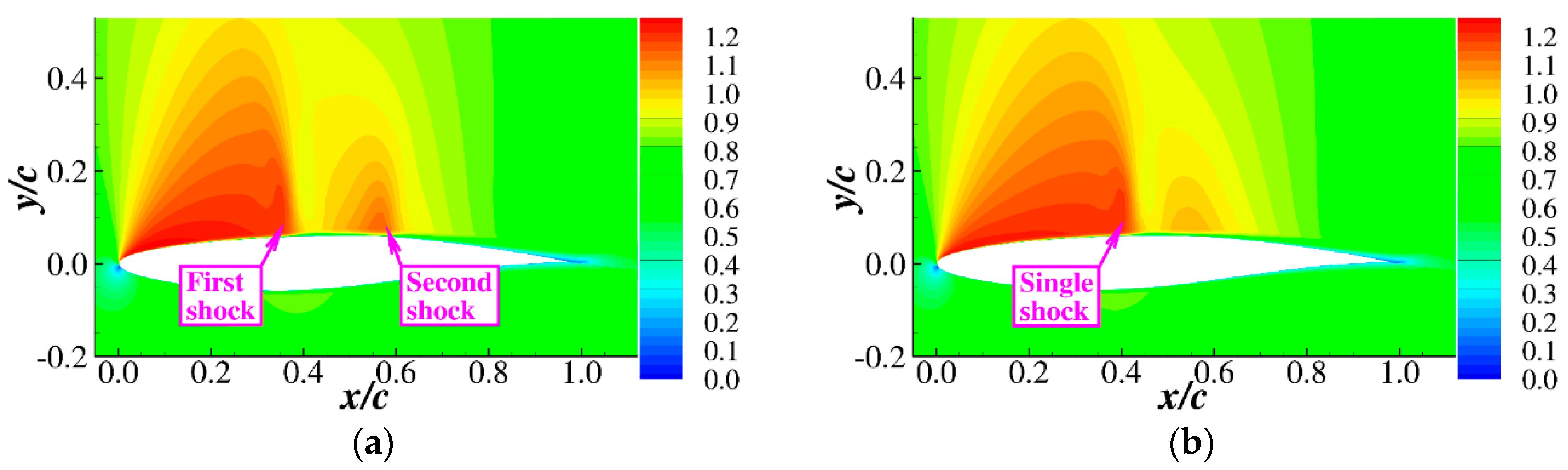
4.3. Drag Divergence Performance of Airfoils with Different Pressure Gradients

The upper surface pressure gradient had a strong effect on the shockwave strength, which is important for the drag creep and drag divergence characteristics of a supercritical airfoil. The drag creep phenomenon is where the drag slowly increases from the subcritical Mach number to the supercritical Mach number, and the drag divergence is the fast increase after the design Mach number [36]. Poor drag creep performance may decrease the efficiency of the second-segment climb phase of an aircraft and increase the thrust requirement of the engine. In contrast, the drag divergence performance influences the cruise efficiency of a civil aircraft when cruising at a higher speed or altitude. Both good drag creep performance and drag divergence performance are demanded for aircraft design.
Figure 15a shows the drag creep characteristics of the airfoils. The computations were carried out with the same lift coefficient CL = 0.800 and Reynolds number 6.5 × 10⁶. Under subcritical conditions, the drag coefficient slowly increased with increasing Mach number. The initial airfoil had the best drag creep performance, with the drag increasing the least from Ma = 0.45 to 0.65. In contrast, the minimum drag airfoil had the worst drag creep performance in that the drag increased dramatically. The second-segment climb phase of a civil aircraft is quite time consuming, especially for a short- or medium-range flight mission. Consequently, an airfoil optimized by minimizing the drag coefficient only may not be practical. Figure 16 further shows the pressure distributions of the airfoils. The critical pressure coefficient c p * is also marked in the figure, which is computed by Equation (10).
c p * = 2 γ M a 2 { [ 2 γ + 1 ( 1 + γ 1 2 M a 2 ) ] γ γ 1 1 }
Figure 15a is at Ma = 0.65. It is clear that the suction peak of the minimum drag airfoil was higher than those of the others, so the shock wave was stronger. At this Mach number, the drag coefficient monotonically increased with the suction peak. Moreover, for the airfoil inversely designed by the upper surface pressure gradient, the suction peak, and the drag coefficient at Ma = 0.65, also monotonically increased with the adverse pressure gradient.
Figure 15b shows the drag divergence characteristics of the airfoils. The initial airfoil had the worst drag divergence performance as the drag increased quickly when Ma > 0.72. The airfoil with the minimum drag had a “spoon” type drag curve because it had a high drag coefficient at a small Mach number and low drag at the design condition (Ma = 0.73). The curve of cp,x = 1.0 was similar to that of the minimum drag airfoil because this airfoil was similar to a shockfree airfoil, as shown in Figure 13b. The drag vs. Mach curves of cp,x = 0.05 and 0.2 were quite flat when Ma < 0.72, and they did not show obvious “spoon” type drag curves.
Figure 16b,c shows the pressure distributions of Ma = 0.72 and 0.74, which were slightly lower and higher than the design condition (Ma = 0.73). When Ma = 0.72, the initial airfoil presented a strong shockwave, while the other airfoils presented a reacceleration area after the first shock. Figure 17a shows the Mach number contour of the cp,x = 0.40 airfoil at Ma = 0.72. It is clear that the reacceleration area formed a second shock. The drag coefficient of the airfoil with double-shock compression was slightly lower than that with single-shock compression because the entropy production of a double shock was lower than that of a single shock when the pressure increase was the same [37]. However, the double shock made the drag curve not monotonically increase with the Mach number. Figure 17b also shows the flow field of cp,x = 0.05. The reacceleration area was quite weak, and no obvious double-shock phenomena appeared. When the Mach number was higher than the design Mach number of 0.73, the pressure distributions demonstrated strong shockwaves, as shown in Figure 17c. The drag coefficient was determined by the shockwave strength, i.e., the pressure difference before and after the shockwave.
Considering the lift-to-drag ratio at the design condition, the drag creep and the drag divergence characteristics, the airfoil optimized with cp,x = 0.20 had a stable performance under different Mach numbers and a moderate lift-to-drag ratio at the design condition. Consequently, the pressure gradient of cp,x = 0.20 on the front half of the upper surface was a satisfactory value for supercritical airfoil design. The airfoil of cp,x = 0.05 was also satisfactory with a stable performance; however, the lift-to-drag ratio was slightly lower than that of cp,x = 0.20.

5. Conclusions

This paper proposes an inverse design method based on the pressure gradient target. The adjoint method is adopted to compute the derivatives of the pressure gradient, and the sequential quadratic programming algorithm is used to find the optimal solution. The free form deformation method is applied for geometric deformation. The advantage of this method is that only a rough expectation of the pressure distribution pattern is required in the design process rather than a precise pressure coefficient under a certain lift coefficient and Mach number. The method will be further studied on a three-dimensional wing. The work of this paper can be summarized as:
(1) The computational method is validated well by the experimental data of the RAE2822 airfoil. Two test cases of inverse design, including a supercritical airfoil and a supercritical NLF airfoil, are used to test the effectiveness of the method. The results show that the method can design airfoils with good performance by target pressure gradients of less than 20 points on the upper surface and less than 10 points on the lower surface. The airfoil designed by the method has both low aerodynamic drag and an appropriate pressure distribution pattern. The supercritical natural laminar airfoil is also validated by the transition model and demonstrates good laminar performance.
(2) Several airfoils with different upper surface gradients are designed and compared. When the upper surface gradient before x/c = 0.5 is larger than 0.6, the airfoil tends to be shockfree. The drag creep and drag divergence characteristics of the airfoils are tested. The shockfree airfoil has deteriorated drag creep behavior, and the drag vs. Mach number curve becomes a spoon shape. The high leading edge suction peak is the reason for the poor drag creep performance. A double-shock phenomenon is observed on airfoils with large adverse pressure gradients. A pressure gradient cp,x = 0.2 for the front half of the upper surface is proposed for a supercritical airfoil to obtain both good drag creep and drag divergence performances.

Author Contributions

Conceptualization, Y.Z.; Data curation, Y.Z.; Formal analysis, H.C.; Investigation, C.Y.; Methodology, C.Y. and H.C. All authors have read and agreed to the published version of the manuscript.

Funding

This work was supported by the National Natural Science Foundation of China (91852108 and 11872230).

Acknowledgments

The authors would like to thank the Multidisciplinary Design Optimization Laboratory of the University of Michigan for providing the ADflow code under the GNU Lesser General Public License (LGPL).

Conflicts of Interest

The authors declare that they have no conflicts of interest with regard to this work.

References

  1. Zhang, Y.; Yin, Y. Study on Riblet Drag Reduction Considering the Effect of Sweep Angle. Energies 2019, 12, 3386. [Google Scholar] [CrossRef] [Green Version]
  2. Xu, Z.; Saleh, J.H.; Yang, V. Optimization of Supercritical Airfoil Design with Buffet Effect. AIAA J. 2019, 57, 4343–4353. [Google Scholar] [CrossRef]
  3. Driver, J.; Zingg, D.W. Optimized Natural-Laminar-Flow Airfoils. In Proceedings of the 44th AIAA Aerospace Sciences Meeting and Exhibit, Reno, NV, USA, 9–12 January 2006. [Google Scholar]
  4. Raheem, M.A.; Edi, P.; Pasha, A.A.; Rahman, M.M.; Juhany, K.A. Numerical Study of Variable Camber Continuous Trailing Edge Flap at Off-Design Conditions. Energies 2019, 12, 3185. [Google Scholar] [CrossRef] [Green Version]
  5. Zhao, T.; Zhang, Y.; Chen, H.; Chen, Y.; Zhang, M. Supercritical Wing Design Based on Airfoil Optimization and 2.75D Transformation. Aerosp. Sci. Technol. 2016, 56, 168–182. [Google Scholar] [CrossRef]
  6. Zhang, Y.; Fang, X.; Chen, H.; Fu, S.; Duan, Z.; Zhang, Y. Supercritical Natural Laminar Flow Airfoil Optimization for Regional Aircraft Wing Design. Aerosp. Sci. Technol. 2015, 43, 152–164. [Google Scholar] [CrossRef]
  7. Edi, P.; Fielding, J.P. Civil-Transport Wing Design Concept Exploiting New Technologies. J. Aircr. 2006, 43, 932–940. [Google Scholar] [CrossRef]
  8. Gopalarathnam, A.; Selig, M.S. Hybrid Inverse Airfoil Design Method for Complex Three-Dimensional Lifting Surfaces. J. Aircr. 2002, 39, 409–417. [Google Scholar] [CrossRef] [Green Version]
  9. Selig, M.S.; Maughmert, M.D. Multipoint Inverse Airfoil Design Method Based on Conformal Mapping. AIAA J. 1992, 30, 1162–1170. [Google Scholar] [CrossRef]
  10. Malone, J.B.; Narramoret, J.C.; Sankar, L.N. Airfoil Design Method Using the Navier-Stokes Equations. J. Aircr. 1991, 28, 216–224. [Google Scholar] [CrossRef]
  11. Dadone, A.; Grossman, B. Fast Convergence of Viscous Airfoil Design Problems. AIAA J. 2002, 40, 1997–2005. [Google Scholar] [CrossRef]
  12. Gopalarathnam, A.; Selig, M.S. Low-Speed Natural-Laminar-Flow Airfoils: Case Study in Inverse Airfoil Design. J. Aircr. 2001, 38, 57–63. [Google Scholar] [CrossRef] [Green Version]
  13. Eyi, S.; Lee, K.D. Inverse Airfoil Design Using the Navier-Stokes Equations. In Proceedings of the 7th Applied Aerodynamics Conference, Irvine, CA, USA, 16–19 February 1993. [Google Scholar]
  14. Gardner, B.A.; Selig, M.S. Airfoil Design Using a Genetic Algorithm and an Inverse Method. In Proceedings of the 41st Aerospace Sciences Meeting and Exhibit, Reno, NV, USA, 6–9 January 2003. [Google Scholar]
  15. Hacioglu, A. Fast Evolutionary Algorithm for Airfoil Design via Neural Network. AIAA J. 2007, 45, 2196–2203. [Google Scholar] [CrossRef]
  16. Bui-Thanh, T.; Damodaran, M.; Willcox, K. Aerodynamic Data Reconstruction and Inverse Design Using Proper Orthogonal Decomposition. AIAA J. 2004, 42, 1505–1516. [Google Scholar] [CrossRef] [Green Version]
  17. Ylmaz, E.; German, B.J. A Deep Learning Approach to an Airfoil Inverse Design Problem. In Proceedings of the 2018 Multidisciplinary Analysis and Optimization Conference, Atlanta, GA, USA, 25–29 June 2018. [Google Scholar]
  18. Sekar, V.; Zhang, M.; Shu, C.; Khoo, B.C. Inverse Design of Airfoil Using a Deep Convolutional Neural Network. AIAA J. 2019, 57, 993–1003. [Google Scholar] [CrossRef]
  19. Tang, H.; Lei, Y.; Li, X.; Gao, K.; Li, Y. Aerodynamic Shape Optimization of a Wavy Airfoil for Ultra-Low Reynolds Number Regime in Gliding Flight. Energies 2020, 13, 467. [Google Scholar] [CrossRef] [Green Version]
  20. Jameson, A. Aerodynamic Design via Control Theory. J. Sci. Comput. 1988, 3, 233–260. [Google Scholar] [CrossRef] [Green Version]
  21. Mader, C.A.; Martins, J.R.R.A.; Alonso, J.J.; Weide, E. ADjoint: An Approach for the Rapid Development of Discrete Adjoint Solvers. AIAA J. 2008, 46, 863–873. [Google Scholar] [CrossRef]
  22. He, P.; Mader, C.A.; Martins, J.R.R.; Maki, J. DAFoam: An Open-Source Adjoint Framework for Multidisciplinary Design Optimization with OpenFOAM. AIAA J. 2019, 58, 1304–1319. [Google Scholar] [CrossRef]
  23. Li, R.; Deng, K.; Zhang, Y.; Chen, H. Pressure Distribution Guided Supercritical Wing Optimization. Aeronaut. J. 2018, 31, 1842–1854. [Google Scholar] [CrossRef]
  24. Kenway, G.K.W.; Mader, C.A.; He, P.; Martins, J.R.R.A. Effective Adjoint Approaches for Computational Fuid Dynamics. Prog. Aerosp. Sci. 2019, 110, 100542. [Google Scholar] [CrossRef]
  25. Jameson, A.; Schmidt, W.; Turkel, E. Numerical Solution of the Euler Equations by Finite Volume Methods Using Runge–Kutta Time Stepping Schemes. In Proceedings of the 14th Fluid and Plasma Dynamics Conference, Palo Alto, CA, USA, 13–25 June 1981. [Google Scholar]
  26. Spalart, P.; Allmaras, S. A One-Equation Turbulence Model for Aerodynamic Flows. In Proceedings of the 30th Aerospace Sciences Meeting and Exhibit, Reno, NV, USA, 6–9 January 1992. [Google Scholar]
  27. Cook, P.H.; McDonald, M.A.; Firmin, M.C.P. Experimental Data Base for Computer Program Assessment; Aerofoil RAE 2822—Pressure Distributions, and Boundary Layer and Wake Measurements; AGARD Advisory Report No. 138; Advisory Group for Aerospace Research and Development: Neuilly sur Seine, France, 1979. [Google Scholar]
  28. Hascoet, L.; Pascual, V. The Tapenade Automatic Differentiation Tool: Principles, Model, and Specification. ACM Trans. Math. Softw. 2012, 7957. [Google Scholar] [CrossRef] [Green Version]
  29. Gill, P.E.; Murray, W.; Saunders, M.A. SNOPT: An SQP Algorithm for Large-Scale Constrained Optimization. Siam. Rev. 2005, 47, 99–131. [Google Scholar] [CrossRef]
  30. Zhang, T.; Wang, Z.; Huang, W.; Yan, L. A Review of Parametric Approaches Specific to Aerodynamic Design Process. Acta. Astronaut. 2018, 145, 319–331. [Google Scholar] [CrossRef]
  31. Zhao, K.; Gao, Z.; Huang, J.; Li, Q. Aerodynamic Optimization of Rotor Airfoil Based on Multi-Layer Hierarchical Constraint Method. Chin. J. Aeronaut. 2016, 29, 1541–1552. [Google Scholar] [CrossRef] [Green Version]
  32. Li, J.; Gao, Z.; Huang, J.; Zhao, K. Robust Design of NLF Airfoils. Chin. J. Aeronaut. 2013, 26, 309–318. [Google Scholar] [CrossRef] [Green Version]
  33. Han, Z.H.; Chen, J.; Zhang, K.S.; Xu, Z.M.; Zhu, Z.; Song, W.P. Aerodynamic Shape Optimization of Natural-Laminar-Flow Wing Using Surrogate-Based Approach. AIAA J. 2018, 56, 2579–2593. [Google Scholar] [CrossRef]
  34. Hepperle, M. JavaFoil—Analysis of Airfoils. Available online: http://www.mh-aerotools.de/airfoils/javafoil.htm (accessed on 2 July 2020).
  35. Menter, F.R.; Langtry, R.B.; Likki, S.R.; Suzen, Y.B.; Huang, P.G.; Völker, S. A Correlation-Based Transition Model Using Local Variables-Part I: Model Formulation. J. Turbomach. 2006, 128, 413–422. [Google Scholar] [CrossRef]
  36. Harris, C.D. NASA Supercritical Airfoils: A Matrix of Family-Related Airfoils; NASA-TP-2969; NASA Langley Research Center: Hampton, VA, USA, 1990.
  37. Liepmann, H.W.; Roshko, A. Elements of gasdynamics. In Waves in Supersonic Flow; Dover Publications: New York, NY, USA, 2001; Chapter 4; pp. 84–123. [Google Scholar]
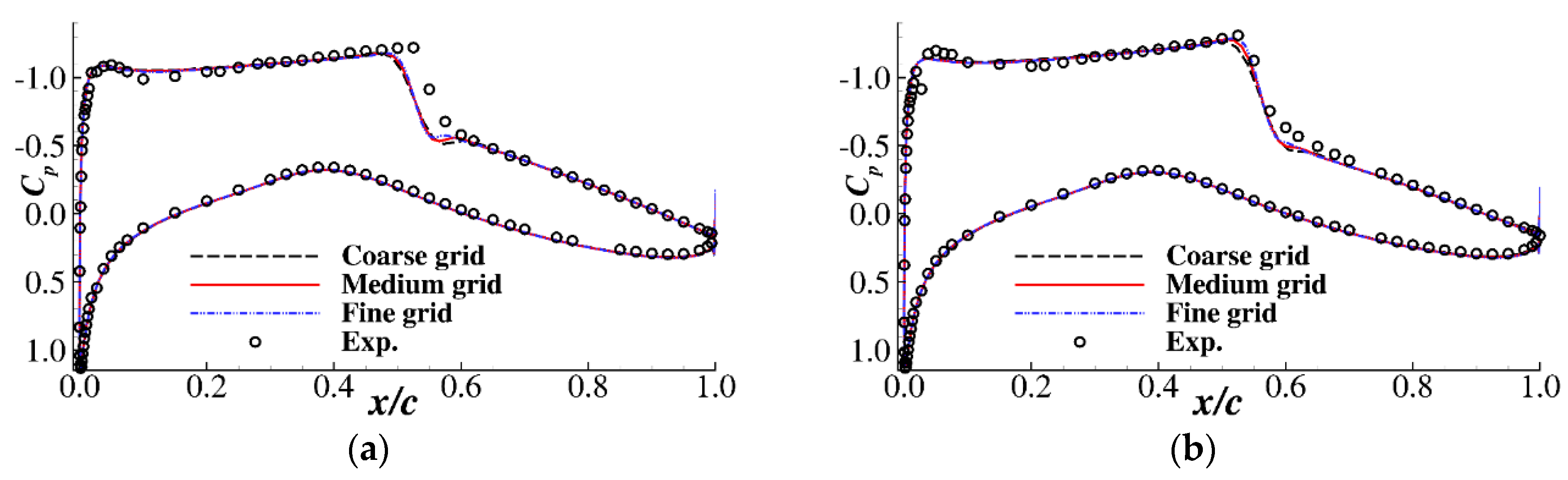
Figure 1. Computational grid of the RAE2822 airfoil (257 × 129 points).
Energies 13 03400 g001
Figure 2. Pressure coefficient comparisons for the RAE2822 airfoil. (a) Case 6: Ma = 0.725, Re = 6.5 × 10⁶, CL = 0.743; (b) Case 9: Ma = 0.730, Re = 6.5 × 10⁶, CL = 0.803.
Energies 13 03400 g002
Figure 3. Free-form deformation (FFD) frame of the airfoil optimization.
Energies 13 03400 g003
Figure 4. Pressure gradient target of a supercritical type airfoil.
Energies 13 03400 g004
Figure 5. Convergence histories of the optimizations with different weights.
Energies 13 03400 g005
Figure 6. Pressure and pressure gradient distributions of the airfoils. (a) Pressure distribution; (b) pressure gradient of the upper surface; and (c) pressure gradient of the lower surface.
Energies 13 03400 g006
Figure 7. Mach number contours of the initial airfoil and the optimized airfoils. (a) Initial airfoil; (b) optimized airfoil with ω = 0.002; and (c) optimized airfoil with ω = 0.001.
Energies 13 03400 g007
Figure 8. Optimization histories of the supercritical natural laminar flow (NLF) airfoil.
Energies 13 03400 g008
Figure 9. Airfoil, pressure and pressure gradient distributions of the supercritical NLF airfoil optimization. (a) Airfoil geometry; (b) pressure distribution; (c) pressure gradient of the upper surface; and (d) Pressure gradient of the lower surface.
Energies 13 03400 g009
Figure 10. Friction coefficients of the initial and optimized airfoils.
Energies 13 03400 g010
Figure 11. Eddy viscosity contours of the airfoils. (a) Initial airfoil; (b) optimized with ω = 0.02; and (c) optimized with ω = 0.04.
Energies 13 03400 g011
Figure 12. Pressure gradient target of supercritical airfoil.
Energies 13 03400 g012
Figure 13. Geometries and pressure distributions of the airfoils (Ma = 0.73, Re = 6.5 × 10⁶, CL = 0.800). (a) Airfoil geometries; (b) pressure distributions.
Energies 13 03400 g013
Figure 14. Pressure gradients on the upper surfaces of two airfoils (Ma = 0.73, Re = 6.5 × 10⁶, CL = 0.800).
Energies 13 03400 g014
Figure 15. Drag creep and drag divergence of the airfoils (Re = 6.5 × 10⁶, CL = 0.800). (a) Drag creep; (b) drag divergence.
Energies 13 03400 g015
Figure 16. Pressure distributions at different Mach numbers (Re = 6.5 × 10⁶, CL = 0.800). (a) Ma = 0.65; (b) Ma = 0.72; and (c) Ma = 0.74.
Energies 13 03400 g016
Figure 17. Flow fields of airfoils at Ma = 0.72, Re = 6.5 × 10⁶, CL = 0.800. (a) cp,x = 0.40; (b) cp,x = 0.05.
Energies 13 03400 g017
Table 1. Force coefficient comparisons of the RAE2822 airfoil.
CaseConfigurationα (°)Lift Coefficient CLDrag Coefficient CD
Case 6Experiment [27]2.920.7430.0127
Coarse grid2.340.7430.01245
Medium grid2.310.7430.01219
Fine grid2.290.7430.01215
Case 9Experiment [27]3.190.8030.0168
Coarse grid2.660.8030.01679
Medium grid2.600.8030.01628
Fine grid2.570.8030.01613
Table 5. Aerodynamic performance of the airfoils with different pressure gradients (Ma = 0.73, Re = 6.5 × 10⁶).
No.Target cp,x at 0.10 ≤ x/c ≤ 0.45AlphaLift CoefficientDrag CoefficientLift-To-Drag Ratio
Initial---2.610.8000.0161849.44
1-0.052.330.8000.0124264.41
20.052.400.8000.0122765.20
30.12.440.8000.0121765.74
40.22.400.8000.0115769.14
50.42.430.8000.0111671.68
60.62.420.8000.0112171.36
70.82.360.8000.0111172.01
81.02.310.8000.0110772.27
9Without cp,x target1.750.8000.0107774.28
Table 2. Aerodynamic coefficients of the airfoils (Ma = 0.73, Re = 6.5 × 10⁶).
Initial AirfoilOptimized with ω = 0.001Optimized with ω = 0.002
Angle of attack α2.001.691.61
Lift coefficient CL0.3590.7910.792
Drag coefficient CD0.013180.010890.01165
Lift-to-drag ratio27.2472.6367.98
Pressure gradient deviation i = 1 20 ( c p , x c p , x , target ) i 2 49.961.661.57
Airfoil volume0.06740.06420.0654
Table 3. Aerodynamic performance of the airfoils (Ma = 0.73, Re = 6.5 × 10⁶).
Original AirfoilOptimized with ω = 0.02Optimized with ω = 0.04
Angle of attack α1.501.391.46
Lift coefficient CL0.5920.6010.595
Drag coefficient CD (Full turbulent)0.010040.010840.01047
Lift-to-drag ratio (Full turbulent)58.9655.4456.83
Pressure gradient deviation i = 1 27 | c p , x / c p , x , target 1.0 | i 37.421.122.10
Airfoil volume0.06490.06810.0650
Table 4. Transition computations of the airfoils (Ma = 0.73, Re = 6.5 × 10⁶).
Original AirfoilOptimized with ω = 0.02Optimized with ω = 0.04
Angle of attack α1.170.991.05
Lift coefficient CL0.6000.6000.600
Drag coefficient CD0.006240.006090.00599

