Optimized Adaptive Overcurrent Protection Using Hybridized Nature-Inspired Algorithm and Clustering in Microgrids


Abstract
1. Introduction
1.1. Microgrid Protection Challenges
1.2. Literature Review
1.3. Methodology and Paper Structure
2. Adaptive Protection with Relay Coordination
2.1. Overcurrent Protection
2.2. Adaptive Overcurrent Protection
Clustering of Topologies
2.3. Protection Coordination with Optimization
2.3.1. Different Objective Functions
2.3.2. Optimization Algorithms and Constraint Handling
3. Problem Formulation and Simulation
3.1. Modified IEEE 14-Bus System
Single Element Contingencies
3.2. Load Flow and Short Circuit Analysis
3.3. Optimization Algorithm Implementation
3.3.1. Objective Function Formulation
3.3.2. Constraint Formulation
3.4. WCMFO Algorithm
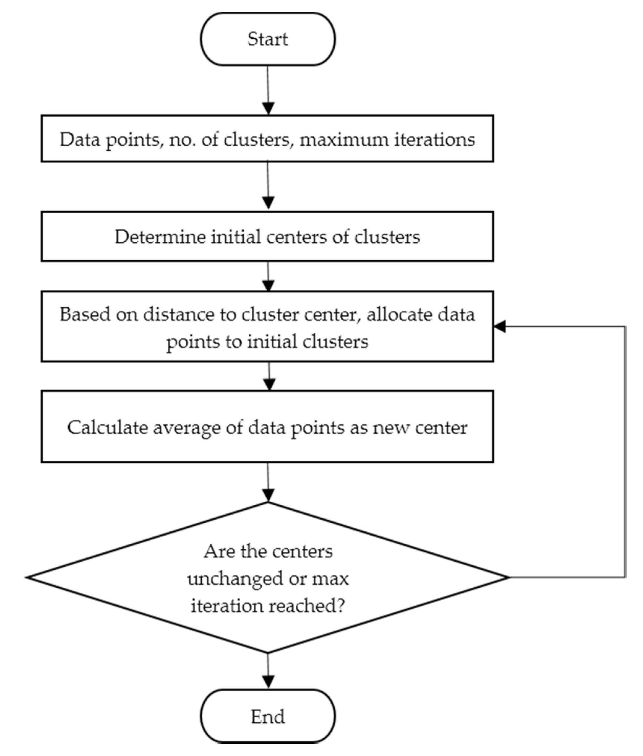
3.5. Clustering for Adaptive Protection
4. Results and Discussion
5. Conclusions
Author Contributions
Funding
Acknowledgments
Conflicts of Interest
References
- Tanrioven, M. Reliability and cost–benefits of adding alternate power sources to an independent micro-grid community. J. Power Sources 2005, 150, 136–149. [Google Scholar] [CrossRef]
- Senarathna, T.S.S.; Udayanga Hemapala, K.T.M. Department of Electrical Engineering, University of Moratuwa, Moratuwa, Sri Lanka Review of adaptive protection methods for microgrids. AIMS Energy 2019, 7, 557–578. [Google Scholar] [CrossRef]
- Maqbool, U.; Khan, U.A. Fault current analysis for grid-connected and Islanded Microgrid modes. In Proceedings of the 2017 13th International Conference on Emerging Technologies (ICET), Islamabad, Pakistan, 27–28 December 2017; IEEE: Piscataway, NJ, USA, 2018; pp. 1–5. [Google Scholar]
- Shah, R.; Goli, P.; Shireen, W. Adaptive Protection Scheme for a Microgrid with High Levels of Renewable Energy Generation. In Proceedings of the 2018 Clemson University Power Systems Conference (PSC), Charleston, SC, USA, 4–7 September 2018; IEEE: Piscataway, NJ, USA, 2019; pp. 1–7. [Google Scholar]
- Gomes, M.; Coelho, P.; Moreira, C. Microgrid protection schemes. In Microgrids Design and Implementation; Zambroni de Souza, A.C., Castilla, M., Eds.; Springer International Publishing: Cham, Switzerland, 2019; pp. 311–336. ISBN 978-3-319-98686-9. [Google Scholar]
- Lotfi-fard, S.; Faiz, J.; Iravani, R. Improved overcurrent protection using symmetrical components. IEEE Trans. Power Deliv. 2007, 22, 843–850. [Google Scholar] [CrossRef]
- Wang, X.; Li, Y.; Yu, Y. Research on the relay protection system for a small laboratory-scale microgrid system. In Proceedings of the 2011 6th IEEE Conference on Industrial Electronics and Applications, Beijing, China, 21–23 June 2011; IEEE: Piscataway, NJ, USA, 2011; pp. 2712–2716. [Google Scholar]
- Rockefeller, G.D.; Wagner, C.L.; Linders, J.R.; Hicks, K.L.; Rizy, D.T. Adaptive transmission relaying concepts for improved performance. IEEE Trans. Power Deliv. 1988, 3, 1446–1458. [Google Scholar] [CrossRef]
- Prasai, A.; Du, Y.; Paquette, A.; Buck, E.; Harley, R.; Divan, D. Protection of meshed microgrids with communication overlay. In Proceedings of the 2010 IEEE Energy Conversion Congress and Exposition, Atlanta, GA, USA, 12–16 September 2010; IEEE: Piscataway, NJ, USA, 2011; pp. 64–71. [Google Scholar]
- International Electrotechnical Commission. Communication Networks and Systems for Power Utility Automation—Part 3: General Requirements. (IEC 61850-3:2013). 2013. Available online: https://webstore.iec.ch/publication/6010 (accessed on 15 May 2020).
- Ustun, T.S.; Ozansoy, C.; Zayegh, A. Modeling of a centralized microgrid protection system and distributed energy resources according to IEC 61850-7-420. IEEE Trans. Power Syst. 2012, 27, 1560–1567. [Google Scholar] [CrossRef]
- Ustun, T.S.; Ozansoy, C.; Zayegh, A. A microgrid protection system with central protection unit and extensive communication. In Proceedings of the 2011 10th International Conference on Environment and Electrical Engineering, Rome, Italy, 8–11 May 2011; IEEE: Piscataway, NJ, USA, 2011; pp. 1–4. [Google Scholar]
- Chaitanya, B.K.; Soni, A.K.; Yadav, A. Communication assisted fuzzy based adaptive protective relaying scheme for Microgrid. J. Power Technol. 2018, 98, 57–69. [Google Scholar]
- Lin, H.; Guerrero, J.M.; Jia, C.; Tan, Z.-H.; Vasquez, J.C.; Liu, C. Adaptive overcurrent protection for microgrids in extensive distribution systems. In Proceedings of the IECON 2016—42nd Annual Conference of the IEEE Industrial Electronics Society, Florence, Italy, 23–26 October 2016; IEEE: Piscataway, NJ, USA, 2016; pp. 4042–4047. [Google Scholar]
- Bapeswara Rao, V.V.; Sankara Rao, K. Computer aided coordination of directional relays: Determination of break points. IEEE Trans. Power Deliv. 1988, 3, 545–548. [Google Scholar] [CrossRef]
- Jenkins, L.; Khincha, H.P.; Shivakumar, S.; Dash, P.K. An application of functional dependencies to the topological analysis of protection schemes. IEEE Trans. Power Deliv. 1992, 7, 77–83. [Google Scholar] [CrossRef]
- Zhu, X. Computational intelligence techniques and applications. In Computational Intelligence Techniques in Earth and Environmental Sciences; Islam, T., Srivastava, P.K., Gupta, M., Zhu, X., Mukherjee, S., Eds.; Springer: Dordrecht, The Netherlands, 2014; pp. 3–26. ISBN 978-94-017-8641-6. [Google Scholar]
- Yang, X.-S. Chapter 1—Introduction to Algorithms. In Nature-Inspired Optimization Algorithms, 1st ed.; Elsevier: Amsterdam, The Netherlands; Boston, MA, USA, 2014; ISBN 978-0-12-416743-8. [Google Scholar]
- El-Khattam, W.; Sidhu, T.S. Restoration of directional overcurrent relay coordination in distributed generation systems utilizing fault current limiter. IEEE Trans. Power Deliv. 2008, 23, 576–585. [Google Scholar] [CrossRef]
- Bedekar, P.P.; Bhide, S.R.; Kale, V.S. Optimum coordination of overcurrent relays in distribution system using genetic algorithm. In Proceedings of the 2009 International Conference on Power Systems, Kharagpur, India, 27–29 December 2009; IEEE: Piscataway, NJ, USA, 2010; pp. 1–6. [Google Scholar]
- Thangaraj, R.; Pant, M.; Deep, K. Optimal coordination of over-current relays using modified differential evolution algorithms. Eng. Appl. Artif. Intell. 2010, 23, 820–829. [Google Scholar] [CrossRef]
- Najy, W.K.A.; Zeineldin, H.H.; Woon, W.L. Optimal protection coordination for microgrids with grid-connected and islanded capability. IEEE Trans. Ind. Electron. 2013, 60, 1668–1677. [Google Scholar] [CrossRef]
- Shrivastava, A.; Tripathi, J.M.; Krishan, R.; Parida, S.K. Optimal coordination of overcurrent relays using gravitational search algorithm with DG penetration. IEEE Trans. Ind. Appl. 2017. [Google Scholar] [CrossRef]
- Abdelsalam, M.; Diab, H.Y. Diab optimal coordination of DOC relays incorporated into a distributed generation-based micro-grid using a meta-heuristic MVO algorithm. Energies 2019, 12, 4115. [Google Scholar] [CrossRef]
- International Electrotechnical Commission. Measuring Relays and Protection Equipment—Part 151: Functional Requirements for Over/Under Current Protection. (IEC 60255-151:2009 ED1). 2009. Available online: https://webstore.iec.ch/publication/1166 (accessed on 15 May 2020).
- Kapil, S.; Chawla, M. Performance evaluation of K-means clustering algorithm with various distance metrics. In Proceedings of the 2016 IEEE 1st International Conference on Power Electronics, Intelligent Control and Energy Systems (ICPEICES), Delhi, India, 4–6 July 2016; IEEE: Piscataway, NJ, USA, 2017; pp. 1–4. [Google Scholar]
- Wadood, A.; Khurshaid, T.; Farkoush, S.G.; Yu, J.; Kim, C.H.; Rhee, S.B. Rhee nature-inspired whale optimization algorithm for optimal coordination of directional overcurrent relays in power systems. Energies 2019, 12, 2297. [Google Scholar] [CrossRef]
- Bouchekara, H.R.E.H.; Zellagui, M.; Abido, M.A. Optimal coordination of directional overcurrent relays using a modified electromagnetic field optimization algorithm. Appl. Soft Comput. 2017, 54, 267–283. [Google Scholar] [CrossRef]
- Bedekar, P.P.; Bhide, S.R. Optimum coordination of directional overcurrent relays using the Hybrid GA-NLP approach. IEEE Trans. Power Deliv. 2011, 26, 109–119. [Google Scholar] [CrossRef]
- Amraee, T. Coordination of directional overcurrent relays using seeker algorithm. IEEE Trans. Power Deliv. 2012, 27, 1415–1422. [Google Scholar] [CrossRef]
- Singh, M.; Panigrahi, B.K.; Abhyankar, A.R.; Das, S. Optimal coordination of directional over-current relays using informative differential evolution algorithm. J. Comput. Sci. 2014, 5, 269–276. [Google Scholar] [CrossRef]
- Birla, D.; Maheshwari, R.P.; Gupta, H.O. A new nonlinear directional overcurrent relay coordination technique, and banes and boons of near-end faults based approach. IEEE Trans. Power Deliv. 2006, 21, 1176–1182. [Google Scholar] [CrossRef]
- Zellagui, M.; Hassan, H. A Hybrid optimization algorithm (IA-PSO) for optimal coordination of directional overcurrent relays in meshed power systems. WSEAS Trans. Power Syst. 2015, 10, 240–250. [Google Scholar]
- Alam, M.N.; Das, B.; Pant, V. An interior point method based protection coordination scheme for directional overcurrent relays in meshed networks. Int. J. Electr. Power Energy Syst. 2016, 81, 153–164. [Google Scholar] [CrossRef]
- Mousavi Motlagh, S.H.; Mazlumi, K. Optimal overcurrent relay coordination using optimized objective function. ISRN Power Eng. 2014, 2014, 869617. [Google Scholar] [CrossRef]
- Senarathna, T.S.S.; Boralessa, M.A.K.S.; Udayanga Hemapala, K.T.M. Effect of the different objective function formulations on DOCR setting optimization. In Proceedings of the 2019 IEEE R10 Humanitarian Technology Conference (R10-HTC) (47129), Depok, West Java, Indonesia, 12–14 November 2019; IEEE: Piscataway, NJ, USA, 2020; pp. 80–85. [Google Scholar]
- Wadood, A.; Gholami Farkoush, S.; Khurshaid, T.; Kim, C.-H.; Yu, J.; Geem, Z.; Rhee, S.-B. An optimized protection coordination scheme for the optimal coordination of overcurrent relays using a nature-inspired root tree algorithm. Appl. Sci. 2018, 8, 1664. [Google Scholar] [CrossRef]
- Darji, G.; Patel, A.; Mehta, R.P. Optimal coordination of directional overcurrent relays using AI algorithms and comparison. Kalpa Pub. Eng. 2017, 1, 81–89. [Google Scholar] [CrossRef]
- Yang, X.-S. Chapter 14—Multi-objective optimization. In Nature-Inspired Optimization Algorithms, 1st ed.; Elsevier: Amsterdam, The Netherlands; Boston, MA, USA, 2014; ISBN 978-0-12-416743-8. [Google Scholar]
- Gutierrez, E.H.; Conde, A.; Shih, M.Y.; Fernández, E. Execution time enhancement of DOCR coordination algorithms for on-line application. Electr. Power Syst. Res. 2019, 170, 1–12. [Google Scholar] [CrossRef]
- University of Washington. Power Systems Test Case Archive; University of Washington: Seattle, WA, USA. Available online: http://labs.ece.uw.edu/pstca/pf14/pg_tca14bus.htm (accessed on 15 December 2019).
- International Electrotechnical Commission. Short-Circuit Currents in Three-Phase a.c. Systems—Part 0: Calculation of Currents; (IEC 60909-0:2016); 2016; Available online: https://webstore.iec.ch/publication/24100 (accessed on 15 May 2020).
- Boutsika, T.N.; Papathanassiou, S.A. Short-circuit calculations in networks with distributed generation. Electr. Power Syst. Res. 2008, 78, 1181–1191. [Google Scholar] [CrossRef]
- Gers, J.M.; Holmes, E.J. Protection of Electricity Distribution Networks, 2nd ed.; IEE Power & Energy Series 47; Institution of Engineering and Technology: London, UK, 2004. [Google Scholar]
- Khalilpourazari, S.; Khalilpourazary, S. An efficient hybrid algorithm based on water cycle and moth-flame optimization algorithms for solving numerical and constrained engineering optimization problems. Soft Comput. 2019, 23, 1699–1722. [Google Scholar] [CrossRef]
- Masuda, K.; Kurihara, K.; Aiyoshi, E. A penalty approach to handle inequality constraints in particle swarm optimization. In Proceedings of the 2010 IEEE International Conference on Systems, Man and Cybernetics, Istanbul, Turkey, 10–13 October 2010; IEEE: Piscataway, NJ, USA, 2010; pp. 2520–2525. [Google Scholar]
- Mansour, M.M.; Mekhamer, S.F.; El-Kharbawe, N. A modified particle swarm optimizer for the coordination of directional overcurrent relays. IEEE Trans. Power Deliv. 2007, 22, 1400–1410. [Google Scholar] [CrossRef]
- Mirjalili, S.; Hashim, S.Z.M. A new hybrid PSOGSA algorithm for function optimization. In Proceedings of the 2010 International Conference on Computer and Information Application, Tianjin, China, 3–5 December 2010; IEEE: Piscataway, NJ, USA, 2012; pp. 374–377. [Google Scholar]
- Srivastava, A.; Tripathi, J.M.; Mohanty, S.R.; Panda, B. Optimal over-current relay coordination with distributed generation using hybrid particle swarm optimization–gravitational search algorithm. Electr. Power Compon. Syst. 2016, 44, 506–517. [Google Scholar] [CrossRef]
- Heidari, A.A.; Mirjalili, S.; Faris, H.; Aljarah, I.; Mafarja, M.; Chen, H. Harris hawks optimization: Algorithm and applications. Future Gener. Comput. Syst. 2019, 97, 849–872. [Google Scholar] [CrossRef]
- Yu, J.; Kim, C.-H.; Rhee, S.-B. The comparison of lately proposed Harris hawks optimization and jaya optimization in solving directional overcurrent relays coordination problem. Complexity 2020, 2020, 3807653. [Google Scholar] [CrossRef]
- Mirjalili, S.; Lewis, A. The whale optimization algorithm. Adv. Eng. Softw. 2016, 95, 51–67. [Google Scholar] [CrossRef]
- Mirjalili, S.; Mirjalili, S.M.; Lewis, A. Grey wolf optimizer. Adv. Eng. Softw. 2014, 69, 46–61. [Google Scholar] [CrossRef]
- Korashy, A.; Kamel, S.; Youssef, A.-R.; Jurado, F. Solving optimal coordination of direction overcurrent relays problem using grey wolf optimization (GWO) algorithm. In Proceedings of the 2018 Twentieth International Middle East Power Systems Conference (MEPCON), Cairo, Egypt, 18–20 December 2018; IEEE: Piscataway, NJ, USA, 2019; pp. 621–625. [Google Scholar]


| Symbol | Parameter |
|---|---|
| t | Operating time |
| TDSTDS | Time dial setting |
| If | Fault current |
| PS | Pickup setting |
| CTr | Current transformer ratio |
| Standard | Curve Type | K1 | K2 | K3 |
|---|---|---|---|---|
| ANSI/IEEE | MI—moderately inverse | 0.0515 | 0.1140 | 0.02 |
| VI—very inverse | 19.61 | 0.491 | 2.0 | |
| EI—extremely inverse | 28.2 | 0.1217 | 2.0 | |
| NI—normally inverse | 5.95 | 0.18 | 2.0 | |
| STI—short-time inverse | 0.02394 | 0.01694 | 0.02 | |
| IEC-60255 | SI—standard inverse | 0.14 | 0 | 0.02 |
| VI—very inverse | 13.5 | 0 | 1 | |
| EI—extremely inverse | 80 | 0 | 2 | |
| STI—short-time inverse | 0.05 | 0 | 0.04 | |
| LTI—long-time inverse | 120 | 0 | 1 |
| Parameter | Value |
|---|---|
| Connected bus type | PV |
| Active power | 10 MW |
| Nominal voltage | 33 kV |
| Power factor | 0.90 |
| Synchronous reactance (xd) | 2 p.u |
| Synchronous reactance (xq) | 2 p.u |
| Transient reactance (xd’) | 0.3 p.u |
| Sub transient reactance (xd’’) | 0.2 p.u |
| Stator resistance (rstr) | 0.0 p.u |
| Zero sequence reactance (x0) | 0.1 p.u |
| Zero sequence resistance (r0) | 0 p.u |
| Negative sequence reactance (x2) | 0.2 p.u |
| Negative sequence resistance (r2) | 0 p.u |
| Rotor type | Round rotor |
| From Bus | To Bus | Line Impedances | Rated Voltage (kV) | Rated Current (kA) | |
|---|---|---|---|---|---|
| R (p.u.) | X (p.u.) | ||||
| 6 | 12 | 0.1229 | 0.2558 | 33 | 1 |
| 6 | 13 | 0.0662 | 0.1303 | 33 | 1 |
| 6 | 11 | 0.0950 | 0.1989 | 33 | 1 |
| 12 | 13 | 0.2209 | 0.1999 | 33 | 1 |
| 13 | 14 | 0.1709 | 0.3480 | 33 | 1 |
| 9 | 14 | 0.1271 | 0.2704 | 33 | 1 |
| 9 | 10 | 0.0318 | 0.0845 | 33 | 1 |
| 10 | 11 | 0.0821 | 0.1921 | 33 | 1 |
| Bus No. | Active Power (MW) | Reactive Power (MVAR) | Configuration 1 |
|---|---|---|---|
| 12 | 6.1 | 1.6 | 3PH-D RL |
| 13 | 13.5 | 5.8 | 3PH-D RL |
| 14 | 14.9 | 5 | 3PH-D RL |
| 9 | 29.5 | 16.6 | 3PH-D RL |
| 10 | 9 | 5.8 | 3PH-D RL |
| 11 | 3.5 | 1.8 | 3PH-D RL |
| 6 | 11.2 | 7.5 | 3PH-D RL |
| Topology No. | Disconnected Element | Topology No. | Disconnected Element |
|---|---|---|---|
| 1 | Line 6–12 | 8 | Line 6–11 |
| 2 | Line 12–13 | 9 | none |
| 3 | Line 13–6 | 10 | Gen—bus 13 |
| 4 | Line 13–14 | 11 | Gen—bus 9 |
| 5 | Line 14–9 | 12 | Gen—bus 6 |
| 6 | Line 9–10 | 13 | Utility |
| 7 | Line 10–11 | 14 | All 3 DGs |
| R | Load Flow Current (A) | CT Ratio | |||||||||||||
|---|---|---|---|---|---|---|---|---|---|---|---|---|---|---|---|
| T01 | T02 | T03 | T04 | T05 | T06 | T07 | T08 | T09 | T10 | T11 | T12 | T13 | T14 | ||
| 1 | - | 103 | 226 | 75 | 132 | 94 | 108 | 112 | 102 | 132 | 106 | 98 | 11 | 132 | 1500/5 |
| 2 | - | −103 | −226 | −75 | −132 | −94 | −108 | −112 | −102 | −132 | −106 | −98 | −11 | −132 | 500/5 |
| 3 | −105 | - | 122 | −29 | 27 | −11 | 6 | 11 | −2 | 27 | 3 | −7 | −20 | 26 | 500/5 |
| 4 | 105 | - | −122 | 29 | −27 | 11 | −6 | −11 | 2 | −27 | −3 | 7 | 20 | −26 | 1500/5 |
| 5 | −285 | −194 | - | −87 | −306 | −166 | −220 | −240 | −195 | −306 | −212 | −177 | 21 | −306 | 1600/5 |
| 6 | 120 | 134 | 63 | - | 273 | 97 | 166 | 191 | 134 | 91 | 155 | 110 | 70 | 88 | 1250/5 |
| 7 | −120 | −134 | −63 | - | −273 | −97 | −166 | −191 | −134 | −91 | −155 | −110 | −70 | −88 | 600/5 |
| 8 | −145 | −130 | −208 | −266 | - | −173 | −106 | −85 | −130 | −179 | −114 | −157 | −13 | −190 | 750/5 |
| 9 | 145 | 130 | 208 | 266 | - | 173 | 106 | 85 | 130 | 179 | 114 | 157 | 13 | 190 | 1500/5 |
| 10 | 106 | 110 | 89 | −92 | 168 | - | 177 | 243 | 110 | 138 | 94 | 145 | 9 | 155 | 2000/5 |
| 11 | −106 | −110 | −89 | 92 | −168 | - | −177 | −243 | −110 | −138 | −94 | −145 | −9 | −155 | 1000/5 |
| 12 | −94 | −87 | −124 | −155 | −26 | −183 | - | 66 | −87 | −61 | −118 | −52 | −44 | −59 | 1500/5 |
| 13 | 94 | 87 | 124 | 155 | 26 | 183 | - | −66 | 87 | 61 | 118 | 52 | 44 | 59 | 1000/5 |
| 14 | −155 | −148 | −185 | −215 | −80 | −249 | −64 | - | −149 | −120 | −180 | −111 | −63 | −114 | 800/5 |
| 15 | 155 | 148 | 185 | 215 | 80 | 249 | 64 | - | 149 | 120 | 180 | 111 | 63 | 114 | 2000/5 |
| 16 | 285 | 194 | - | 87 | 306 | 166 | 220 | 240 | 195 | 306 | 212 | 177 | −21 | 306 | 2000/5 |
| Primary R | Backup R | 3 ph Near-Bus Fault | 3 ph Far-Bus Fault | ||
|---|---|---|---|---|---|
| Current Seen by Primary R (kA) | Current Seen by Backup R (kA) | Current Seen by Primary R (kA) | Current Seen by Backup R (kA) | ||
| 1 | 5 | - | - | - | - |
| 1 | 14 | - | - | - | - |
| 2 | 4 | - | - | - | - |
| 3 | 1 | 0.000 | 0.000 | 0.000 | 0.000 |
| 4 | 16 | 17.707 | 7.116 | 4.999 | 2.009 |
| 4 | 7 | 17.707 | 2.200 | 4.999 | 0.621 |
| 5 | 3 | 10.811 | 0.000 | 5.864 | 0.000 |
| 5 | 7 | 10.811 | 2.228 | 5.864 | 0.873 |
| 6 | 16 | 15.415 | 7.051 | 3.752 | 1.479 |
| 6 | 3 | 15.415 | 0.000 | 3.752 | 0.000 |
| 7 | 9 | 4.805 | 4.805 | 2.268 | 2.268 |
| 8 | 6 | 3.699 | 3.699 | 2.123 | 2.123 |
| 9 | 11 | 19.591 | 2.655 | 4.891 | 0.411 |
| 10 | 8 | 19.378 | 2.085 | 10.219 | 0.983 |
| 11 | 13 | 3.442 | 3.442 | 2.749 | 2.749 |
| 12 | 10 | 10.057 | 10.057 | 4.753 | 4.753 |
| 13 | 15 | 5.923 | 5.923 | 3.466 | 3.466 |
| 14 | 12 | 4.699 | 4.699 | 2.764 | 2.764 |
| 15 | 5 | 19.177 | 5.706 | 6.006 | 1.660 |
| 15 | 2 | 19.177 | 0.000 | 6.006 | 0.000 |
| 16 | 14 | 16.311 | 2.710 | 7.319 | 0.965 |
| 16 | 2 | 16.311 | 0.000 | 7.319 | 0.000 |
| Ri | MRi (kA) | Ri | MRi (kA) | Ri | MRi (kA) | Ri | MRi (kA) |
|---|---|---|---|---|---|---|---|
| 1 | 17.76 | 5 | 10.28 | 9 | 17.02 | 13 | 5.55 |
| 2 | 3.98 | 6 | 13.84 | 10 | 17.03 | 14 | 4.41 |
| 3 | 4.42 | 7 | 4.55 | 11 | 3.23 | 15 | 16.99 |
| 4 | 14.39 | 8 | 3.48 | 12 | 9.18 | 16 | 14.87 |
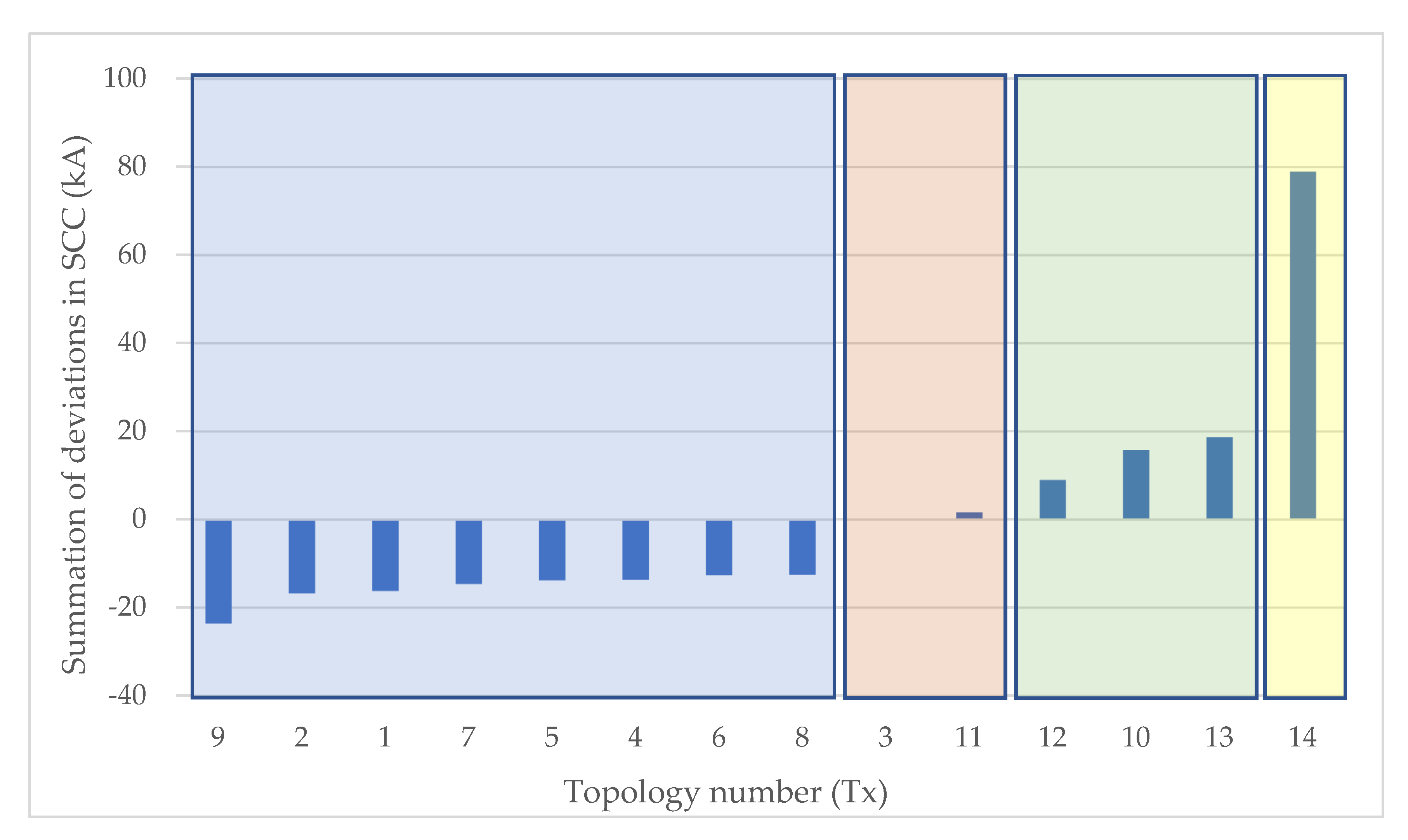
| Tx | STx (kA) | Tx | STx (kA) |
|---|---|---|---|
| 1 | −16.21 | 8 | −12.65 |
| 2 | −16.73 | 9 | −23.62 |
| 3 | 1.60 | 10 | 15.77 |
| 4 | −13.80 | 11 | −0.09 |
| 5 | −13.66 | 12 | 8.98 |
| 6 | −12.58 | 13 | 18.70 |
| 7 | −14.66 | 14 | 78.93 |
| Cluster 1 | Cluster 2 | Cluster 3 | Cluster 4 |
|---|---|---|---|
| Topology 1 Topology 2 Topology 4 Topology 5 Topology 6 Topology 7 Topology 8 Topology 9 | Topology 3 Topology 11 | Topology 10 Topology 12 Topology 13 | Topology 14 |
| Algorithm | References | |
|---|---|---|
| Algorithm | Application | |
| Modified Particle Swarm Optimization (PSO) | K. Masuda, 2010. [46] | M.M Mansour, 2007. [47] |
| Particle Swarm Optimization-Gravitational Search Algorithm (PSOGSA) | S. Z. M. Hashim, 2010. [48] | A. Srivastava, 2016. [49] |
| Harris Hawks Optimization (HHO) | A.A Heidari, 2019. [50] | J. Yu, 2020. [51] |
| Whale Optimization Algorithm (WOA) | S. Mirjalili, 2016. [52] | A. Wadood, 2019. [27] |
| Grey Wolf Algorithm (GWO) | A. Lewis, 2014. [53] | A. Korashy, 2018. [54] |
| Water Cycle—Moth Flame Algorithm (WCMFO) | S. Khalilpourazari, 2019. [45] | - |
| R | PSO | PSOGSA | HHO | WOA | GWO | WCMFO | ||||||
|---|---|---|---|---|---|---|---|---|---|---|---|---|
| TDS (s) | PS (A) | TDS (s) | PS (A) | TDS (s) | PS (A) | TDS (s) | PS (A) | TDS (s) | PS (A) | TDS (s) | PS (A) | |
| 1 | 0.18 | 3.45 | 0.05 | 9.02 | 0.20 | 1.58 | 0.18 | 2.39 | 0.14 | 3.89 | 0.14 | 3.86 |
| 2 | 0.36 | 1.47 | 0.18 | 1.01 | 0.21 | 1.11 | 0.22 | 1.00 | 0.21 | 1.00 | 0.16 | 1.33 |
| 3 | 0.40 | 1.52 | 0.15 | 1.10 | 0.20 | 2.02 | 0.24 | 2.02 | 0.24 | 2.02 | 0.25 | 1.96 |
| 4 | 0.66 | 1.54 | 0.05 | 7.07 | 0.19 | 1.30 | 0.19 | 1.35 | 0.19 | 1.33 | 0.18 | 1.30 |
| 5 | 0.14 | 2.34 | 0.25 | 1.16 | 0.21 | 1.15 | 0.23 | 1.00 | 0.22 | 1.00 | 0.22 | 1.00 |
| 6 | 0.44 | 5.14 | 0.24 | 2.02 | 0.19 | 2.34 | 0.18 | 2.40 | 0.09 | 6.28 | 0.11 | 5.65 |
| 7 | 0.23 | 3.57 | 0.26 | 1.00 | 0.20 | 2.44 | 0.25 | 1.96 | 0.24 | 2.28 | 0.22 | 2.93 |
| 8 | 0.41 | 3.11 | 0.14 | 1.79 | 0.20 | 1.99 | 0.21 | 1.89 | 0.15 | 3.57 | 0.20 | 2.43 |
| 9 | 0.21 | 4.53 | 0.28 | 1.00 | 0.20 | 2.32 | 0.19 | 2.62 | 0.22 | 2.21 | 0.10 | 6.43 |
| 10 | 0.27 | 5.03 | 0.11 | 5.95 | 0.20 | 2.58 | 0.20 | 2.51 | 0.11 | 7.22 | 0.12 | 6.38 |
| 11 | 0.28 | 2.91 | 0.05 | 7.48 | 0.20 | 2.84 | 0.14 | 2.84 | 0.14 | 3.30 | 0.12 | 3.37 |
| 12 | 0.30 | 5.41 | 0.39 | 1.09 | 0.20 | 2.20 | 0.15 | 3.37 | 0.10 | 6.50 | 0.10 | 5.94 |
| 13 | 0.16 | 7.86 | 0.34 | 3.30 | 0.20 | 3.39 | 0.15 | 3.73 | 0.06 | 9.89 | 0.05 | 9.89 |
| 14 | 0.32 | 4.57 | 0.45 | 1.00 | 0.20 | 2.38 | 0.19 | 2.31 | 0.25 | 1.99 | 0.18 | 3.25 |
| 15 | 0.10 | 6.38 | 0.53 | 1.82 | 0.20 | 2.12 | 0.17 | 2.28 | 0.09 | 4.49 | 0.06 | 6.51 |
| 16 | 0.42 | 4.05 | 0.39 | 1.52 | 0.20 | 1.59 | 0.18 | 1.87 | 0.10 | 5.11 | 0.10 | 5.11 |
| OF | 16.8236 s | 10.0170 s | 8.6590 s | 8.2953 s | 8.1858 s | 7.7457 s | ||||||
| Comparing Algorithms | The Net Gain in Total Operating Time (s) | Percentage Gain (%) |
|---|---|---|
| WCMFO/PSO | 9.0779 | 53.96 |
| WCMFO/PSOGSA | 2.2713 | 22.67 |
| WCMFO/HHO | 0.9133 | 10.55 |
| WCMFO/WOA | 0.5496 | 6.63 |
| WCMFO/GWO | 0.4401 | 5.38 |
| R | Cluster 1 | Cluster 2 | Cluster 3 | Cluster 4 | ||||
|---|---|---|---|---|---|---|---|---|
| TDS (s) | PS (A) | TDS (s) | PS (A) | TDS (s) | PS (A) | TDS (s) | PS (A) | |
| 1 | 0.10 | 5.04 | 0.10 | 4.22 | 0.14 | 3.86 | 0.07 | 3.08 |
| 2 | 0.12 | 3.53 | 0.24 | 1.79 | 0.16 | 1.33 | 0.05 | 1.91 |
| 3 | 0.22 | 1.03 | 0.14 | 2.66 | 0.25 | 1.96 | 0.06 | 4.41 |
| 4 | 0.20 | 1.00 | 0.14 | 3.70 | 0.18 | 1.30 | 0.10 | 1.10 |
| 5 | 0.11 | 3.36 | 0.12 | 3.32 | 0.22 | 1.00 | 0.07 | 1.82 |
| 6 | 0.05 | 7.67 | 0.05 | 7.53 | 0.11 | 5.65 | 0.07 | 3.51 |
| 7 | 0.12 | 4.20 | 0.15 | 3.77 | 0.22 | 2.93 | 0.16 | 3.53 |
| 8 | 0.06 | 6.09 | 0.07 | 6.46 | 0.20 | 2.43 | 0.08 | 2.38 |
| 9 | 0.08 | 5.77 | 0.19 | 2.13 | 0.10 | 6.43 | 0.13 | 3.50 |
| 10 | 0.07 | 9.99 | 0.08 | 8.51 | 0.12 | 6.38 | 0.08 | 5.46 |
| 11 | 0.14 | 1.53 | 0.23 | 1.15 | 0.12 | 3.37 | 0.05 | 3.87 |
| 12 | 0.05 | 9.07 | 0.07 | 7.33 | 0.10 | 5.94 | 0.06 | 5.66 |
| 13 | 0.20 | 1.75 | 0.32 | 1.02 | 0.05 | 9.89 | 0.05 | 5.49 |
| 14 | 0.24 | 1.03 | 0.13 | 2.94 | 0.18 | 3.25 | 0.12 | 2.71 |
| 15 | 0.06 | 8.45 | 0.09 | 6.85 | 0.06 | 6.51 | 0.12 | 1.83 |
| 16 | 0.19 | 1.53 | 0.20 | 1.32 | 0.10 | 5.11 | 0.14 | 1.15 |
| OF | 5.3431 s | 6.6272 s | 7.7457 s | 5.0519 s | ||||
| Relay | Fault Current (A) | Operating Time (s) | CTI (s) | |||
|---|---|---|---|---|---|---|
| Primary R | Backup R | Primary R | Backup R | Primary R | Backup R | |
| 1 | 5 | - | - | - | - | - |
| 1 | 14 | - | - | - | - | - |
| 2 | 4 | - | - | - | - | - |
| 3 | 1 | 0 | 0 | - | - | - |
| 4 | 16 | 17,707 | 7116 | 0.3318 | 0.5319 | 0.2001 |
| 4 | 7 | 17,707 | 2200 | 0.3318 | 0.5535 | 0.2217 |
| 5 | 3 | 10,811 | 0 | 0.3193 | - | - |
| 5 | 7 | 10,811 | 2228 | 0.3193 | 0.5487 | 0.2294 |
| 6 | 16 | 15,415 | 7051 | 0.1644 | 0.5339 | 0.3695 |
| 6 | 3 | 15,415 | 0 | 0.1644 | - | - |
| 7 | 9 | 4805 | 4805 | 0.3589 | 0.5591 | 0.2003 |
| 8 | 6 | 3699 | 3699 | 0.3165 | 0.5290 | 0.2126 |
| 9 | 11 | 19,591 | 2655 | 0.2320 | 0.4460 | 0.2140 |
| 10 | 8 | 19,378 | 2085 | 0.2877 | 0.5393 | 0.2516 |
| 11 | 13 | 3442 | 3442 | 0.3971 | 0.6008 | 0.2037 |
| 12 | 10 | 10,057 | 10,057 | 0.2884 | 0.4955 | 0.2070 |
| 13 | 15 | 5923 | 5923 | 0.4830 | 0.7231 | 0.2401 |
| 14 | 12 | 4699 | 4699 | 0.4948 | 0.6951 | 0.2003 |
| 15 | 5 | 19,177 | 5706 | 0.2308 | 0.4443 | 0.2135 |
| 15 | 2 | 19,177 | 0 | 0.2308 | - | - |
| 16 | 14 | 16,311 | 2710 | 0.3942 | 0.5953 | 0.2011 |
| 16 | 2 | 16,311 | 0 | 0.3942 | - | - |
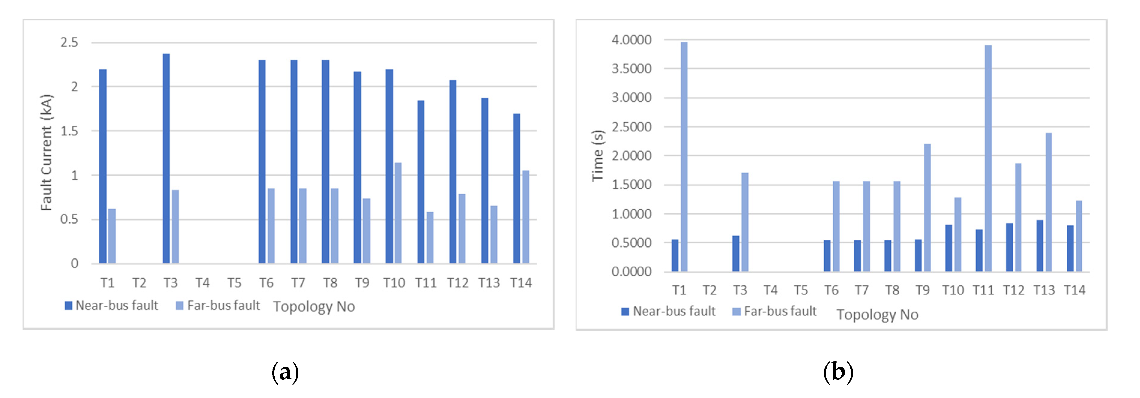
| Topology Number | R4 Current (Primary) (A) | R4 Operating Time (Primary) (s) | R7 Current (Backup) (A) | R7 Operating Time (Backup) (s) | ||||
|---|---|---|---|---|---|---|---|---|
| Near-Bus Fault | Far-Bus Fault | Near-Bus Fault | Far-Bus Fault | Near-Bus Fault | Far-Bus Fault | Near-Bus Fault | Far-Bus Fault | |
| T1 | 17,707 | 4999 | 0.3318 | 0.4872 | 2200 | 621 | 0.5535 | 3.9629 |
| T2 | - | - | - | - | - | - | - | - |
| T3 | 10,892 | 4311 | 0.4196 | 0.7130 | 2369 | 834 | 0.6236 | 1.7050 |
| T4 | 15,091 | 4263 | 0.3459 | 0.5173 | 0 | 0 | - | - |
| T5 | 15,091 | 4263 | 0.3459 | 0.5173 | 0 | 0 | - | - |
| T6 | 16,728 | 4381 | 0.3367 | 0.5119 | 2299 | 855 | 0.5372 | 1.5587 |
| T7 | 16,728 | 4381 | 0.3367 | 0.5119 | 2299 | 855 | 0.5372 | 1.5587 |
| T8 | 16,728 | 4381 | 0.3367 | 0.5119 | 2299 | 855 | 0.5372 | 1.5587 |
| T9 | 17,001 | 4425 | 0.3353 | 0.5099 | 2171 | 733 | 0.5586 | 2.2033 |
| T10 | 8659 | 3183 | 0.3946 | 0.5887 | 2193 | 1139 | 0.8159 | 1.2785 |
| T11 | 16,495 | 4368 | 0.3535 | 0.7060 | 1849 | 591 | 0.7352 | 3.9126 |
| T12 | 14,816 | 4096 | 0.3345 | 0.5242 | 2070 | 787 | 0.8430 | 1.8709 |
| T13 | 15,448 | 4210 | 0.3306 | 0.5180 | 1871 | 661 | 0.8948 | 2.3909 |
| T14 | 5633 | 2313 | 0.2346 | 0.3449 | 1694 | 1053 | 0.8037 | 1.2296 |
| Topology Number | CTI (s) | |
|---|---|---|
| Near-Bus Fault | Far-Bus Fault | |
| T1 | 0.22 | 3.48 |
| T2 | ||
| T3 | 0.20 | 0.99 |
| T4 | - | - |
| T5 | - | - |
| T6 | 0.20 | 1.05 |
| T7 | 0.20 | 1.05 |
| T8 | 0.20 | 1.05 |
| T9 | 0.22 | 1.69 |
| T10 | 0.42 | 0.69 |
| T11 | 0.38 | 3.21 |
| T12 | 0.51 | 1.35 |
| T13 | 0.56 | 1.87 |
| T14 | 0.57 | 0.88 |
© 2020 by the authors. Licensee MDPI, Basel, Switzerland. This article is an open access article distributed under the terms and conditions of the Creative Commons Attribution (CC BY) license (http://creativecommons.org/licenses/by/4.0/).
Share and Cite
Senarathna, T.S.S.; Hemapala, K.T.M.U. Optimized Adaptive Overcurrent Protection Using Hybridized Nature-Inspired Algorithm and Clustering in Microgrids. Energies 2020, 13, 3324. https://doi.org/10.3390/en13133324
Senarathna TSS, Hemapala KTMU. Optimized Adaptive Overcurrent Protection Using Hybridized Nature-Inspired Algorithm and Clustering in Microgrids. Energies. 2020; 13(13):3324. https://doi.org/10.3390/en13133324
Chicago/Turabian StyleSenarathna, Thiramuni Sisitha Sameera, and Kullappu Thantrige Manjula Udayanga Hemapala. 2020. "Optimized Adaptive Overcurrent Protection Using Hybridized Nature-Inspired Algorithm and Clustering in Microgrids" Energies 13, no. 13: 3324. https://doi.org/10.3390/en13133324
APA StyleSenarathna, T. S. S., & Hemapala, K. T. M. U. (2020). Optimized Adaptive Overcurrent Protection Using Hybridized Nature-Inspired Algorithm and Clustering in Microgrids. Energies, 13(13), 3324. https://doi.org/10.3390/en13133324