Iterative Online Fault Identification Scheme for High-Voltage Circuit Breaker Utilizing a Lost Data Repair Technique

Abstract

Most of the prior-art electrical noninvasive monitoring systems adopt Zigbee, Bluetooth, or other wireless communication infrastructure. These low-cost channels are often interrupted by strong electromagnetic interference and result in monitoring anomalies, particularly packet loss, which severely affects the precision of equipment fault identification. In this paper, an iterative online fault identification framework for a high-voltage circuit breaker utilizing a novel lost data repair technique is developed to adapt to low-data quality conditions. Specifically, the improved efficient k-nearest neighbor (kNN) algorithm enabled by a k-dimensional (K-D) tree is utilized to select the reference templates for the unintegrated samples. An extreme learning machine (ELM) is utilized to estimate the missing data based on the selected nearest neighbors. The Softmax classifier is exploited to calculate the probability of the repaired sample being classified to each of the preset status classes. Loop iterations are implemented where the nearest neighbors are updated until their labels are consistent with the estimated labels of the repaired sample based on them. Numerical results obtained from a realistic high-voltage circuit breaker (HVCB) condition monitoring dataset illustrate that the proposed scheme can efficiently identify the operation status of HVCBs by considering measurement anomalies.

1. Introduction

As a fundamental piece of electrical equipment with current breaking capacity under normal and fault conditions, the high-voltage circuit breaker (HVCB) is of great significance for power system secure operation. HVCB faults can lead to cascading failures of power grid and even cause blackouts [1]. Indicated by statistical analyzes, 80% of actual HVCB faults are caused by poor mechanical properties [2].

The identification of traditional HVCB mechanical faults mainly relies on planned maintenance [3]. With the rapid development of information communication technology (ICT) and deployment of advanced sensors, the online monitoring and intelligent diagnostic methods for HVCB have been greatly promoted. Among emerging methods, vibration signals during the closing or opening process [4], contact stroke displacements [5], and electromagnetic coil currents [6] are utilized as the distinguishing features for HVCB diagnostic methods. As the vibration signal usually shows nonlinear and nonstationarity due to the interaction of mechanical components and structures [7], the signal decomposition tools are widely utilized to extract the features in the time-frequency domain, such as the wavelet transform (WT) [8] and Fourier analysis [9]. Based on the extracted features, many classifiers for HVCB fault identification have been adopted, among which the support vector machine (SVM) is the most widely applied model [10].

Due to the limitations of network topology, geographical environment, and economic factors, most of the electrical noninvasive monitoring systems still use the distribution carrier, Zigbee, Bluetooth, or other wireless ICT with relatively poor quality. These low-cost channels are often interrupted by strong electromagnetic interference, such as over-voltage or large current surge, resulting in monitoring anomalies, which severely affect the precision of fault identification, and even invalidate the system [11,12]. Therefore, the quality of the measurements has become a realistic concern for HVCB monitoring, and exploiting the missing data to realize the accurate online diagnosis of HVCB has become a hotspot.

In [13], when processing the training set of SVM, a clustering method is used to identify the abnormal data, and the separated abnormal data are directly removed, which may destroy the continuity and integrity of the data. Reference [14] proposes two means to address the measurement anomalies: one is flagging them and the other is replacing the anomaly with the average value of the data points lying around. In [15], the abnormal data are imputed, utilizing the artificial neural network (ANN) and autoregressive exogenous input (ARX) models. In [16], the missing data are regarded as one of the outliers, which are fitted by the autoregressive integrated moving average model (ARIMA). Generally, for fault diagnosis of electrical infrastructure, e.g., HVCB, the measurements with sharp variation are prone to reveal the possible faults and should be detected in details; unfortunately, the missing sharp variation factor cannot be well characterized by time series. Some intelligent models have also been studied to deal with data with low-value density in the power systems, such as rough sets (RS) [17]. In [18], the state information of the power quality sensing device is reduced by the RS theory, and the condition estimation is realized based on the corresponding reduced set.

In state-of-the-art works, the main concern for missing data recovery is accuracy [1,2,3,4,5,6,7,8,9,10,11,12,13,14,15,16,17,18]. For realistic power grids, the number of electrical infrastructures reaches tens or hundreds of thousands, generating nearly ten or hundred million monitoring data every year. The accumulated data have already far exceeded TB (Kilobyte) level. Faced with a tremendous amount of data, the execution efficiency of the missing data recovery and the fault diagnosis program has become a challenging task, which needs to be implemented online in practical application [19].

In this paper, an online HVCB fault diagnosis method considering missing measurements is proposed. Specifically, an extreme learning machine (ELM) is utilized to estimate the missing data based on the selected nearest neighbors. The multi-class Softmax classifier is exploited to detect the most probable fault labels after the data are repaired. Loop iterations are implemented where the nearest neighbors are updated until their labels are consistent with the estimated labels of the repaired sample. The iterative scanning procedure is capable of being implemented online, owing to an efficient k-dimensional (K-D) tree data structure.

2. HVCB Condition Monitoring System

A vital foundation for condition monitoring is to select the features, which must be able to characterize the working status of the infrastructure and be measurable under existing technical conditions. In this section, the mechanical and electrical feature signals of HVCB are analyzed.

2.1. Current in the Coil

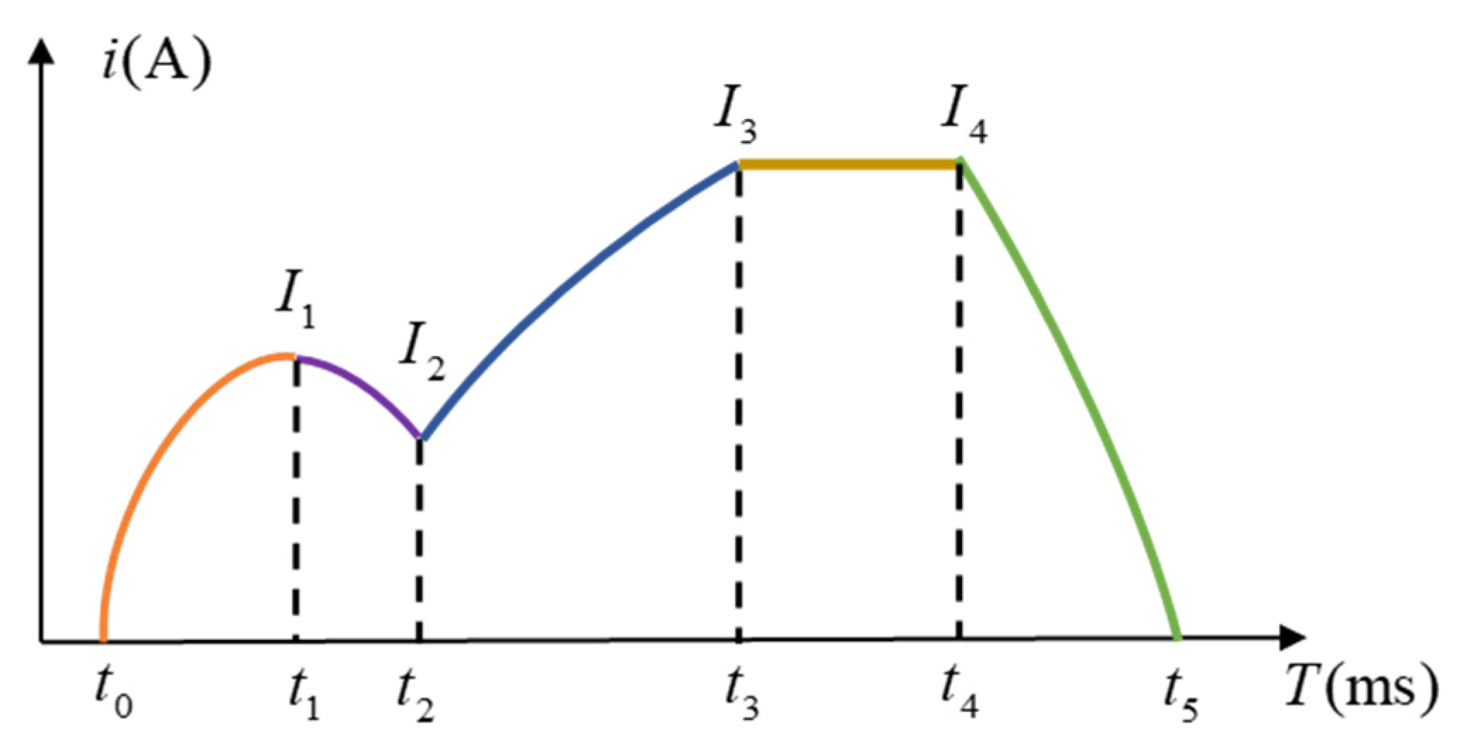
In the switch on/off process, the current flowing in the HVCB tripping and closing coil can reflect the status of the HVCB, mainly the electromagnet and its controlled parts [6]. A typical current curve in the coil is illustrated in Figure 1.

In Figure 1, t₁ and t₂ are the moments when the iron core starts and stops moving, respectively. t₃ is the timing when the coil current rises to the maximum value of steady-state current. t₄ is the cut off timing of the auxiliary contact of the circuit breaker. The duration of the four stages and the corresponding current magnitudes can reveal the voltage and resistance of the coil, as well as the core movement speed. For instance, at t₀, the coil is energized, the current grows rapidly, and the flux in the coil also rises. Before t₁, the current is not large enough to drive the core. If this stage lasts too long, it may be due to an abnormal low-coil voltage or an invalid empty stroke of iron core, etc.; alternatively, if the peak current increases simultaneously, perhaps a jammed iron core exists. When the current rises to t₁, the current value reaches the threshold and the core acts, and then the current drops. Until t₂, the iron core gradually stops, and then the core contacts with the load of the operating mechanisms. The current curve in this stage can reveal whether a jammed iron core, a deformed pole, or a failed trip exists. After t₄, the decreasing current can reflect the status of the auxiliary switch.

2.2. Vibration Signal

The mechanical vibration signal generated by the HVCB action contains valuable equipment status information.

Due to the instantaneous action of HVCB, the speed and intensity of the vibration signal are very high. The acceleration of the moving contact can reach hundreds of times of gravity acceleration; the velocity grows from the static to meters per second (m/s) in a few milliseconds (ms). Due to the change of electromagnetic force caused by the bad contact inside the HVCB, partial discharge, or the movement of conductive particles and the loosening of mechanical components, the obtained vibration signal is complex [4]. Compared with the periodic signal, the mechanical vibration of the HVCB is short. The main method is to extract its pattern characteristics by wavelet decomposition or other methods.

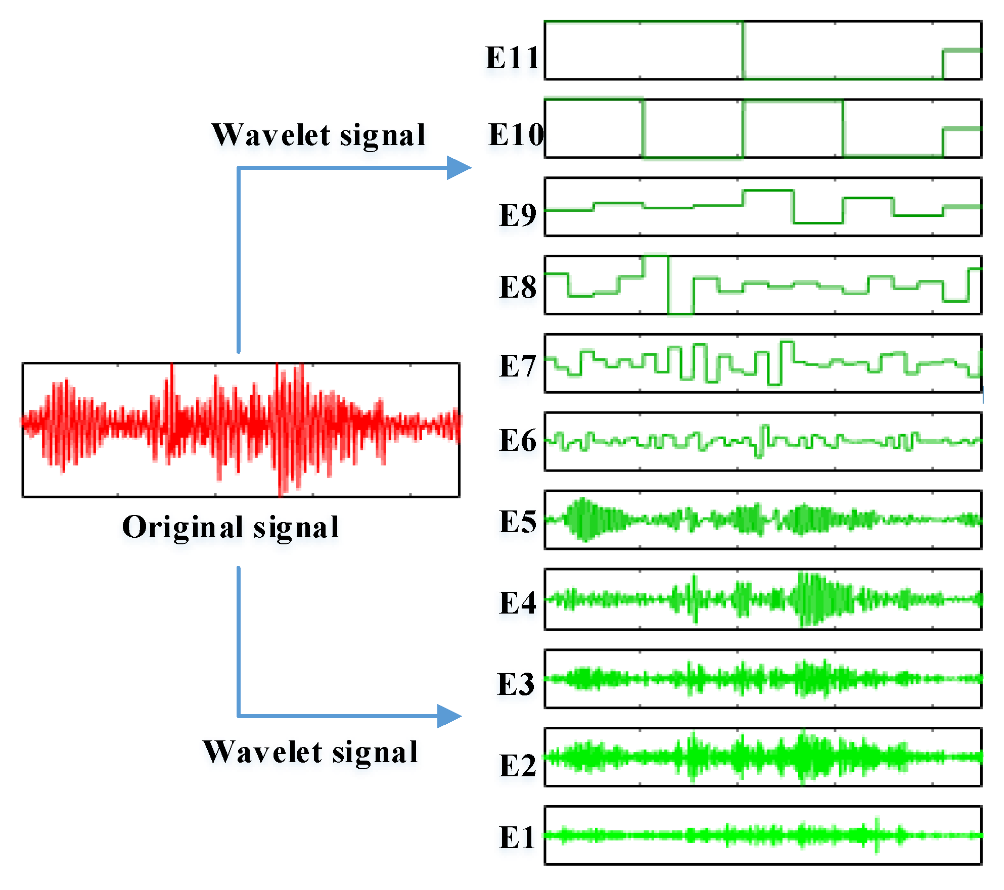
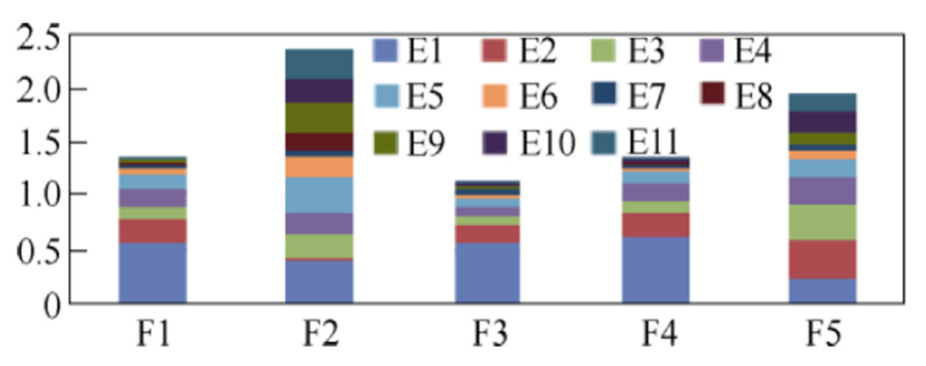
Figure 2 is a set of wavelet decomposition diagrams of a vibration signal obtained from HVCB, with 11 subwaves in total. The Harr function is adopted as the wavelet function of interest. Different subwaves represent different frequency segments of the original signal. Figure 3 is a comparison of the wavelet marginal spectrum energy of five different fault types. E1–E11 represent the marginal spectral energy of the 11 subwaves, respectively. As illustrated in Figure 3, the vibration signals of the normal and four fault types are quite distinguishable in terms of marginal spectral energy [20]. Therefore, the spectral energy of the vibration is also adopted as a feature of the HVCB monitoring.

2.3. Framework of the HVCB Condition Monitoring System

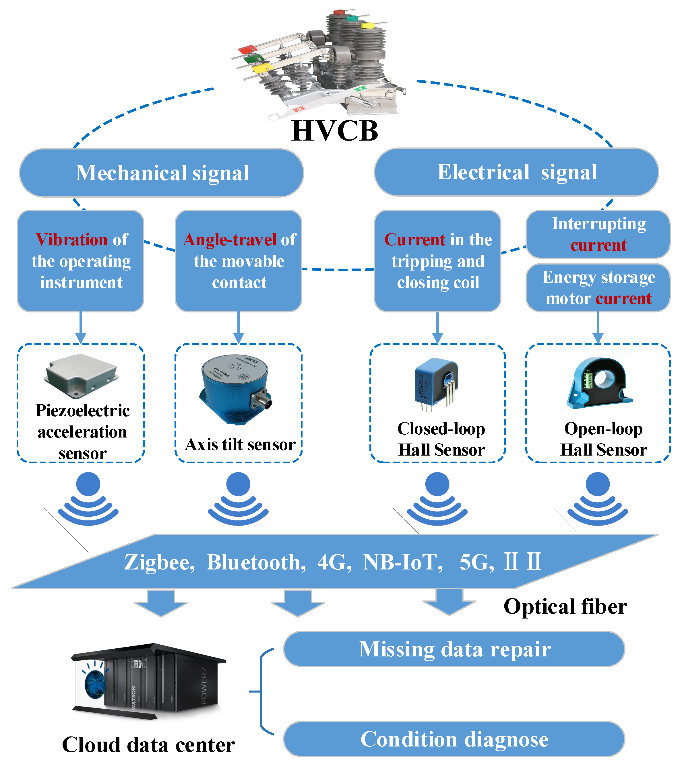
To characterize the working status of the HVCB comprehensively, a data acquisition system with multiple indicators is adopted. Specifically, in addition to the introduced coil current and vibration signal in the previous section, three supplementary indicators are utilized, including the interrupting current, the energy motor current, and the contact angle travel.

Current, vibration, and displacement are all conventional measurements, and many matured sensors are available, which are illustrated in

Table 1. Utilized features and the appropriate sensors for HVCB operation status monitoring.

Feature	Significance	Sensors
Tripping and closing coil current	Status of the mechanisms, mainly the electromagnet	Closed-loop Hall sensor
Interrupting current	Worn, aged, or deformed mechanical transmission	Open-loop Hall sensor
Energy motor current	Wear conditions of the contact
Vibration signal	Overall condition, mainly the operating mechanism	Piezoelectric acceleration sensor
Contact angle travel	Load or working state of the spring system	Axis tilt sensor

. Note that there are two kinds of Hall sensor: open-loop and closed-loop. The former adopts the principle of hall direct release, which is suitable for high current, such as the interrupting current and the motor current, while the latter follows the magnetic balance principle and fits low-current monitoring, i.e., current in the coil.

The framework of the HVCB condition monitoring system is shown in Figure 4. The system consists of distributed sensors, a communication module, and a computing center. As all the sensors are attached or close to the circuit breaker in a distributed mode, the measurements are suitable for wireless transmission in the substation using Zigbee, Bluetooth, 4G(4th Generation mobile communication), or NB-IoT(Narrow Band Internet of Things). Consider the fact that the majority of modern HV substations are configured with optical fiber, especially in China, where all the 110/220/500 kV substations have been connected with an optical Ethernet. The wireless-collected HVCB measurements in the substation are transmitted to the cloud data center through the optical fiber network. Generally, packet loss or delay dislocation are real concerns for communication systems, especially the wireless part in the substation. Therefore, in the cloud data center, a missing data repair program is deployed along with a data-driven HVCB fault diagnosis model.

3. Missing Data Repair Method

The extreme learning machine (ELM) is exploited to estimate the missing data with an extremely fast learning ability, and a k-nearest neighbor (kNN) searching algorithm is utilized to select the similar training samples, along with a k-dimensional (K-D) tree-based fast scanning technique.

3.1. kNN-Based Clustering

The kNN algorithm is a kind of supervised learning method, which is used to find neighbor samples with similar patterns [21]. Based on the basic premise that the faults of the same equipment are of a similar data mode, this paper adopts the improved kNN algorithm to repair the lost measurements of HVCB condition monitoring. After receiving a test sample with lost measurements to be repaired, we find the closest K samples in the historical database, and then synthesize the information of the K training samples to estimate the lost part. In order to reveal the relevance among different monitoring indicators, the similarities of samples are measured in terms of Manhattan distances weighted by the negative exponential of the related coefficient.

If there are N HVCB monitoring sample pairs with m features in each pair $x_i={\left[x_{i1},x_{i2},\cdots ,x_{im}\right]}^T\left(1\le i\le N\right)$, the correlation degree of the p-th and q-th feature values ${\rho }_{pq}$ can be obtained by [22]:

$${\rho }_{pq}=\frac{\frac{1}{N-1}{\displaystyle \sum _{i=1}^N\left(x_{ip}-{\mu }_p\right)\left(x_{iq}-{\mu }_q\right)}}{\sqrt{\frac{1}{N-1}{\displaystyle \sum _{i=1}^N{\left(x_{ip}-{\mu }_p\right)}^2}}\sqrt{\frac{1}{N-1}{\displaystyle \sum _{i=1}^N{\left(x_{iq}-{\mu }_q\right)}^2}}}$$

(1)

where $\mu$ is the average of the corresponding feature, and ${\rho }_{pq}$ is the range of the related coefficient from −1 to +1. The −1 means a strong negative correlation between the two features. The +1 means a strong positive correlation, while 0 indicates no correlation.

Assume that the test sample $x_i$ lacks the p-th (1 ≤ p ≤ m) feature measurement $x_{ip}$, the Manhattan distance weighted by the negative exponential of the related coefficient between training sample i and test sample j can be expressed as [23]:

$$d_{ij|p}={\displaystyle \sum _{q=1}^m{e}^{-\left|{\rho }_{pq}\right|}\cdot \left|x_{iq}-x_{iq}\right|}, p\ne q$$

(2)

The spatial distances of measurements are weighted by the correlation coefficients. For features highly correlated with the feature of the missing value, smaller weights are assigned. In this way, the test sample is prone to approach the training samples with similar measurements on strong correlated features.

3.2. ELM for Data Estimation

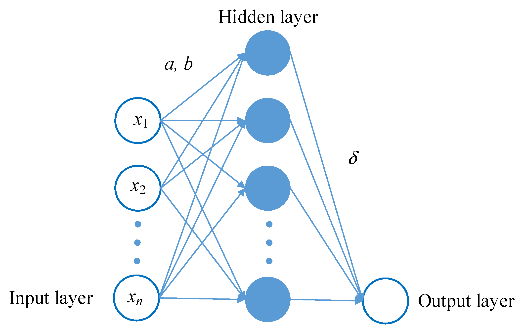
The ELM is a single-hidden-layer feedforward neural network (SLFN) with fast learning speed and excellent generalization. The ELM randomly sets the input weights and biases, which are not required to be tuned iteratively in the training procedure, thus greatly saving the overall training workload.

As can be seen in Figure 5, given a dataset with N samples ${\left\{\left(x_i,y_i\right)\right\}}_{i=1}^N$, where $x_i\in ℝ$ and $y_i\in ℝ$ are inputs and targets respectively, a K-hidden unit ELM with activation function $\varphi (·)$ approximates the N samples without error, as follows [24]:

$$y_i={\displaystyle \sum _{i=1}^K{\beta }_i}\varphi \left(a_i\cdot x_j+b_i\right), \left(j=1,2,\cdots ,N\right)$$

(3)

where $a_i={\left[a_{i1},a_{i2},\cdots ,a_{in}\right]}^T$ is the vector of the weights connecting the hidden unit i and the input units of the ELM, ${\delta }_i={\left[{\delta }_{i1},{\delta }_{i2},\cdots ,{\delta }_{im}\right]}^T$ is the vector of weights connecting the hidden unit i and the output units, $b_i$ is the bias of the hidden unit i, and $\varphi \left(a_i\cdot x_j+b_i\right)$ is the output of the hidden unit i with respect to $x_i$. Equation (3) can be expressed in compact form: $H\delta =Y$, where $H$ is the output matrix of the ELM hidden layers, and

$$H=\left[\begin{array}{ccc}\varphi \left(a_1\cdot x_1+b_1\right)& \cdots & \varphi \left(a_K\cdot x_1+b_K\right)\\ ⋮& & ⋮\\ \varphi \left(a_1\cdot x_N+b_1\right)& \cdots & \varphi \left(a_K\cdot x_N+b_K\right)\end{array}\right]$$

(4)

The column i of matrix $H$ corresponds to the output vector of the hidden unit i with respect to input $x_i={\left[x_{i1},x_{i2},\cdots ,x_{in}\right]}^T$. In addition, $\delta$ is the output weight matrix and $Y$ is the target matrix.

With the randomly set $a_i$ and $b_i$, the output matrix $H$ can be determined uniquely; consequently, the approximated parameters $a_i$, $b_i$, and $\delta$ can be acquired by:

$$\Vert H\left(a_1^{*},\cdots ,a_K^{*},b_1^{*},\cdots ,b_K^{*}\right)\delta -T\Vert =\underset{\delta }{\min }\Vert H\left(a_1,\cdots ,a_K,b_1,\cdots ,b_K\right)\delta -T\Vert$$

(5)

Training an ELM is actually equivalent to searching the unique minimal norm least-square scheme of the linear model in Equation (4), i.e.,

$${\delta }^{*}=H^{+}Y$$

(6)

where $H^{+}$ is the Moore–Penrose generalized inverse (MPGI) of $H$, which can be obtained through algorithms such as the singular value decomposition (SVD) [24].

The conventional gradient-based ANN models like the BP (Back Propagation) network are involved with iterative time-consuming training. The ELM achieves extremely efficient training due to simple matrix transformation and can always guarantee global optimality. In addition, it has many advantages, such as avoiding overtraining.

3.3. K-D Tree-Based Fast Scanning Technique

If the conventional linear scanning technique is utilized to locate the k-closest samples, the efficiency is not capable of meeting the requirements of online identification. In this paper, an efficient searching structure named the K-D tree is introduced.

3.3.1. Building a K-D tree

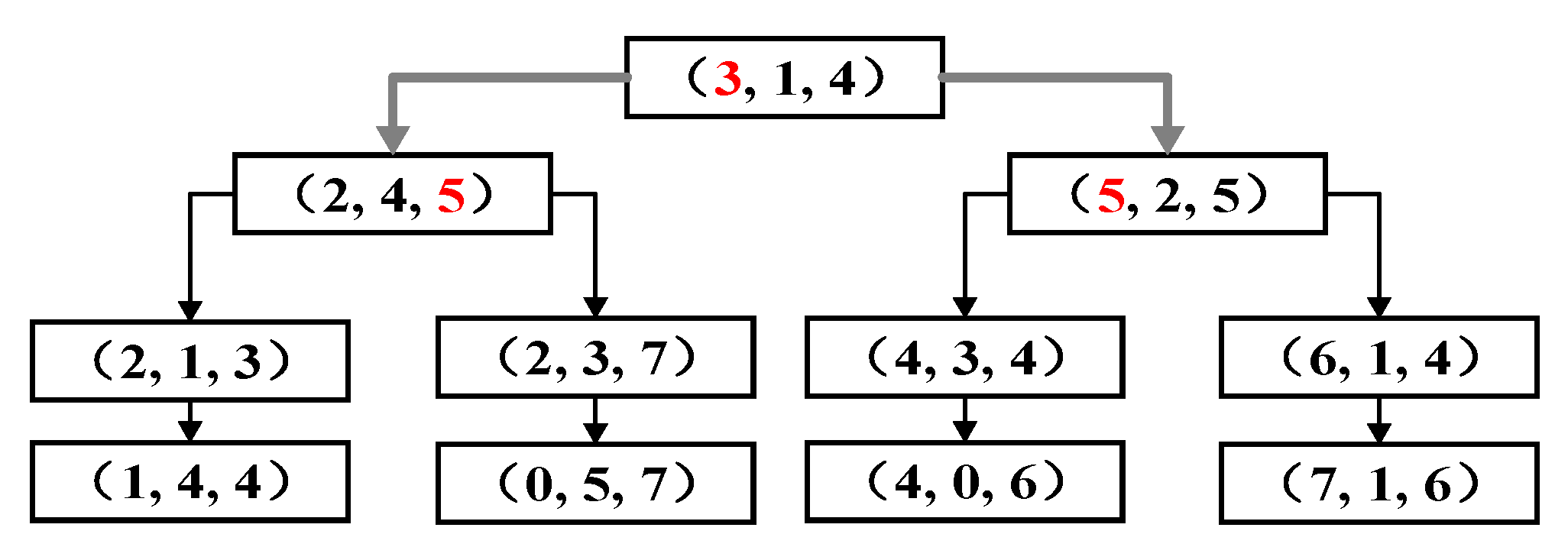
HVCB monitoring usually covers more than 10 indices; therefore, HVCB condition monitoring is a high-dimensional data space. The K-D tree is an enhanced data structure to segment data space with k dimensions and speedup the searching efficiency in it [25]. Figure 6 illustrates a 3-dimensional dataset to explain the formation of a K-D structure, including three specific steps.

Step 1: Calculate the data variance of each feature or dimension, and select the dimension with the maximum variance value as the split dimension (SD). Generally, a larger variance means a better diversity of data in this dimension. Dividing samples in the direction indicated by the maximum variance can effectively balance the overall tree.

Step 2: Sort the data samples based on the values of the SD; find the pivot point with the most intermediate value on the SD. In Figure 6, the pivot point data of the SD are highlighted in red font.

Step 3: Divide the whole dataset on the SD to form two branches of K-D trees. When the size of the branched tree is less than the preset maximum leaf node, which is 2 in Figure 6, stop generating branches of K-D trees. Otherwise, return to step 1.

Each node of the obtained structure is a k-dimensional binary tree. All nonleaf nodes can be regarded as a hyperplane for space division. Through nonoverlapping hierarchical division of the search space, an index structure suitable for efficient data searching is established.

3.3.2. Neighborhood Searching

For structured storage, each HVCB monitoring data sample is of k indices and placed on a node of K-D tree.

It has been proved in Reference [25] that the complexity of the neighborhood searching in a K-D tree structure is O(logn) (n is the dimension of the data space), which significantly surpasses the conventional linear scanning algorithm with O(n) complexity [26]. The K-D tree-based neighborhood searching strategy consists of three steps.

Step 1: Locate the leaf nodes of the samples along the K-D tree, obtain the closest data point, and put all nodes on the searching route into a queue.

Step 2: Check whether the distance from the data point in the queue to the test sample is closer than that from the test sample to the closest data point. If not, remove the node out of the queue and duplicate step 2 until the queue becomes empty; then terminate the search process. Otherwise, move forward to step 3.

Step 3: Update the closest data point and add its offspring nodes to the queue. Then, go back to step 2.

4. Softmax Classifier for HVCB Status Identification

The essence of HVCB condition identification is to identify its operation label based on a series of measurements, which is a multi-class classification problem. First of all, there is no strict one-to-one correspondence between the external measurements with limited dimensions and the operation state. Generally, multiple possible states exist under the observations theoretically. The task is to find the most probable state, which is a probability problem. In addition, the rules of classification cannot be given in advance, and some machine learning models are required to train the rules from historical data. This section introduces a Softmax classifier for the HVCB condition diagnosis task.

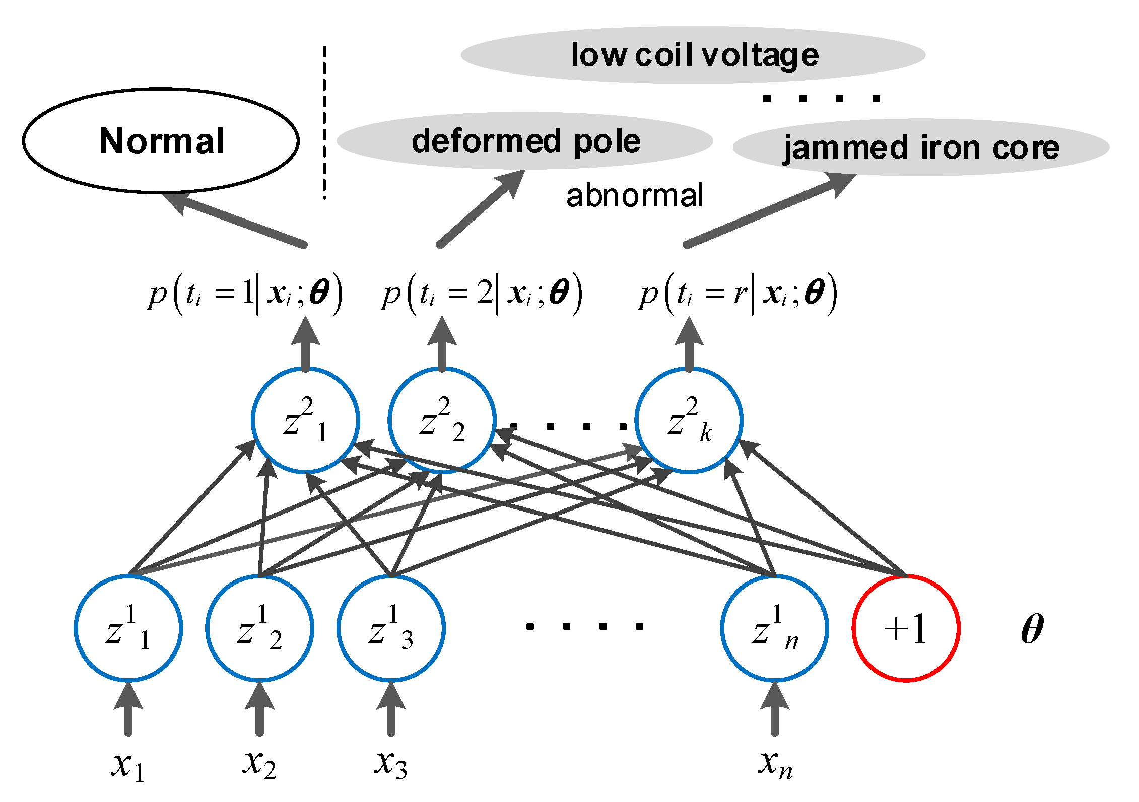
As illustrated in Figure 7, the Softmax classifier is actually a two-layer ANN, which quantifies the probability value of classifying a certain input sample to each predefined label and select the label with the maximal probability. Given an HVCB measurement input $x_i={\left[x_{i1},x_{i2},\cdots ,x_{in}\right]}^T$, $t_i$ is the label which can be assigned as r values. As shown in Equation (6), the Softmax classifier can give a vector with r dimensions corresponding to r calculated probabilities [27].

$$h_{\mathit{\theta }}\left({\mathit{x}}_i\right)=\left[\begin{array}{c}p\left(t_i=1|{\mathit{x}}_i;\mathit{\theta }\right)\\ p\left(t_i=2|{\mathit{x}}_i;\mathit{\theta }\right)\\ ⋮\\ p\left(t_i=r|{\mathit{x}}_i;\mathit{\theta }\right)\end{array}\right]=\frac{1}{{\displaystyle \sum _{j=1}^r{e}^{{\mathit{\theta }}_j^T{\mathit{x}}_i}}}\left[\begin{array}{c}{e}^{{\mathit{\theta }}_1^T{\mathit{x}}_i}\\ e^{{\mathit{\theta }}_2^T{\mathit{x}}_i}\\ ⋮\\ e^{{\mathit{\theta }}_i^T{\mathit{x}}_i}\end{array}\right]$$

(7)

where ${\theta }_1,{\theta }_2,\cdots ,{\theta }_r\in {ℝ}^{r\times 1}$ are the weights to be trained, ${\displaystyle \sum _{j=1}^r{e}^{{\mathit{\theta }}_j^T{\mathit{x}}_i}}$ is utilized to normalize the probability vector, and the probability of sorting input $x_i$ into label j is:

$$p\left(t_i=j|{\mathit{x}}_i;\mathit{\theta }\right)=\frac{e^{{\mathit{\theta }}_j^T{\mathit{x}}_i}}{{\displaystyle \sum _{l=1}^r{e}^{{\mathit{\theta }}_l^T{\mathit{x}}_i}}}$$

(8)

For supervised learning with a labeled dataset, the specific label dimension of the Softmax output is assigned as value 1 and other dimensions are set as value 0.

The indicator function $1\{\cdot \}$ is introduced to express the cost function of Softmax classification:

$$1\{t_i=j\}=\{\begin{array}{c}1, if t=j\\ 0, if t\ne j\end{array}$$

(9)

The process of training the Softmax model is actually to optimize the parameter θ. The better the θ is trained, the better the classification effect can be achieved. Generally, the cross entropy index is utilized to measure the effect of model classification. Minimizing of the cross entropy (CE) value is equivalent to the process of improving Softmax classification accuracy continuously. The loss function is:

$$J\left(\mathit{\theta }\right)=-\frac{1}{m}\left[{\displaystyle \sum _{i=1}^m{\displaystyle \sum _{j=1}^{r}1\left\{t_i=j\right\}}\log \frac{e^{{\mathit{\theta }}_j^T{\mathit{x}}_i}}{{\displaystyle \sum _{l=1}^r{e}^{{\mathit{\theta }}_l^T{\mathit{x}}_i}}}}\right]$$

(10)

There is no closed method to minimize J(θ). Generally, an iterative optimization algorithm, such as the gradient descent method, is used instead. For each parameter of Equation (9), the partial derivative is obtained:

$$\frac{\delta J\left(\mathit{\theta }\right)}{\delta {\theta }_j}=-\frac{1}{m}{\displaystyle \sum _{i=1}^m\left\{x_i\left[1\left\{t_i=j\right\}-p\left(t_i=j|x_i;\mathit{\theta }\right)\right]\right\}}$$

(11)

By substituting the above partial derivative into the gradient descent method, the J(θ) can be minimized. However, the obtained θ is not unique due to the nonconvexity of Equation (9) [27]. To address the nonconvexity, a weight decay term $\frac{\lambda }{2}{\displaystyle \sum _{i=1}^r{\displaystyle \sum _{j=0}^n{\theta }_{ij}^2}}$ is added to the cost function, then the training procedure of a Softmax classifier can be abstracted as in [28]:

$$\mathit{\theta }*=\underset{\mathit{\theta }}{\arg \min }\left(-\frac{1}{m}{\displaystyle \sum _{i=1}^m{\displaystyle \sum _{j=1}^{r}1\left\{t_i=j\right\}}\log \frac{e^{{\mathit{\theta }}_j^T{x}_i}}{{\displaystyle \sum _{l=1}^r{e}^{{\mathit{\theta }}_l^T{x}_i}}}}+\frac{\lambda }{2}{\displaystyle \sum _{i=1}^r{\displaystyle \sum _{j=0}^n{\theta }_{ij}^2}}\right)$$

(12)

In a gradient descent framework, the unique optimal Softmax weight θ can be calculated by iterative BP algorithms.

5. Procedure of Iterative HVCB Diagnosis Utilizing Repaired Data

In the HVCB fault identification framework integrated with the lost data repair technique, the k-NN algorithm is adopted to gather a set of similar samples, and then the ELM is utilized to establish a map from the sample data to the measurement in terms of the dimension or feature with lost data. The ELM is capable of calculating or repairing a value for the lost feature with a satisfactory speed. The Softmax network is exploited to calculate the probability of the sample of interest being classified to each of the preset labels. In this way, preliminary or raw estimated fault labels subject to the repaired dataset are obtained on the basis of which the sample space is reconfigured and the k-NN and ELM are used to estimate the lost data again. In this way, the fault labels of the neighbor samples are iterated until they are in accordance with the detected fault labels of the test samples.

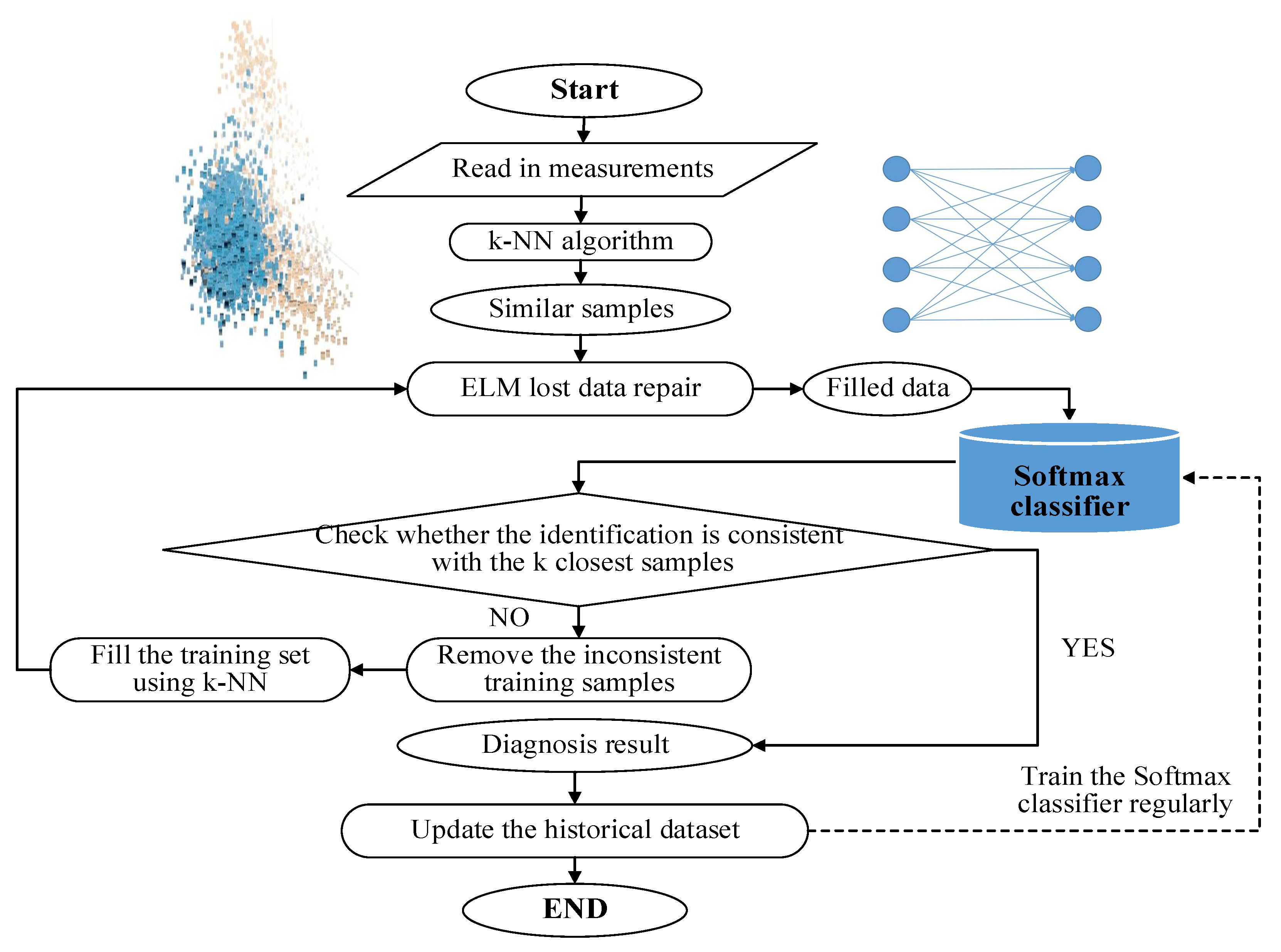
The flow chat of the proposed HVCB fault identification method based on a repaired dataset is illustrated in Figure 8, including the following five steps:

Step 1: Read in the HVCB condition monitoring data, including coil current, interrupting current, motor current, vibration signal, and angle travel of the contact, etc via the Internet of Things from the sensors deployed on HVCBs. Run the data check program to scan the measurements. If the data are complete, call the trained Softmax classifier to identify the most probable condition label. If certain data are lost, run to Step 2.

Step 2: Call the k-NN algorithm to select N training samples with the most similar measurements on strong correlated features, and run the ELM to repair the lost data based on the sample data. Then, call the trained Softmax classifier to identify the fault labels.

Step 3: Check whether the identification result is in accordance with the fault labels of the k-closest training samples. If not, forward to step 4, otherwise, jump to step 5.

Step 4: Remove the samples that are inconsistent with the identification label of the repaired data, and use the k-NN algorithm to supplement the required samples and establish an updated training set with N size again. Then, go back to step 2.

Step 5: After the above implementations, store the sample with final repaired data into the historical sample dataset along with its identification result. The Softmax classifier is trained regularly with the latest version of the historical labeled sample dataset.

Through the above iterative cleaning and maintenance mode, the quality of fault identification database of HVCB can be continuously improved against metering anomalies.

6. Realistic Case Studies

6.1. Case Description

To support the online HVCB fault identification, a labeled training set is established based on sample data obtained from both the laboratory and real operation. Specifically, defective or failure HVCBs are detected during intended fatigue tests or condition-based maintenance; the corresponding fault types are confirmed and their historical condition measurements are called. In general, 3759 pairs of complete HVCB condition monitoring data are obtained from the State Grid Corporation of China (SGCC). Note that the HVCB measurements include point-by-point mechanical vibration energy spectrum and coil current signals, and the input feature is an 8-dimensional vector. All the fault labels include loose joint pin (F1), loose connecting bolt (F2), jammed closing release (F3), lower coil voltage (F4), stuck auxiliary switch contact (F5), as well as normal (N). The samples with lost data are generated by random data deletion.

6.2. Accuracy Validation

In order to fully exploit the training data and illustrate the effects, fault identification precisions of different methods are compared under a leave-one-out cross validation (LOM) framework [29]. The competition classifiers include the Softmax, multi-class SVM [10,13], as well as RS [17,18]. The studied missing data repair techniques are the proposed k-NN combined with ELM, k-NN combined with simple average computing, and ARIMA [16]. The fault identification precisions of methods with different configurations are shown in

Table 2. Fault identification precisions of different methods.

Fault Type	Training Sample	Softmax (Complete)	Softmax (Lost)	k-NN (ELM)+ Softmax (Lost)	k-NN (ELM)+ Multi-Class SVM (Lost)	k-NN (Average) +Softmax (Lost)	ARIMA +Softmax (Lost)	RS (Complete)	RS (Lost)
F1	623	86.3%	75.8%	84.2%	81.3%	79.5%	80.3%	81.8%	71.8%
F2	656	87.6%	70.6%	88.6%	84.6%	82.3%	83.9%	77.2%	68.6%
F3	614	86.3%	68.4%	86.5%	83.7%	80.2%	79.5%	82.6%	65.4%
F4	641	90.8%	69.8%	87.2%	82.7%	78.4%	83.4%	79.7%	66.8%
F5	689	85.4%	70.2%	82.4%	78.9%	72.6%	74.6%	81.9%	63.2%
N	536	92.6%	76.9%	90.2%	85.2%	83.8%	82.9%	85.8%	70.9%
Remarks		The best results		The proposed results					The worst results

.

As can be seen from Table 2, the precision of the Softmax classifier is 85.4–92.6%, which is obviously higher than the RS method (77.2–85.8%), based on complete measurements. After the data are randomly deleted, the precisions of the Softmax and RS methods are reduced to 68.4–75.8% and 63.2–71.8%, respectively. It can be concluded obviously that the diagnosis models are highly sensitive to data integrity. As the utilized vibration energy spectrum and the current indices are all key features for operation status characterizing of HVBC, the absence of any attribute affects the accuracy greatly.

By utilizing the proposed lost data repair technique (kNN + ELM), the precision of the Softmax classifier can be restored to 82.4–90.2%, which is only a small precision decline with subject to data missing. It is validated that the proposed data-driven iterative framework is capable of meeting the application requirements, which minimizes the impact of one or several data defects on the identification precision.

Adopting the k-NN integrated ELM data repair technique and the multi-class SVM classifier, the obtained precision is 78.9–85.2%. Compared with the precision of the proposed Softmax classifier, there is about a five-percent decrease in accuracy. Because the SVM is a kind of binary classifier, multiple SVM networks need to be cascaded or stacked to fit multi-class classification problems, such as this HVCB fault identification case, which is prone to enlarge the error to some extent [10,13].

If the lost data are approximated by computing the average of samples searched by k-NN in the dimension of interest, the Softmax accuracy decreases to 72.6–83.8%. As can be seen, though a certain correlation indeed exists in the sample data, modeling it in linear form results in significant errors. The nonlinear ELM adopted in this paper achieves a better data recovering effect compared with replacing the anomaly with the average value of the data points lying before and after it [14]. 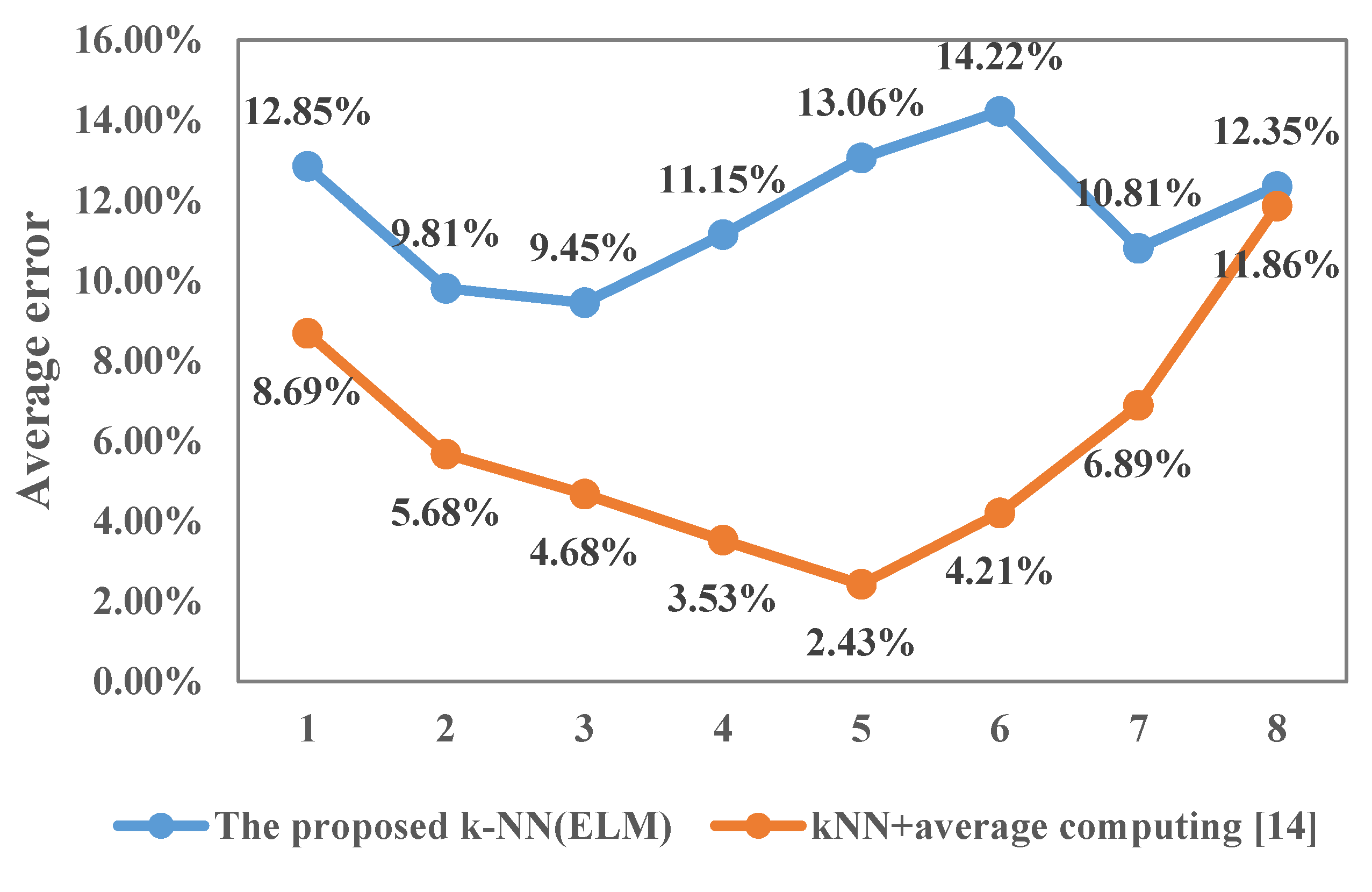Figure 9 illustrates the relationship of lost data estimation error and the number of selected neighborhood samples in the k-NN framework. For the ELM estimator, when insufficient or excessive samples are selected, the prediction error increases, and the most appropriate number of neighborhood samples is 25 (average error = 2.43%). For the average computing estimator, the obtained average error has been fluctuating around 10%.

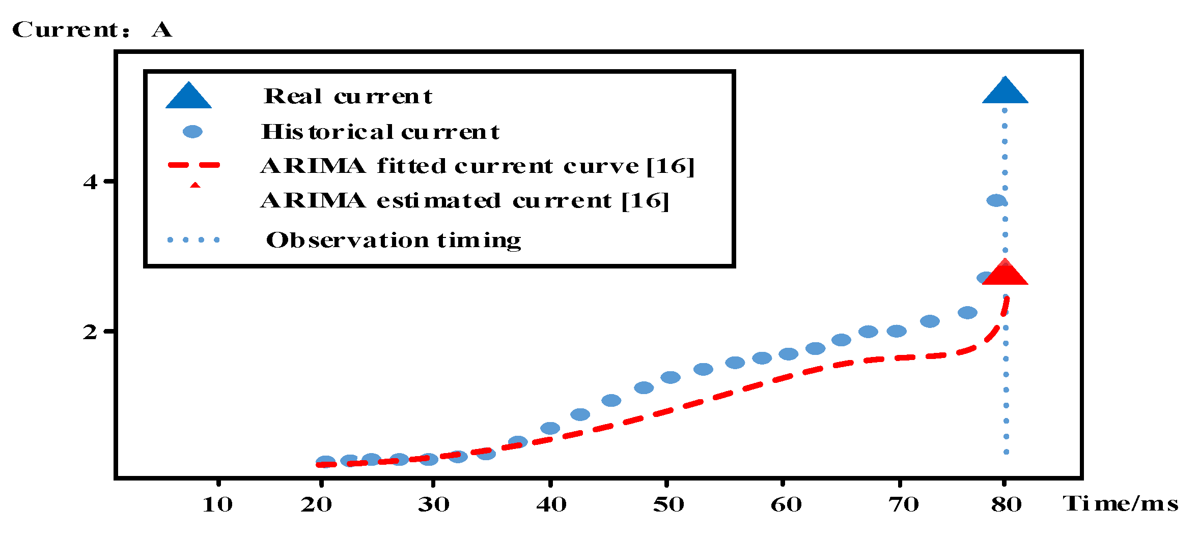
Moreover, if the ARIMA time series analysis method is used for missing data estimation, i.e., extrapolation estimation based on some measurements before data missing timing, then Softmax is still used for fault diagnosis. The corresponding precision is 74.6–83.4%, obviously lower than that of the proposed k-NN (ELM) repair technique. Figure 10 illustrates a sample of data repair using ARIMA [16]. As can be seen, due to a mechanical jam fault, the spring load torque increases, and the energy storage motor current increases sharply. If the historical current values are used for extrapolation prediction, the prediction curve of ARIMA fits the historical data in normal state too much, resulting in an over-conservative final result [16]. Compared with the time series method, k-NN is a global data searching and analysis method, which breaks the mandatory temporal causal relationship, and thus achieves better abnormal detecting ability.

6.3. Searching Efficiency Validation

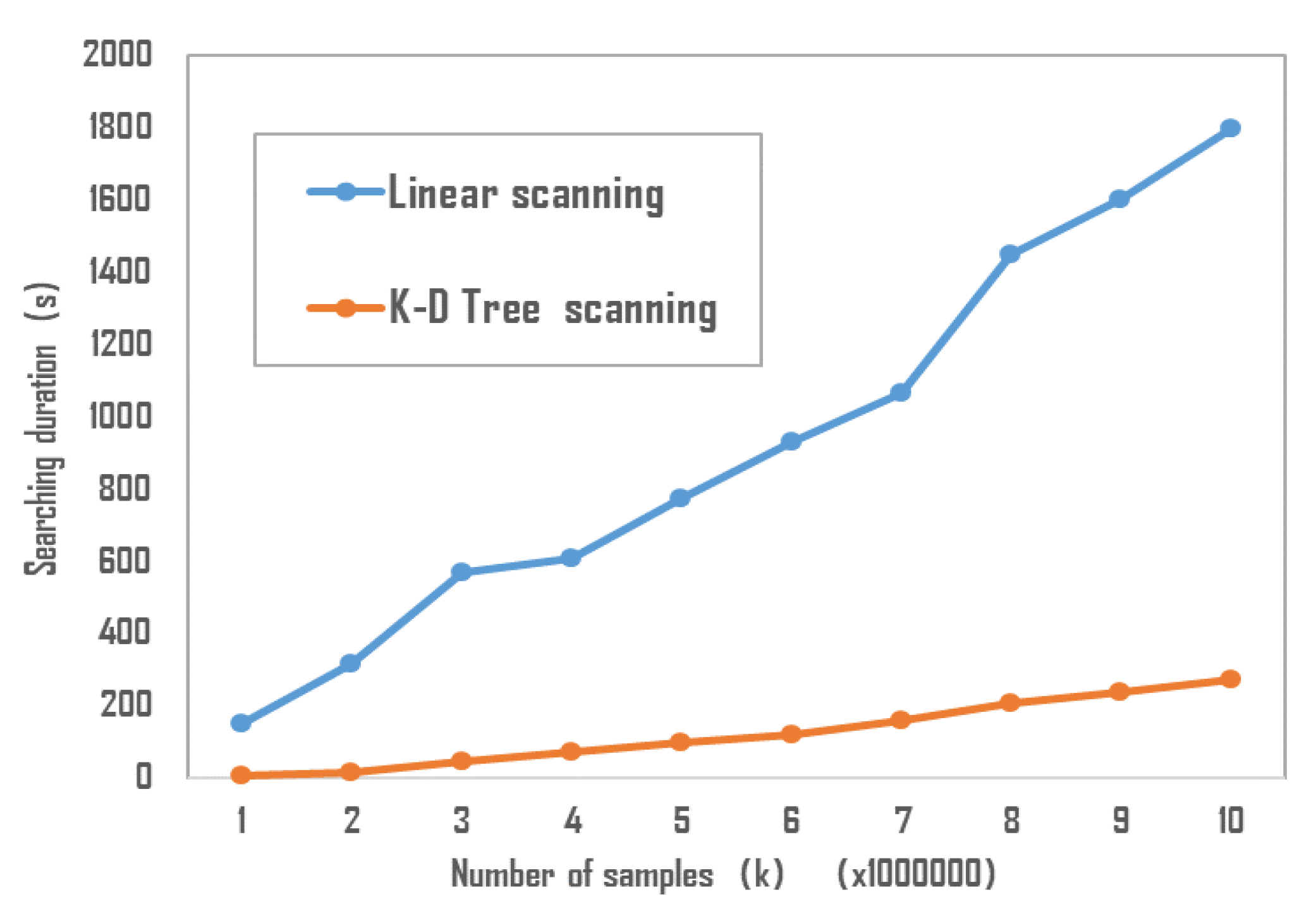
Figure 11 compares the relationship between the neighborhood sample size (K value in the k-NN framework) and the CPU (Central Processing Unit) time of the K-D tree-based and conventional linear scanning algorithms. The comparison is implemented on a dataset with 8-dimensional HVCB condition monitoring dataset in terms of the Manhattan distance. It can be illustrated that for the K-D tree-based structure, the search time of neighborhood samples increases slowly with the growing sample size. However, for the benchmark linear scanning, the time increases rapidly with the growing dataset size. Therefore, the proposed K-D tree scanning has a significant advantage when applied for online fault identification of HVCB with large scale measurements.

7. Conclusions

In this paper, a HVCB fault identification framework considering lost data is proposed, where the k-NN method is adopted to gather similar samples, and then the ELM is utilized to reconstitute the lost data. The Softmax classifier is exploited to estimate the most probable condition status of the repaired data. A loop is implemented where the fault types of the neighbor samples are iterated until they are consistent with the fault labels of the samples. In the proposed framework, the sample searching efficiency is greatly enhanced by adopting a K-D tree scanning strategy and the lost data can be repaired in a nonlinear way by ELM without iterative BP computations. Moreover, the time-consuming classifier training is implemented in advance offline; therefore, the online efficient condition monitoring of HVCB with anomaly measurements can be achieved.

With the development of the Internet of Things, exploitation of the potential value of defective data due to inadequate collection or transmission infrastructure is a common requirement for many data-driven application scenarios. Therefore, the proposed method has a broad prospect of application.