Article

Analysis of Different Neural Networks and a New Architecture for Short-Term Load Forecasting

College of Electrical Engineering and Information Technology, Sichuan University, Chengdu 610065, China
*
Author to whom correspondence should be addressed.
Energies 2019, 12(8), 1433; https://doi.org/10.3390/en12081433
Submission received: 22 January 2019 / Revised: 30 March 2019 / Accepted: 9 April 2019 / Published: 14 April 2019
(This article belongs to the Section F: Electrical Engineering)

Abstract

:
Short-term load forecasting (STLF) has been widely studied because it plays a very important role in improving the economy and security of electric system operations. Many types of neural networks have been successfully used for STLF. In most of these methods, common neural networks were used, but without a systematic comparative analysis. In this paper, we first compare the most frequently used neural networks’ performance on the load dataset from the State Grid Sichuan Electric Power Company (China). Then, considering the current neural networks’ disadvantages, we propose a new architecture called a gate-recurrent neural network (RNN) based on an RNN for STLF. By evaluating all the methods on our dataset, the results demonstrate that the performance of different neural network methods are related to the data time scale, and our proposed method is more accurate on a much shorter time scale, particularly when the time scale is smaller than 20 min.

1. Introduction

Accurate short-term load forecasting (STLF) can play a significant role in power construction planning and power grid operation, and also has crucial implications for the sustainable development of power enterprises. STLF can predict future loads for minutes to weeks. Because of the nonlinearity, non-stationarity, and non-seasonality of STLF, it is very challenging to predict accurately. Inaccurate load forecasting may increase operating costs [1]. By contrast, with an accurate electric load forecasting method, fundamental operating functions, such as unit maintenance, reliability analysis, and unit commitment, can be operated more efficiently [2]. Thus, it is essential for power suppliers to build an effective model that can predict power loads, accomplish a balance between production and demand, reduce production costs, and implement pricing schemes for various demand responses. According to the length of the forecast period, power load forecasting is divided into four categories: long-term load forecasting, medium-term load forecasting, STLF, and ultra-STLF [3].
There have been many efforts to develop accurate STLF; many methods have been propsoed [4,5,6,7,8,9,10,11,12,13,14,15,16]. In much earlier works, researchers attempted to forecast load precisely using a mathematical statistics approach. The most representative is the regression analysis approach [4], which uses a set of functional linear regression models. In [5], the authors used the Kalman filter to develop a very short-term load predictor, and the Box–Jenkins autoregressive integrated moving average approach was proposed in [6]. In [17], the relationships between demand and driver variables were evaluated by using semi-parametric additive models. Additionally, in [18], the authors came up with a new SVD-based exponential smoothing formulation. Based on linear regression and patterns, an univariate models were proposed for 34 daily cycles of a load time series in [19]. In [20], by combining a Bayesian neural network with the hybrid Monte Carlo algorithm, the authors assumed a new model for STLF. Modified artificial bee colony algorithm, extreme learning machine, and the wavelet transform were combined to construct a novel STLF method in [21].
However, mathematical statistics approaches are based on linear analysis; thus, it is difficult for them to predict nonlinear and non-stationary problems. For better learning of nonlinear features, machine learning is a good approach. Two broad categories of methods exist: support vector regression (SVR) and artificial neural networks (ANNs). In the SVR approach, a generic strategy for STLF based on the SVR has been proposed [22,23,24,25]. In this method, there are two considerable improvements to SVR-based load forecasting methods: the procedure for generating model inputs and the subsequent model input was selected by feature selection algorithms. By combining SVR with other algorithms, many hybrid methods have been proposed. An SVR model combined with the differential empirical mode decomposition algorithm and autoregression was proposed in [26,27,28], and provides higher accuracy and interpretability, and better generation ability. To extend the SVR method, a chaotic genetic algorithm was presented to improve forecasting performance in [29]. In [30,31], the authors combined support vector machines (SVMs) with a genetic algorithm, and combined SVR with ant colony optimization to forecast the system load. In [32],an attempt based on double seasonal exponential smoothing was used for STLF. Besides these studies, in [7], in order to achieve better regression and forecasting performance, the proposed SVR-based STLF approach, a supervised machine learning approach with the preprocessing of input data is required. Simultaneously, STLF models were developed using fuzzy logic and an adaptive neuro-fuzzy inference system [33], with efficient load forecasting and has been the alternative approach for STLF in Turkey.
For ANNs, the backpropagation neural network (BPNN) was the first ANN method used for load forecasting. In [34], the authors presented a BPNN approach with a rough set for complicated STLF with dynamic and nonlinear factors to enhance the performance of predictions. By combining a Bayesian neural network and BPNN, Ningl et al. [35] proposed a Bayesian-backpropagation method to forecast the hour power load of weekdays and weekends. Based on the BPNN, the authors discussed the relationship between the daily load and weather factors in [36]. Because the BPNN is a type of feedforward ANN, it cannot learn the features of time sequential data, but power load data can be considered as sequential data. Recurrent neural networks (RNNs) have been introduced into STLF. In [37,38,39,40], the authors proposed using an RNN to capture a compact and robust representation. A multiscale bi-linear RNN was proposed for STLF [41]. Additionally, a long-short term memory (LSTM) network as a type of more complex RNN has been used in STLF [42,43,44]. However, the performance of LSTM is not very effective.
Although neural networks have been frequently used in short-term power load prediction, there barely has been a systematic comparison of the role of neural networks in this problem to determine how to solve the key problems and which approach exerted the least negative effect on the neural network. Therefore, we systematically compare the advantages and disadvantages of different types of commonly used neural network methods and then analyse the performance of neural networks for different time scales. Simultaneously, according to the difference in network performance, we design new RNN architecture that balance memory and the current scenario at any time by referring to highway neural networks [45] in the time dimension. Thus, our main contributions in this paper are as follows: first, we systematically analyze the performance of commonly used neural networks on our power load data. Second, according to the advantages and disadvantages of these networks, we propose a new neural network architecture, the gate-RNN, to forecast STLF.

2. Methods

To explore the performance of different types of neural networks applied to STLF, we use four types: three types of the most commonly used neural networks and an improved neural network that we call the gate-RNN.

2.1. BPNN

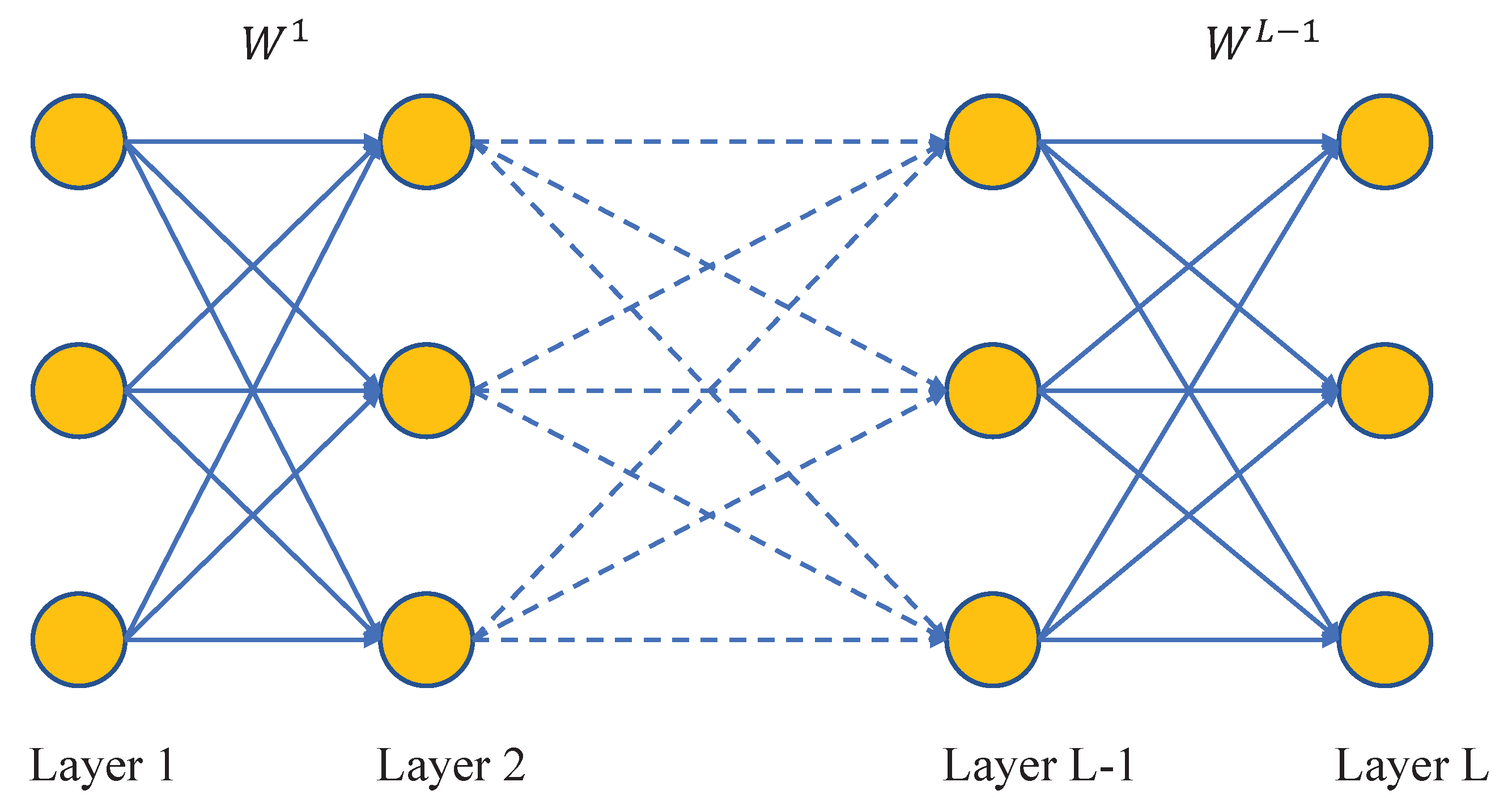
A BPNN is a type of feedforward neural network (FNN). The simple architecture of a BPNN is shown in Figure 1, where the neurons in the same layer of the BPNN are only connected with adjacent layers’ neurons; there are no connections among neurons in the same layer. The BPNN contains three types of layers: the input layer, hidden layers, and output layer. Input layer inputs data into the neural network. Output layer outputs the neural network’s computational results. The hidden layers are the layers between the input layer and output layer. The values of connections between different layers are weights denoted by w i where i denotes i-th layer. All the knowledge that the neural network has learned is stored in the weights.
The goal of training a BPNN is to determine a set of suitable W so that the network can obtain the correct output when test data is input into it by training on the train dataset. Suppose there is a training set x 1 , y 1 , ( x 2 , y 2 ) , , ( x n , y n ) , which contains n tuples. Each tuple contains input data x i and target label y i . To train a BPNN, the first step is forward computing, which can be computed as
z l + 1 = W l a l , a l + 1 = f ( z l + 1 ) ,
where z l is the l-th layer’s input vector, a l is the l-th layer’s output vector, and f ( · ) is an active function. In this paper, we chose the rectified linear unit as our active function, which is defined as
f x = x , i f x > = 0 , 0 , e l s e .
After forward computing, the BP networks need to update the network through the losses that were calculated from the target labels so that the network can determine the suitable W, where W is a set of W 1 , , W L and L is the number of layers. One of the most commonly used update methods is the gradient descent method with BP. The BP process starts by defining a loss function, Loss. The loss function measures the distance between the outputs of the BP network and the true targets. The mean-square error (MSE) is a common loss function for prediction. It is defined as Equation (3):
L o s s = 1 2 n L i = 1 n L y i L ( x ) a i L 2 ,
where y i L is the i-th output of the output layer, a i L is the i-th target label of output layer, and n L is the total number of outputs in the output layer. 1 2 is for better computing the derivative of loss. Because a i L is computed by W, loss function L o s s is the function of weight W.
To use the gradient descent method to determine the optimal W, we need to compute W which is defined as
W = L o s s W ,
and update W using
W = W α W ,
where α is the learning rate, which controls the learning step during each update. We define an error term in the i-th neuron l-th layer as δ i l = L z i l for better computation of gradient W in each layer.
In the output layer, we can compute the gradient of w i j L directly by combining Equation (3) and using the chain rule:
L o s s w L = L o s s z L z L w L = δ L ( a L 1 ) T .
Then, we compute the other layers’ error terms using back propagation:
δ l = L o s s z l = L o s s z l + 1 z l + 1 z l = f ˙ ( z l ) ( ( w l ) T δ j l + 1 ) .
Then, we compute the remaining layers’ weight gradients from back to front in matrix form as
W l = δ l + 1 ( a l ) T .
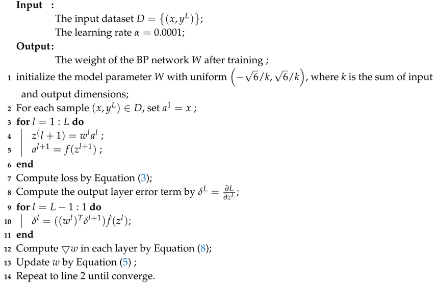
Thus, the learning process of the BPNN can be presented as Algorithm 1.
Algorithm 1: The BP network update process with gradient decent.
Energies 12 01433 i001

2.2. RNN

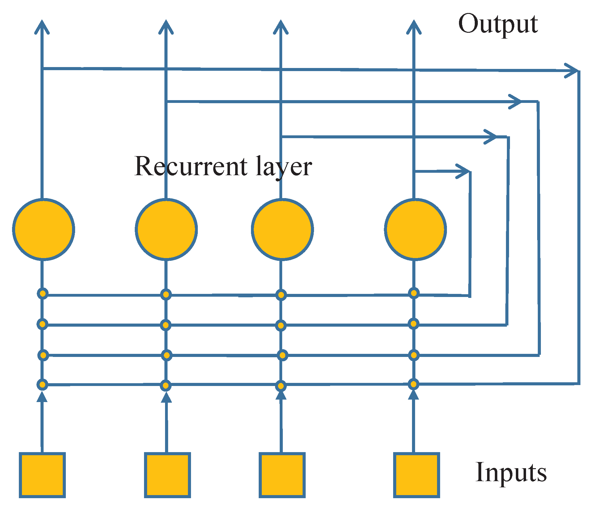
STLF is a type of prediction based on the previous time. It is based on the history load information forecasting the next time load value. We can consider it as a sequential problem. Among all types of neural networks, the RNN is good at solving sequential problems. An RNN contains recurrent connections. A simple architecture of an RNN is shown in Figure 2. It contains an input layer, recurrent layer, and output layer. The difference between an RNN and BPNN is that an RNN has connections among the same recurrent layer’s neurons.
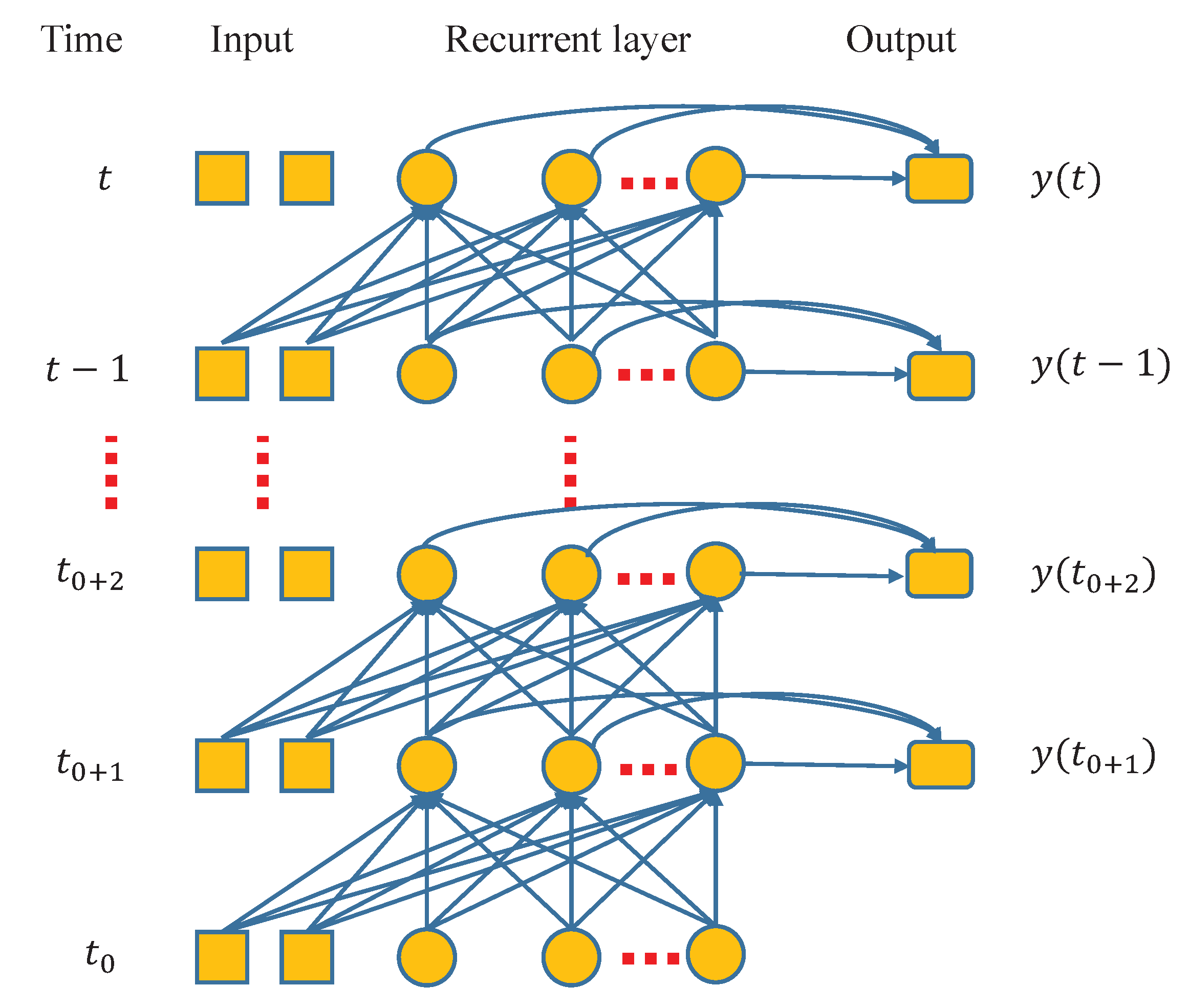
For a better understanding of the computation of an RNN, we can unroll the RNN on the time dimension as shown in Figure 3. In the unrolled RNN, the neurons in the hidden layer at each time step t can be considered as one layer of an FNN. If the time step is T, then the unrolled RNN has T hidden layers. Based on the unrolled network, we can train the RNN using backpropagation through time (BPTT) [46], specifically epoch-wise BPTT, using the following steps:
  • Forward computing: the output of network at time t can be computed as the following equation:
    s ( t + 1 ) = x ( t ) + w y ( t ) , y ( t + 1 ) = f ( s ( t + 1 ) ) .
  • Define the loss as
    E ( t , t ) t o t a l = τ = t + 1 t E ( τ ) , τ t 0 + 1 , t ,
    where E ( t ) = 1 2 d ( t ) y ( t ) 2 is the error at time t . At each time step, d ( t ) represents the target label and y ( t ) is the output of the network at time t .
  • Compute gradient w of w as follows:
    w = E ( t 0 , t 1 ) t o t a l w = τ = t 0 + 1 t E ( t 0 , t 1 ) t o t a l w ( τ ) .
    Combine with the chain rule and define e ( τ ) = E ( τ ) y ( τ ) , which can be written as
    E ( t 0 , t 1 ) t o t a l w ( τ ) = δ ( τ ) ( y ( τ 1 ) ) T ,
    where
    δ k ( τ ) = f ( ˙ s ( τ ) ) e ( τ ) , w h e n τ = t , f ( ˙ s ( τ ) ) ( e ( τ ) + w T δ ( τ + 1 ) ) , w h e n t 0 < τ < t .
    Hence, the gradients of weights can be computed as
    w = δ ( τ ) ( y ( τ 1 ) ) T .
  • Then, update the weights in the RNN using Equation (5) until the network converges.

2.3. LSTM

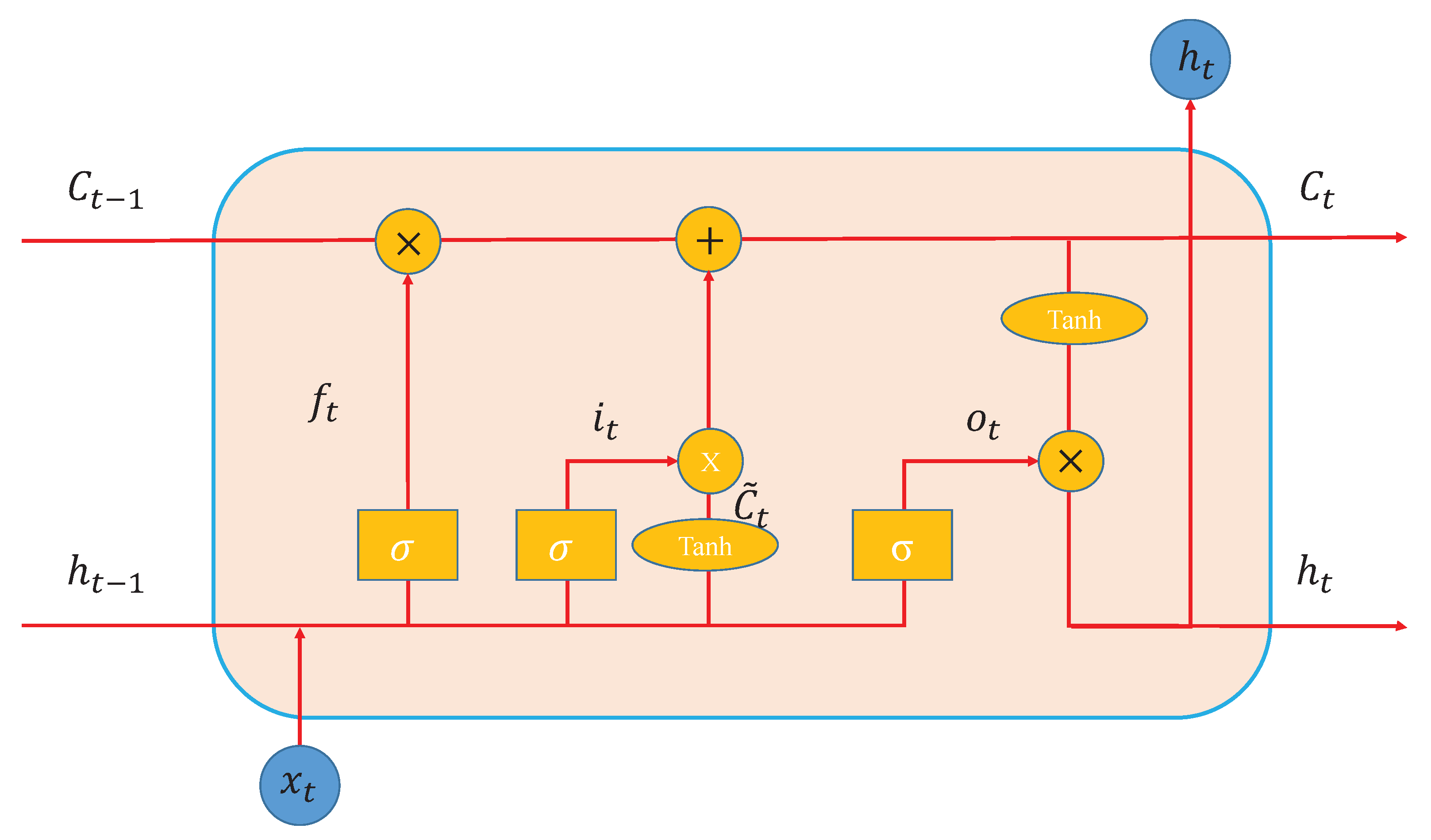
LSTM is a type of RNN, but it has a more complicated architecture. A common LSTM network consists of many LSTM blocks, which are called memory cells. An LSTM cell stores the input for some period of time. The flow of information into and out of the cell was determined by the values in the cell and regulated by the three gates. A classical cell architecture is shown in Figure 4. The cell receives input x t at time t, output h t 1 and state vector C t 1 at time t 1 . There are three gates in the cell to control the computation of the cell: the input gate, output gate and forget gate. The input gate selectively records new information into the cell state. The output gate determines which information is worth outputting. The forget gate selectively forgets some information and retains much more valuable information. The forward pass of an LSTM unit with a forget gate can be computed as following equations
f t = σ g ( W f x t + U f h t 1 ) , i t = σ g ( W i x t + U i h t 1 ) , o t = σ g ( W o x t + U o h t 1 ) , c t = f t · c t 1 + i t · σ c ( W c x t + U c h t 1 ) , h t = o t · σ h ( c t ) ,
where x t is the input vector to the cell. W R h × d and U R h × h are the weight matrices and bias vector parameters, where h and d refer to the number of input features and number of hidden units. f t , i i and O t are the forget gate, input gate and output gate’s output, respectively. h t is the hidden state vector, which is also called the output vector. c t is the cell state vector. σ g , σ c and σ h are activation functions, where σ g is the sigmoid function, σ c is the hyperbolic tangent function and σ h is the hyperbolic tangent.
To update the parameters of LSTM, a common way is using epoch-wise BPTT algoritm as the same with RNN, the detail can be found in [47].

2.4. Gate-RNN

As we can see, BPNN is an FNN. If BPNNs are used to predict load, they will weaken the relationships in the time dimension. Regarding RNN and LSTM, they are good at capturing temporal features. However, RNN can only memory history information through the weights among neurons, which is much is too simple to handle the input information and memory information. By contrast, during an experiment, we found that LSTM was too complicated to train stably. Thus, we propose an RNN cell that can control the computation of input information and memory information, converges well in the training process, and has excellent results in ultra STLF.
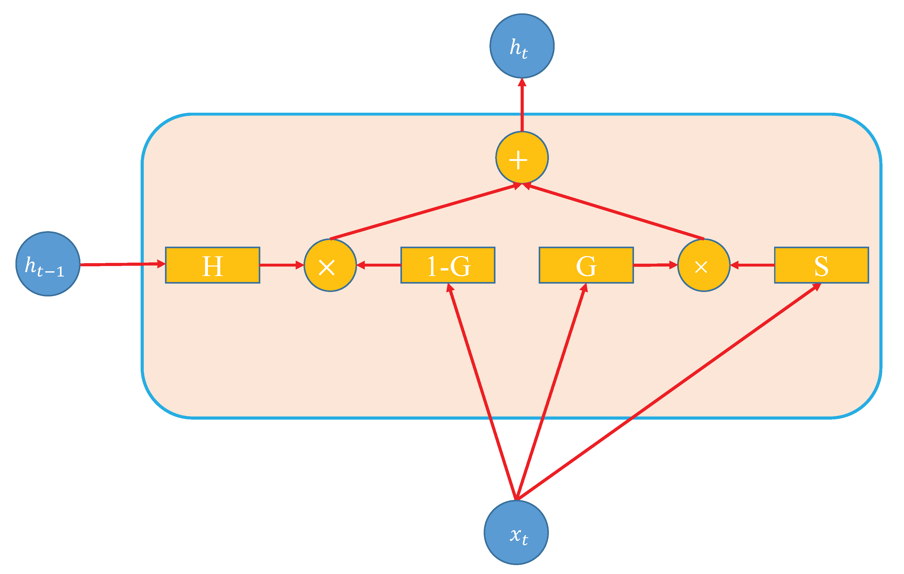
Figure 5 shows the cell architecture of our gate-RNN. At time t, the input vector of the cell is x t and the history information is output h t 1 at time t 1 . When input vector x t is input into the cell, it is divided into three branches: two branches for computing two gates’ values that are 1 G and G, and one for computing the cell’s state that is S. Gate G controls the effect of the cell state on the output and gate 1 G controls the effect of history information on the output. The output of the cell h t combines the output of both gates. We use the + operator as our combination approach, and it adds the values of both gates at the same position.
The computation of the cell is as follows:
g t = W g x t , s t = W s x t , h ˜ t = W h h t 1 , h t = g t · s t + h ˜ t · ( 1 g t ) ,
as for LSTM, W R h × d denotes the weight matrices parameters. Many gate-RNN cells are combined to obtain a layer and then a neural network. To update the gate-RNN, we compute the gradient of the weight at each time step. We also define an error term at the t-th time step (same as the l-th layer) as δ t = L o s s h t to better compute the gradient of W in each layer. In the t-th time step, we can compute the gradients of W g , W s , W h directly by combining Equation (3) and using the chain rule, as follows:
W g = L o s s W g = L o s s h t · h t g t · g t W g = δ t · ( ( s t h ˜ t ) · ( x t ) ) T ,
W s = L o s s W s = L o s s h t · h t s t · s t W s = δ t · ( g t · ( x t ) ) T ,
W h = L o s s W h = L o s s h · h t h ˜ t · h ˜ t W h = δ t · ( ( 1 g t ) · ( h t 1 ) ) T .
Then, we update the entire network using Algorithm 2.
Algorithm 2: The update process of gate-RNN.
   Input  :
       The input dataset D = ( x , y L ) ;
       The learning rate α = 0.0001 ;
   Output:
       The weight of the gate-RNN network W after training;
1 
initialize the model parameter W with uniform 6 / k , 6 / k ;
2 
For each sample ( x , y L ) D , set a 1 = x ;
3 
Do forward computing by using Equation (16);
4 
Compute loss by Equation (3);
5 
Compute the last time step T error term by δ g T = L o s s g T , δ h T = L o s s h T , δ s T = L s T ;
6 
Compute gradients of W s , W h , W g , by using Equation (17)–(19);
7 
Update W by Equation (5);
8 
Repeat to line 2 until converge.

3. Experiments Results and Discussion

3.1. Experiment Data Processing and Experiment Settings

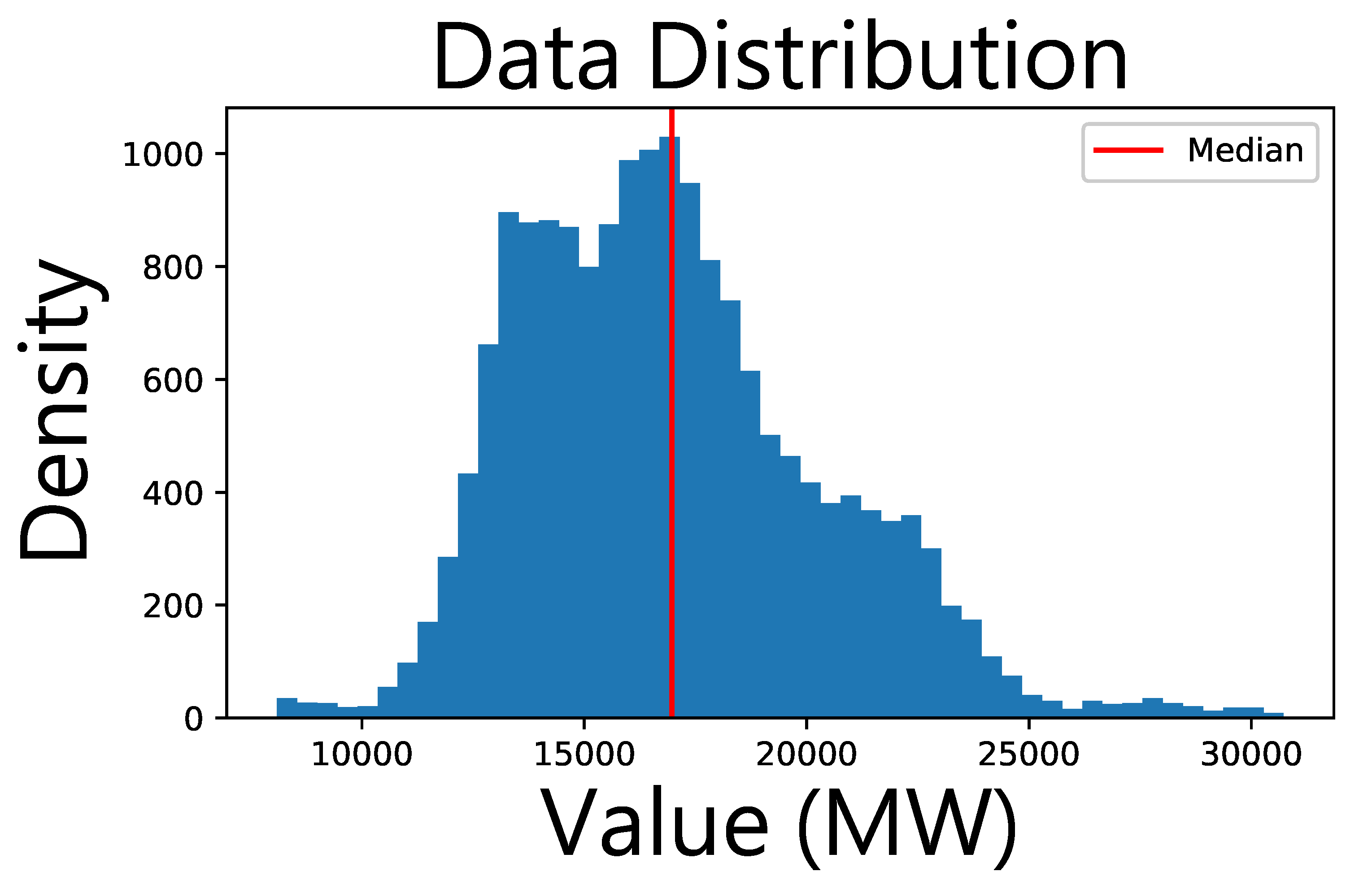
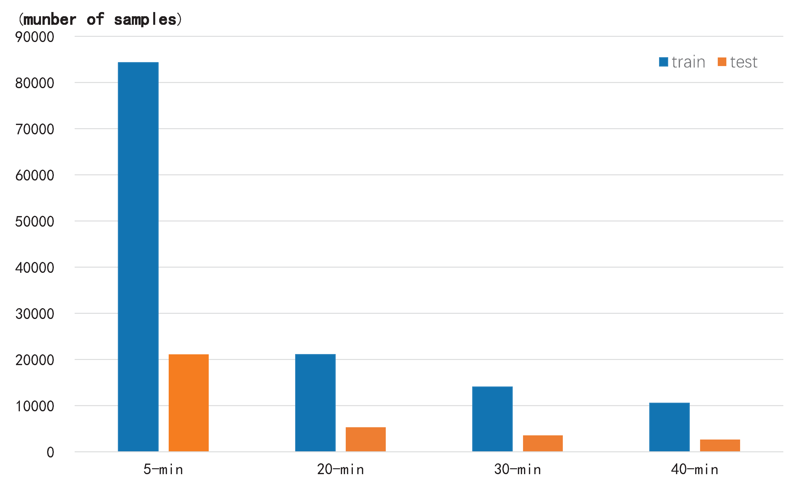
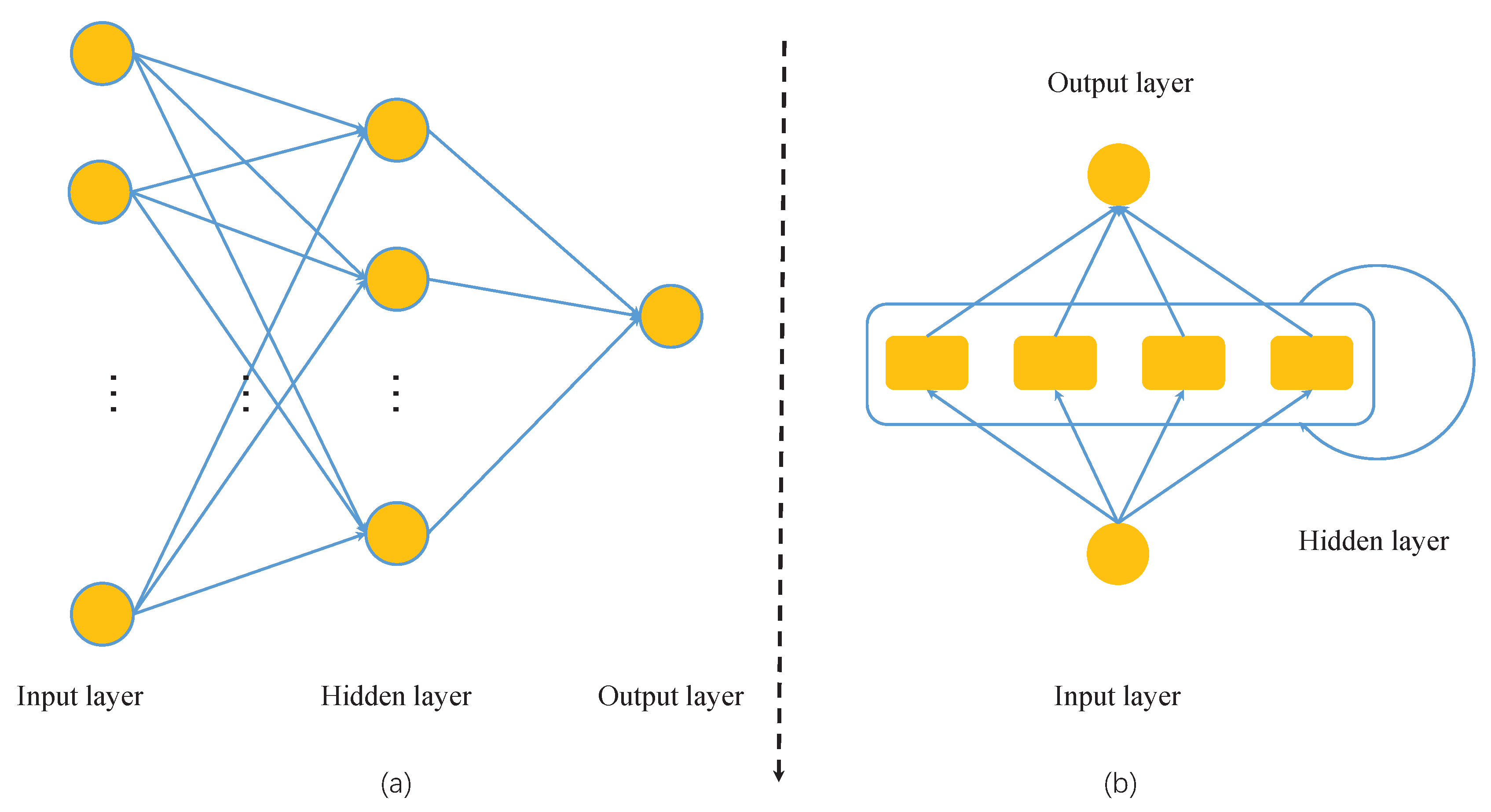
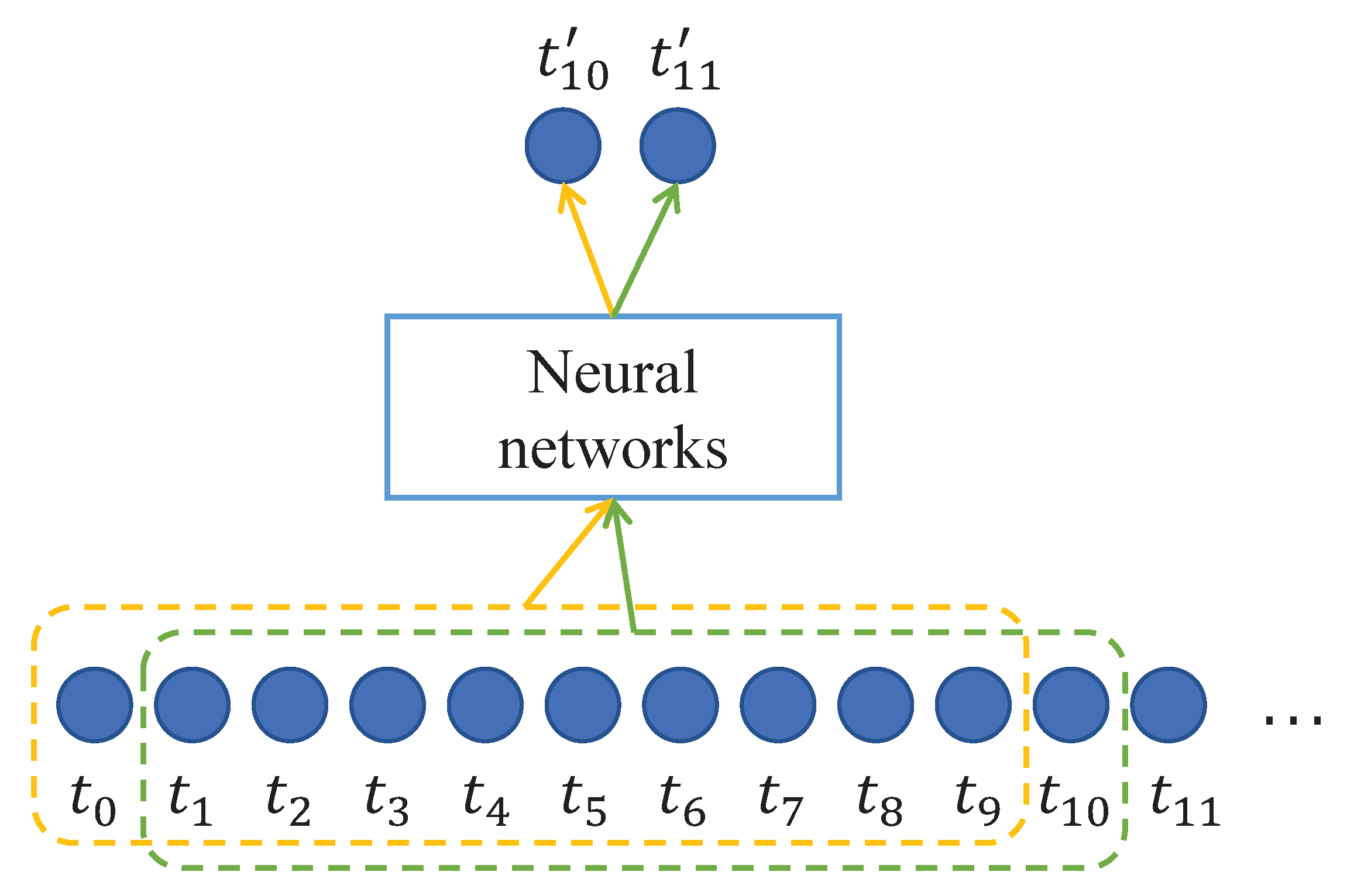
Our dataset contained an entire year’s electrical load of the 2016 Electric Power Company in Sichuan Province, China. The data values distribution is shown in Figure 6. The average, variance, standard deviation and coefficient of variation are 16,965.71, 11,692,942.24, 3419.49 and 4.96, respectively. To avoid overlap between the training data and test data, all the data were sorted by time, and the first three-quarters of the total data was chosen as our training data and the remainder as our test data. It means that we used nine months’ load values as the train date, the rest of the three months’ load values as test sets. Because, for training neural networks, it is suggested to use raw data, we don’t use any regularization or pay special attention to the special days in the whole years such as holidays and Chinese New Year day. The original data recorded electrical load with a 1 min interval. According to the data processing method in [7], the data were sampled for different time scales. For a better analysis of neural network performance, the data were sampled for 5-min, 20-min, 30-min, and 40-min time scales after dividing the training data and test data into different time scales. The data size of different time scales’ train dataset and test dataset are shown in Table 1. It can be visualized as in Figure 7. As we can see, with the time scale become larger, the size of dataset become smaller. Because of sampling by different time scales, the data have been divided into different sizes. Regarding training the BPNN, the inputs of the neural networks were the last 10 samples and the output was the prediction value of the 11th moment load value. For the RNN series methods, the input was the previous nine load values and the current load value, and the output was the next time predicted load value. All the input values are the nearest ten values and ordered in time; this is the same way as mentioned in [35,43]. The complete structures of ANNs are shown in Figure 8. After predicting the eleventh load value, the second value to the eleventh value is chosen to predict the twelfth value. We iterate this procedure until finishing the prediction of the last value. The prediction mechanism of the neural network is shown in Figure 9.
In the experiment, the following criteria were used to evaluate all the mentioned methods: the root mean square error (RMSE), mean absolute error (MAE) and mean absolute prercentage error (MAPE), which are widely used in STLF [1,7,17]. They are calculated as follows:
R M S E = 1 N i = 1 N ( x i x i ˙ ) 2 ,
M A E = 1 N i = 1 N x i x i ˙ ,
M A P E = 1 N i = 1 N x i x i ˙ x i × 100 % ,
where x i is the actual load value, x i ˙ is the predicted load value, N is the number of test samples. These criteria represent three types of deviation between the forecast and actual values: the smaller the criteria, the higher the forecasting accuracy. MAE is the basic metric for STLF, RMSE is sensitive to the regression point with large deviation, and MAPE considers both the error and the ratio which are between the predicted value and true value.
In order to balance performance and accuracy, we tried several trials to decide the size of all the neural networks in a 30-min time scale data set, the trails’ results on 30-min test set are shown in Table 2. The number after the methods is the number of neurons. We have tried a three-layer BPNN architecture, and the results show it can forecast the load values well when the number of hidden neurons is 64. More or less hidden neurons will cause a decrease in performance. It means that a three-layer BPNN with 64 hidden neurons is a good choice for this load forecast task. Therefore, we have not added more layers into BPNN. The same as with BPNN, from the results, we can see that one recurrent layer with four neurons is a good choice for this load forecast task. The specific configuration of the mentioned neuron networks for STLF was as follows: The BPNN contained three layers. Specifically, the first layer was the input layer, which contained 10 neurons, and each input was a sampled load value; the second layer was a hidden layer whose size was 64; and the last layer was the output layer, which only contained one neuron, which represented the predicted value. The RNN, LSTM, and gate-RNN input layers contained one neuron, which was input into a 4-neuron RNN, LSTM, or gate-RNN cell, and the output was the same as that of the BPNN. The RNN cell calculated the value of the last 10 moments to predict the value of the next moment. All the networks in this paper were implemented using the Keras framework. The loss function of these methods was Equation (22). The optimizer of the neural networks was RMSProp and its parameters were set as Keras default parameters except for the learning rate. During the training process, the learning rate of epoch 1 to 5 was 0.01 and the remaining epoches learning rate was 5 × 10 5 . The total number of epoch was 55 and the value of weight decay is 5 × 10 5 .

3.2. Comparison of the Models with the Baseline Method

To evaluate the effectiveness of the neural network methods mentioned in the section above, several most commonly used traditional methods were chosen as the baseline methods. They are SVR [22], decision tree (DT) [9], autoregressive integrated moving average model (ARIMA) [48], and one random forest (RF) proposed in [49]. SVR is one of the most popular methods that is widely used to forecast short-term load. DT, ARIMA and RF introduced in [49] are useful methods. All these methods have been used in STLF in different time scales, 5-min, 20-min, 30-min and 40-min time scale [9,48,49]. The results of all the methods test on the test set of three months are shown in Table 3, Table 4, Table 5 and Table 6. From these tables, we can see that among the eight methods, the neural network methods achieved better comprehensive performance compared with other traditional methods in all different time scales, except LSTM. In a smaller time scale, specifically in 5-min and 20-min, gate-RNN achieved better performance than any other methods. ARIMA achieved the best performance among all the traditional methods. On a larger time scale, 30-min and 40-min, BP achieved better comprehensive performance than any other methods. Meanwhile, DT achieved the best performance among all traditional methods. It has shown that the performance of methods is influenced by the time scale.
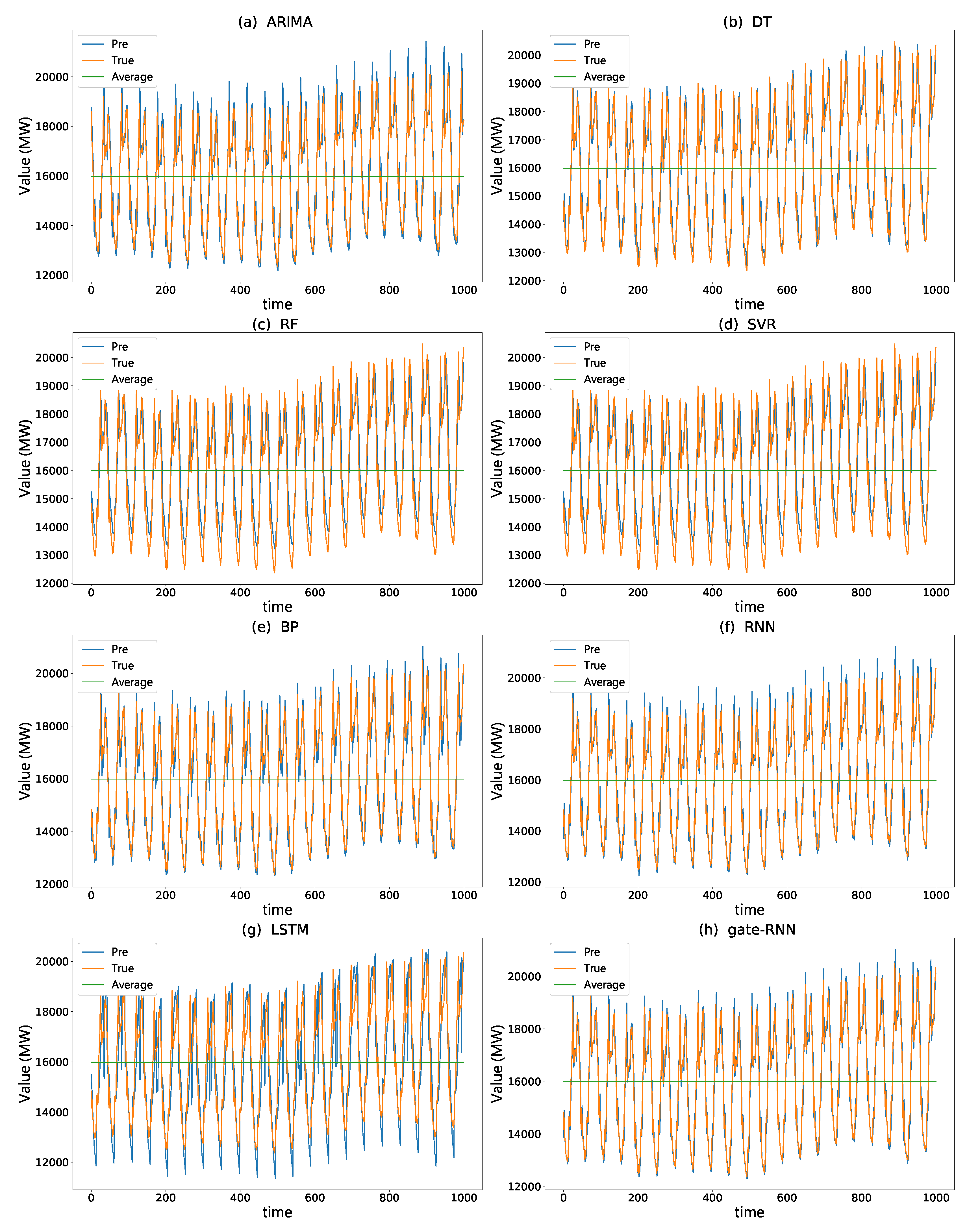
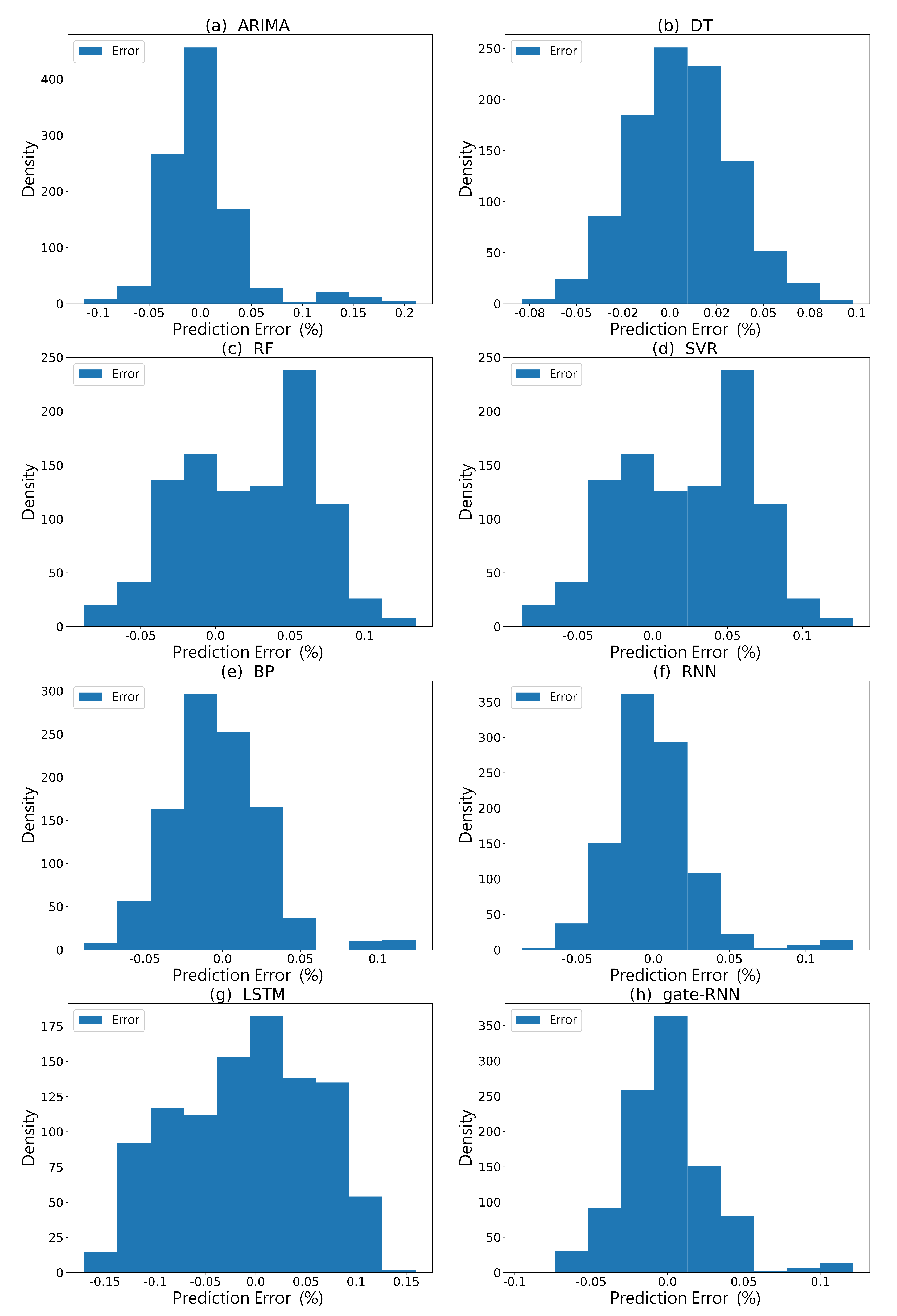
To clearly illustrate the forecast value, from the test set of three months, we chose 1000 time scales’ actual and predicted electric load values obtained by the eight methods to draw a figure on a 30-min time scale, which is shown in Figure 10. The orange line stands for real load values, the blue line stands for prediction values and the green line stands for the average value of real load values. Furthermore, 1000-time scales are nearly one month, from Figure 10, we can see the blue line is far away from the green line and close to the orange line. All of the methods’ prediction values are much closer to the real values; this means that the prediction values have no relations to the average value for some months and even one year. Specifically, it can be seen that the predicted values obtained by the LSTM method have the maximum error for the original data compared with the other seven methods; particularly, the other three types of neural network methods. This is because the structure of LSTM is much more complicated than the other three types of neural networks. To achieve equivalent performance, LSTM needs much more data than BP, RNN, and gate-RNN. It is difficult to train an LSTM for STLF using only one year of load data. Additionally, we plot the error distribution of each model in 30-min time scale, which is shown in Figure 11. RNN and gate-RNN are more accurate and effective, while the errors of other methods are scattered in a wider distribution space.

3.3. Performance Analysis of the Neural Networks

In this section, we analyze the performance of four neural network methods which include the training process of different neural networks and the performance of the neural networks. To better compare these methods, we used four time scales to process the data: 5 min, 20 min, 30 min, and 40 min.

3.3.1. Training Process Analysis for the Neural Networks

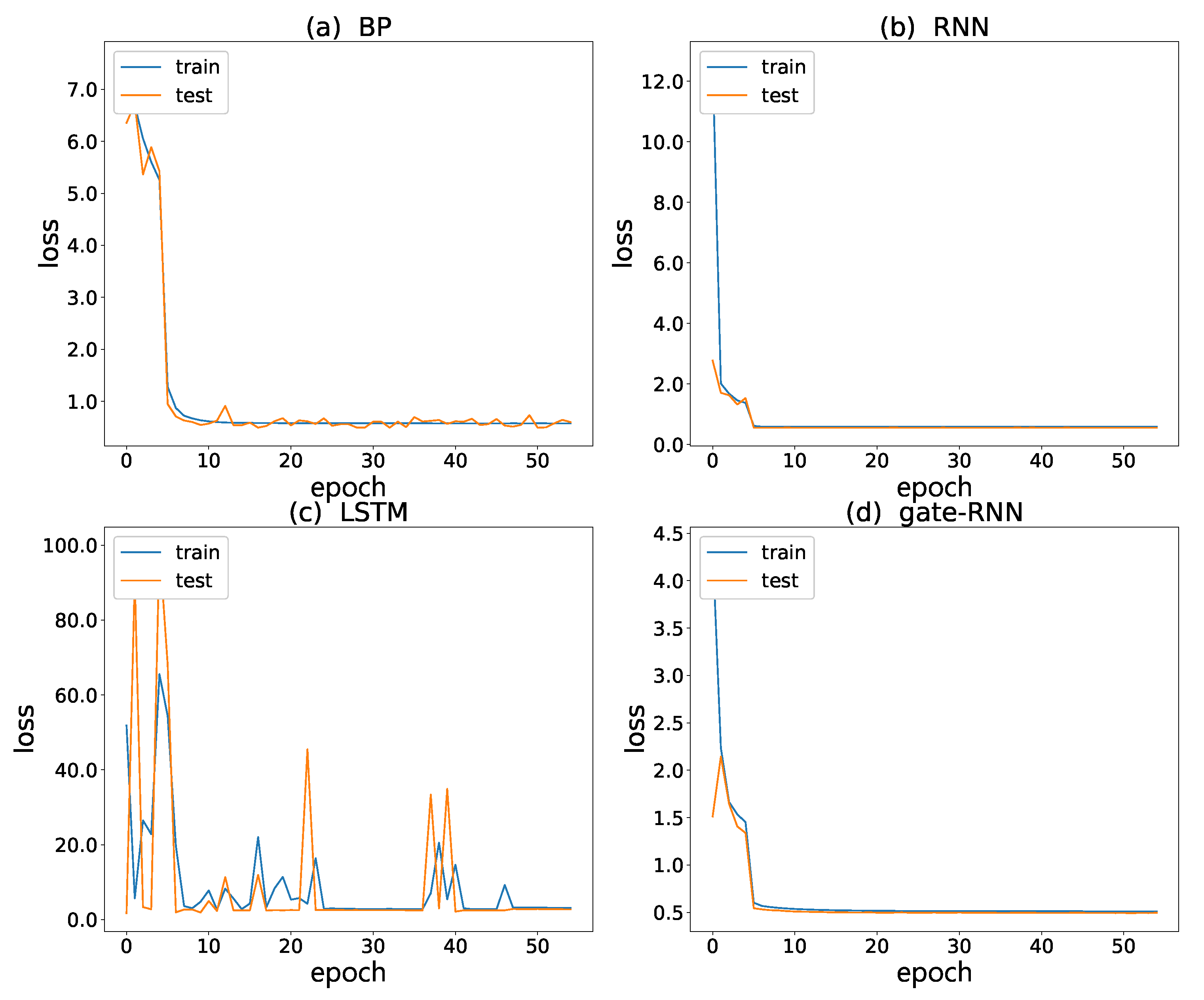
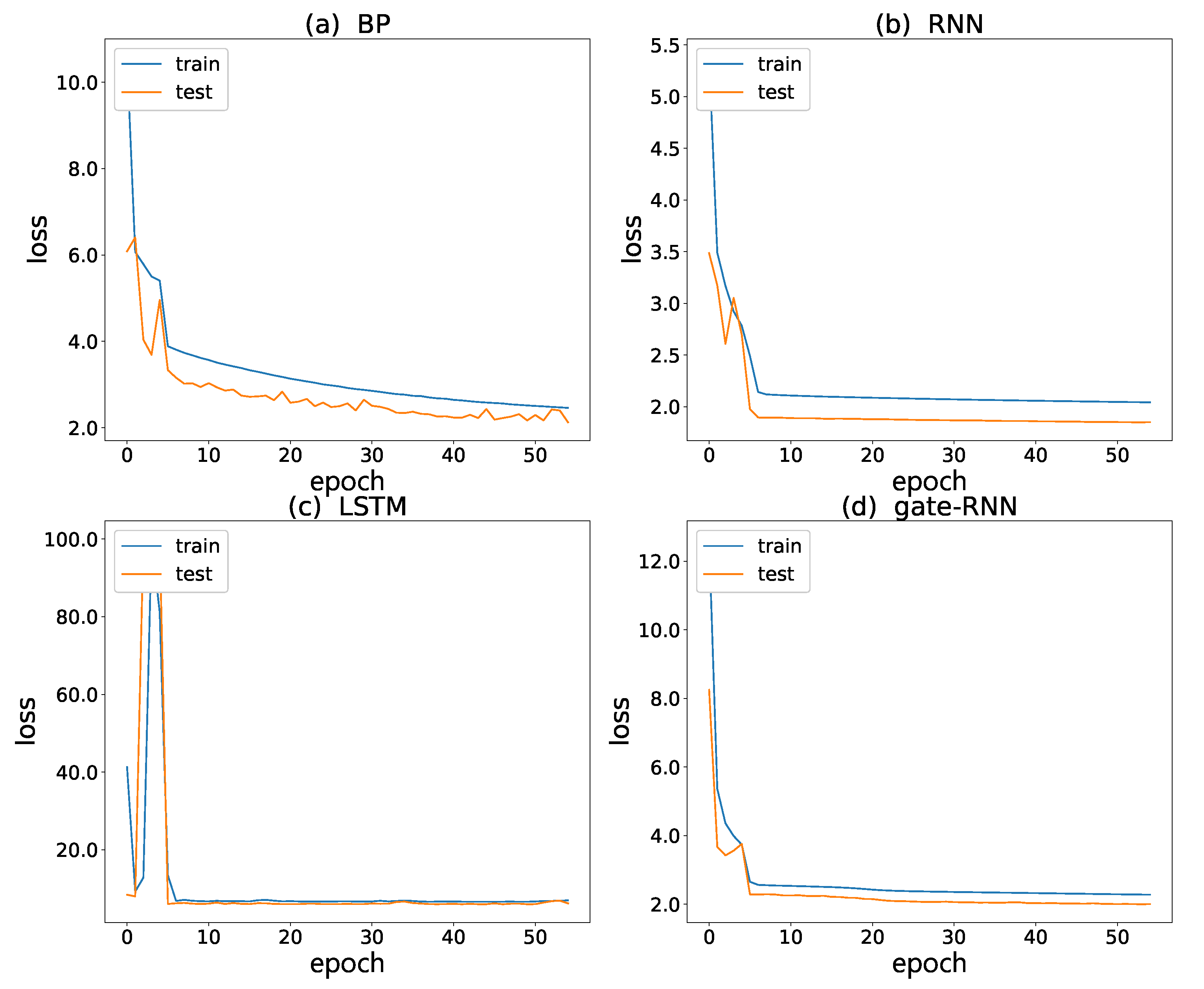
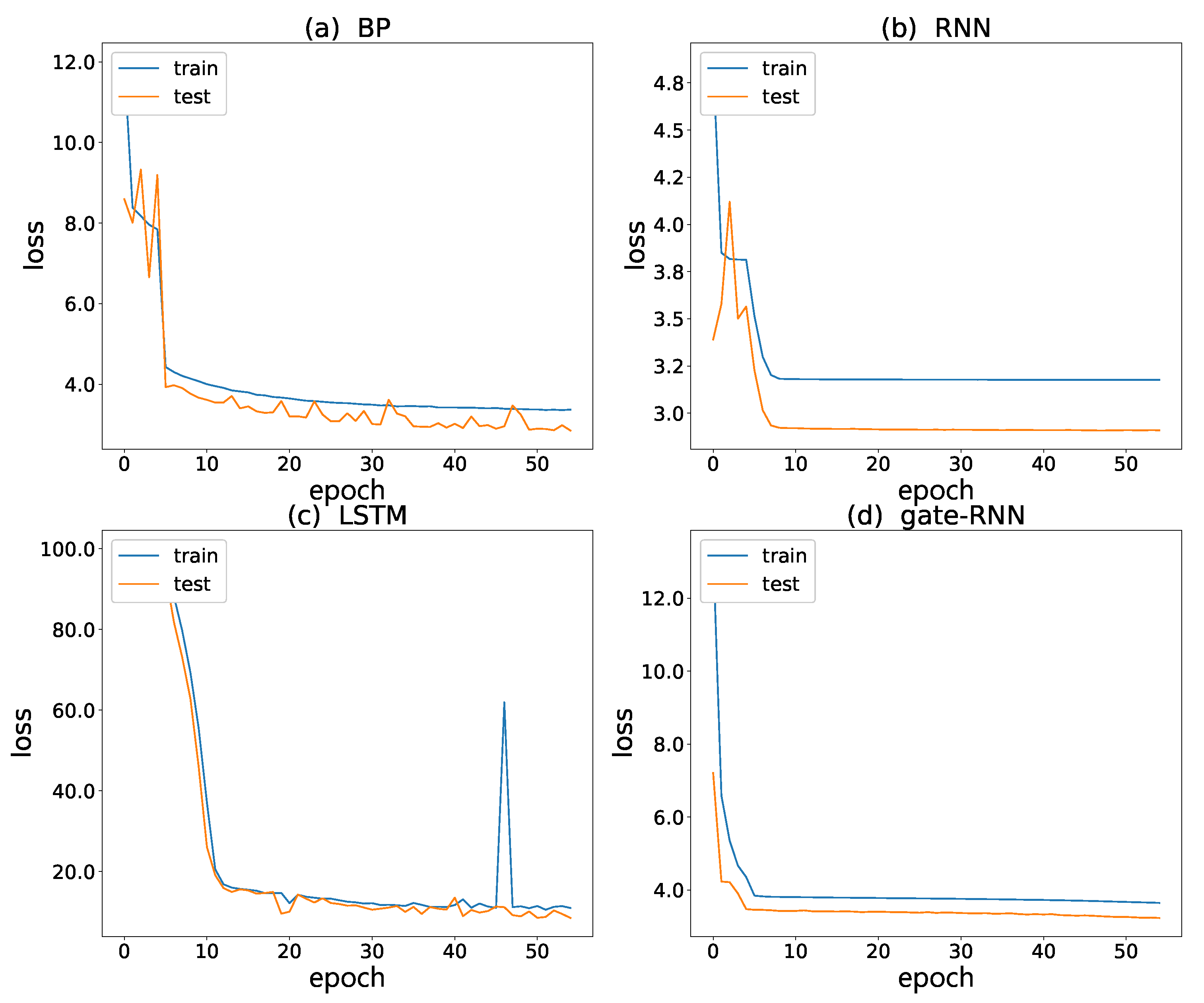
To assess whether the neural networks were trained and learned the distribution of data, a direct approach is to assess whether the train loss and test loss converged. From Figure 12, Figure 13, Figure 14 and Figure 15, we can see that the RNN and gate-RNN train loss and test loss converged well for all time scales; LSTM had large fluctuations and BP had slight fluctuations. For the 5-min time scale, even though LSTM had a large fluctuation, all the methods achieved a small train loss and test loss, and the trends of the train loss and test loss were the same. This means that all the methods learned the distribution of train data and achieved good performance on the test set. When the time scale was larger than 5 min, even though the trends of the train loss and test loss were the same, the convergence values of the train loss and test loss were different, and the losses increased as the time scale increased. This means that, as the time scale increased, the performance of the neural network became worse.
From Figure 12, Figure 13, Figure 14 and Figure 15, we also can find that our proposed method converged after training in approximately five epochs, which was faster than any of the other methods. BP converged in approximately ten epochs and RNN converged in approximately seven epochs. This means that our proposed method had significant power to forecast ultra short-term load. We believe that it benefits from the suitable gate mechanism. The RNN method has no gate mechanism; it cannot choose the memory information, but the LSTM method was too complicated to train on the data.

3.3.2. Examination of All the Neural Networks

After analyzing the train loss and test loss, we analyzed the criteria for each method for different time scales. The results for the four neural networks are shown in Table 7, Table 8 and Table 9. Table 7, Table 8 and Table 9 which present the RMSE, MAPE, and MAE, respectively, for four time scales. Table 7 shows that gate-RNN achieved the best performance for the 5-min and 20-min time scales; RNN achieved the best performance for the 30-min time scale; and BP achieved the best performance for the 40-min time scale. The results in Table 8 and Table 9 show the same performance as Table 7 where gate-RNN achieved the best performance for the 5-min and 20-min time scales; RNN achieved the best performance for the 30-min time scale; and BP achieved the best performance for the 40-min time scale. Overall, gate-RNN achieved good results among all the four methods. This proves that our proposed method is better at forecasting ultra short-term load again.
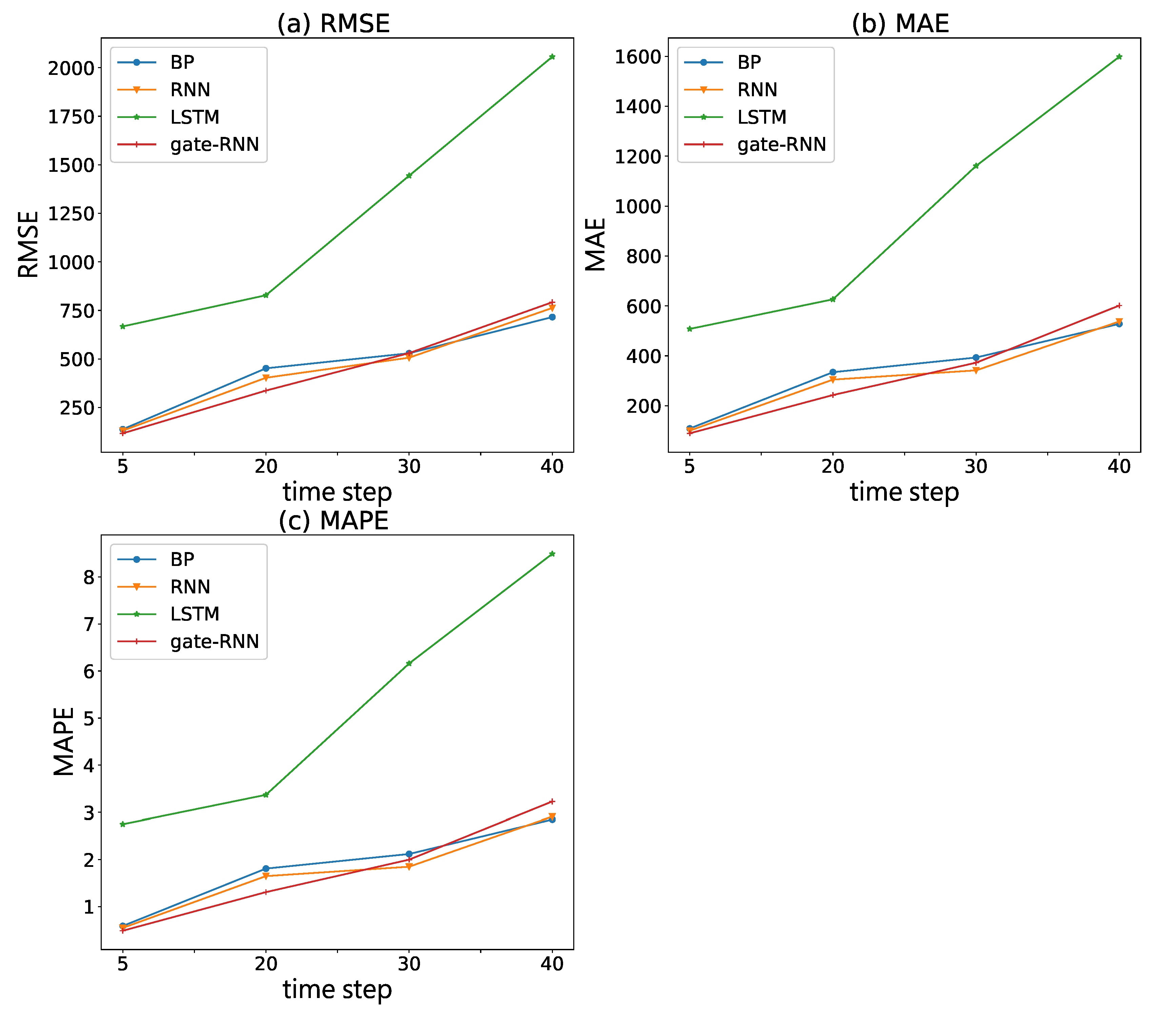
Further visualization results are shown in Figure 16. We can see it intuitively that the performance of all the methods became worse as the time scale increased. Overall, all the methods had a similar trend: they began at a relatively small value and ended with a large value. Figure 16 also shows that our method achieved the best results for the criteria for small time scales, but, as the time scales increased, our method’s performance became slightly worse. Overall, the performance of LSTM for all criteria for different time scales was worse, and the values for the criteria were far from those of the other neural network methods.
We believe that this scenario was caused by the following main points. First, we consider the reason that the data is time scale. The larger the time scale, the more likely that unpredictable states will affect the load value, such as sudden weather changes and holidays. Even though the neural networks could predict the trend of the load, the values of the load would have a large turbulence. Second, we consider the neural networks’ features. As we know, the complexity of the structures increases gradually in the following order: BP, RNN, gate-RNN, and LSTM. The more complex the architecture of a neural network, the more difficult it is to train it, and the more data are needed to train it. After we process the data into different time scales, the data size changes according to the time scale. For example, the number of total data items is T t o t a l recorded every 1 min, so, when our time scale is 5 min, the data items become T 5 m i n , which is 1 5 of the total items, that is, five times smaller than T t o t a l . All of the time scales can be represented by T t o t a l = 5 × T 5 m i n = 20 × T 20 m i n = 30 × T 30 m i n = 40 × T 40 m i n . Thus, when using these different time scales to process data to train the networks, the actual data size decreased with the time scale, and then the performance became worse with an increase in the time scale.

4. Conclusions

The aim of our work was to explore the performance of different types of neural networks in the STLF, and, based on the insufficiency of current neural networks, we proposed a new neural network architecture called the gate-RNN. Our proposed method is extremely suitable for handling ultra STLF. From the experimental results, we found that neural networks have the STLF ability. They can achieve better performance than the tranditional methods. However, the more complex the neural network’s architecture, the more data are needed to train the neural network. Considering that different neural networks have different characteristics, for our dataset, the gate-RNN achieved the highest score overall. For a large time scale, the BP achieved better performance than RNNs.
In future research, we plan to improve our work in two aspects. First, we will extend our data to multivariate data. Collecting more electrical load data and adding more relevant factors can influence load forecasting, for example, weather and some breaking news information. Second, based on the gate-RNN, to train the neural network more efficiently, we plan to design a loss function that can reflect the forecasting value online.

Author Contributions

Data curation, L.Y.; Formal analysis, L.Y.; Funding acquisition, H.Y.; Methodology, L.Y.; Supervision, H.Y.; Writing—original draft, L.Y.; Writing—review and editing, L.Y.

Funding

This research was funded by the National Natural Science Foundation of China Grant No. 51477105.

Acknowledgments

We thank those who provided constructive comments and feedback to help improve this paper.

Conflicts of Interest

The authors declare no conflict of interest.

Abbreviations

The following abbreviations are used in this manuscript:
STLFShort-term load forecasting
ANNartificial neural network
SVMSupport vector machine
SVRSupport vector regression
BPNNBack propagation neural network
RNNRecurrent neural network
LSTMLong-short-term memory
gate-RNNGate-recurrent neural network
MAEMean absolute error
RMSERoot mean square error
MAPEMean absolute percentage error
DTDecision tree
ARIMAAutoregressive integrated moving average model
RFRandom forest

References

  1. Bunn, D.W. Forecasting loads and prices in competitive power markets. Proc. IEEE 2000, 88, 163–169. [Google Scholar] [CrossRef]
  2. Senjyu, T.; Mandal, P.; Uezato, K.; Funabashi, T. Next Day Load Curve Forecasting Using Hybrid Correction Method. IEEE Trans. Power Syst. 2005, 20, 102–109. [Google Scholar] [CrossRef]
  3. Nataraja, C.; Gorawar, M.; Shilpa, G.; Harsha, J.S. Short term load forecasting using time series analysis: A case study for Karnataka, India. Int. J. Eng. Sci. Innov. Technol. 2012, 1, 45–53. [Google Scholar]
  4. Goia, A.; May, C.; Fusai, G. Functional clustering and linear regression for peak load forecasting. Int. J. Forecast. 2010, 26, 700–711. [Google Scholar] [CrossRef]
  5. Trudnowski, D.J.; Mcreynolds, W.L.; Johnson, J.M. Real-time very short-term load prediction for power-system automatic generation control. IEEE Trans. Control Syst. Technol. 2001, 9, 254–260. [Google Scholar] [CrossRef]
  6. Wang, H.; Schulz, N.N. Using AMR data for load estimation for distribution system analysis. Electr. Power Syst. Res. 2006, 76, 336–342. [Google Scholar] [CrossRef]
  7. Jiang, H.; Zhang, Y.; Muljadi, E.; Zhang, J.J.; Gao, D.W. A Short-Term and High-Resolution Distribution System Load Forecasting Approach Using Support Vector Regression with Hybrid Parameters Optimization. IEEE Trans. Smart Grid 2017, 9, 3341–3350. [Google Scholar] [CrossRef]
  8. Capizzi, G.; Sciuto, G.L.; Napoli, C.; Tramontana, E. Advanced and adaptive dispatch for smart grids by means of predictive models. IEEE Trans. Smart Grid 2018, 9, 6684–6691. [Google Scholar] [CrossRef]
  9. Hambali, A.O.J.; Akinyemi, M.; JYusuf, N. Electric Power Load Forecast Using Decision Tree Algorithms. Comput. Inf. Syst. Dev. Inform. Allied Res. J. 2016, 4, 29–42. [Google Scholar]
  10. Bonanno, F.; Capizzi, G.; Sciuto, G.L. A neuro wavelet-based approach for short-term load forecasting in integrated generation systems. In Proceedings of the 2013 International Conference on Clean Electrical Power (ICCEP), Alghero, Italy, 11–13 June 2013; pp. 772–776. [Google Scholar]
  11. Tian, C.; Ma, J.; Zhang, C.; Zhan, P. A Deep Neural Network Model for Short-Term Load Forecast Based on Long Short-Term Memory Network and Convolutional Neural Network. Energies 2018, 11, 3493. [Google Scholar] [CrossRef]
  12. Tian, C.; Hao, Y. A novel nonlinear combined forecasting system for short-term load forecasting. Energies 2018, 11, 712. [Google Scholar] [CrossRef]
  13. Zhang, X. Short-term load forecasting for electric bus charging stations based on fuzzy clustering and least squares support vector machine optimized by wolf pack algorithm. Energies 2018, 11, 1449. [Google Scholar] [CrossRef]
  14. Merkel, G.; Povinelli, R.; Brown, R. Short-term load forecasting of natural gas with deep neural network regression. Energies 2018, 11, 2008. [Google Scholar] [CrossRef]
  15. Li, G.; Li, B.-J.; Yu, X.-G.; Cheng, C.-T. Echo state network with bayesian regularization for forecasting short-term power production of small hydropower plants. Energies 2015, 11, 12228–12241. [Google Scholar] [CrossRef]
  16. Hu, C.; Luo, S.; Li, Z.; Wang, X.; Sun, L. Energy coordinative optimization of wind-storage-load microgrids based on short-term prediction. Energies 2015, 8, 1505–1528. [Google Scholar] [CrossRef]
  17. Fan, S.; Hyndman, R.J. Short-term load forecasting based on a semi-parametric additive model. Monash Econom. Bus. Stat. Work. Pap. 2010, 27, 134–141. [Google Scholar] [CrossRef]
  18. Taylor, J.W. Short-term load forecasting with exponentially weighted methods. IEEE Trans. Power Syst. 2012, 27, 458–464. [Google Scholar] [CrossRef]
  19. Dudek, G. Pattern-based local linear regression models for short-term load forecasting. Electr. Power Syst. Res. 2016, 130, 139–147. [Google Scholar] [CrossRef]
  20. Niu, D.X.; Shi, H.F.; Wu, D.D. Short-term load forecasting using bayesian neural networks learned by Hybrid Monte Carlo algorithm. Appl. Soft Comput. 2012, 12, 1822–1827. [Google Scholar] [CrossRef]
  21. Song, L.; Peng, W.; Goel, L. Short-term load forecasting by wavelet transform and evolutionary extreme learning machine. Electr. Power Syst. Res. 2015, 122, 96–103. [Google Scholar]
  22. Ceperic, E.; Ceperic, V.; Baric, A. A strategy for short-term load forecasting by support vector regression machines. IEEE Trans. Power Syst. 2013, 28, 4356–4364. [Google Scholar] [CrossRef]
  23. Min, Z.; Tao, H. Short Term Load Forecasting with Least Square Support Vector Regression and PSO. Commun. Comput. Inf. Sci. 2011, 228, 124–132. [Google Scholar]
  24. Li, Y.C.; Chen, P. A Parallel SVR Model for Short Term Load Forecasting Based on Windows Azure Platform. In Proceedings of the Power & Energy Engineering Conference, Shanghai, China, 27–29 March 2012. [Google Scholar]
  25. Chen, Y.; Peng, X.; Chu, Y.; Li, W.; Wu, Y.; Ni, L.; Yi, B.; Wang, K. Short-term electrical load forecasting using the Support Vector Regression (SVR) model to calculate the demand response baseline for office buildings. Appl. Energy 2017, 195, 659–670. [Google Scholar] [CrossRef]
  26. Fan, G.F.; Peng, L.L.; Hong, W.C.; Fan, S. Electric load forecasting by the SVR model with differential empirical mode decomposition and auto regression. Neurocomputing 2016, 173, 958–970. [Google Scholar] [CrossRef]
  27. Fan, X.; Zhu, Y. The application of Empirical Mode Decomposition and Gene Expression Programming to short-term load forecasting. In Proceedings of the Sixth International Conference on Natural Computation, Yantai, China, 10–12 August 2010. [Google Scholar]
  28. Ghelardoni, L.; Ghio, A.; Anguita, D. Energy Load Forecasting Using Empirical Mode Decomposition and Support Vector Regression. IEEE Trans. Smart Grid 2013, 4, 549–556. [Google Scholar] [CrossRef]
  29. Hong, W.-C.; Dong, Y.; Zhang, W.Y.; Chen, L.-Y.; Panigrahi, B.K. Cyclic electric load forecasting by seasonal SVR with chaotic genetic;algorithm. Int. J. Electr. Power Energy Syst. 2013, 44, 604–614. [Google Scholar] [CrossRef]
  30. Pai, P.F.; Hong, W.C. Support vector machines with simulated annealing algorithms in electricity load forecasting. Energy Convers. Manag. 2005, 46, 2669–2688. [Google Scholar] [CrossRef]
  31. Niu, D.; Wang, Y.; Wu, D.D. Power load forecasting using support vector machine and ant colony optimization. Expert Syst. Appl. 2010, 37, 2531–2539. [Google Scholar] [CrossRef]
  32. Taylor, J.W. Short-term electricity demand forecasting using double seasonal exponential smoothing. J. Oper. Res. Soc. 2003, 54, 799–805. [Google Scholar] [CrossRef] [Green Version]
  33. Çevik, H.H.; Çunkaş, M. Short-term load forecasting using fuzzy logic and ANFIS. Neural Comput. Appl. 2015, 26, 1355–1367. [Google Scholar] [CrossRef]
  34. Xiao, Z.; Ye, S.J.; Zhong, B.; Sun, C.X. BP neural network with rough set for short term load forecasting. Expert Syst. Appl. Int. J. 2009, 36, 273–279. [Google Scholar] [CrossRef]
  35. Yuan, N.; Liu, Y.; Qiang, J. Bayesian—BP Neural Network based Short-Term Load Forecasting for power system. In Proceedings of the International Conference on Advanced Computer Theory & Engineering, Chengdu, China, 20–22 August 2010. [Google Scholar]
  36. Hou, B.; Zu, Y.X.; Zhang, C. A Forecasting Method of Short-Term Electric Power Load Based on BP Neural Network. Appl. Mech. Mater. 2014, 538, 247–250. [Google Scholar]
  37. Vermaak, J.; Botha, E.C. Recurrent neural networks for short-term load forecasting. IEEE Trans. Power Syst. 2002, 13, 126–132. [Google Scholar] [CrossRef]
  38. Khan, G.M.; Zafari, F.; Mahmud, S.A. Very Short Term Load Forecasting Using Cartesian Genetic Programming Evolved Recurrent Neural Networks (CGPRNN). In Proceedings of the International Conference on Machine Learning & Applications, Detroit, MI, USA, 3–5 December 2014. [Google Scholar]
  39. Tokgóz, A.; Únal, G. A RNN based time series approach for forecasting turkish electricity load. In Proceedings of the 2018 26th Signal Processing and Communications Applications Conference (SIU), Izmir, Turkey, 2–5 May 2018; pp. 1–4. [Google Scholar]
  40. Shi, H.; Xu, M.; Li, R. Deep learning for household load forecasting-A novel pooling deep RNN. IEEE Trans. Smart Grid 2018, 9, 5271–5280. [Google Scholar] [CrossRef]
  41. Park, D.C.; Tran, C.N.; Lee, Y. Short-Term Load Forecasting Using Multiscale BiLinear Recurrent Neural Network. Lect. Notes Comput. Sci. 2006, 4099, 497–506. [Google Scholar]
  42. Li, T.; Wang, B.; Zhou, M.; Watada, J. Short-term load forecasting using optimized LSTM networks based on EMD. arXiv, 2018; arXiv:1809.10108. [Google Scholar]
  43. Kong, W.; Dong, Z.Y.; Jia, Y.; Hill, D.J.; Xu, Y.; Zhang, Y. Short-term residential load forecasting based on LSTM recurrent neural network. IEEE T. Smart Grid. 2017, 10, 1. [Google Scholar] [CrossRef]
  44. Kumar, J.; Goomer, R.; Singh, A.K. Long Short Term Memory Recurrent Neural Network (LSTM-RNN) Based Workload Forecasting Model For Cloud Datacenters. Procedia Comput. Sci. 2018, 125, 676–682. [Google Scholar] [CrossRef]
  45. Srivastava, R.K.; Greff, K.; Schmidhuber, J. Highway networks. arXiv, 2015; arXiv:1505.00387. [Google Scholar]
  46. Williams, R.J.; Zipser, D. Gradient-based learning algorithms for recurrent networks and their computational complexity. Backpropag. Theory Archit. Appl. 1995, 1, 433–486. [Google Scholar]
  47. Hochreiter, S.; Schmidhuber, J. Long Short-Term Memory. Neural Comput. 1997, 9, 1735–1780. [Google Scholar] [CrossRef]
  48. Al-Musaylh, M.S.; Deo, R.C.; Adamowski, J.F.; Li, Y. Short-term electricity demand forecasting with MARS, SVR and ARIMA models using aggregated demand data in Queensland, Australia. Adv. Eng. Inform. 2018, 35, 1–16. [Google Scholar] [CrossRef]
  49. Huo, J.; Shi, T.; Jing, C. Comparison of Random Forest and SVM for electrical short-term load forecast with different data sources. In Proceedings of the IEEE International Conference on Software Engineering and Service Science, Beijing, China, 20–22 November 2017. [Google Scholar]
Figure 1. Architecture of a BPNN that contains L layers. Typically, Layer 1 is the input layer, which inputs data into the neural network, and the last layer, Layer L, is the output layer, which outputs the predicted values. The W between every pair of layers is the weight, which is the knowledge of the network.
Energies 12 01433 g001
Figure 2. Architecture of a simple RNN: the inputs connect with each hidden neuron, and the hidden neurons have connections between every other neuron and have outputs.
Energies 12 01433 g002
Figure 3. Unrolled architecture of an RNN: it contains t time steps. The neurons at each time step constitute one layer of the unrolled RNN. This unrolled RNN contains t layers, and at each time step t, the output is y ( t ) .
Energies 12 01433 g003
Figure 4. A cell of LSTM. The cell receives external input x t and cell state C t 1 and outputs cell state C t and current output h t . The cell contains three gates: input gate i t , output gate o t and forget gate f t .
Energies 12 01433 g004
Figure 5. The cell of gate-RNN. It contains two gates to control the input information and history information. It uses G to control input information and 1 G to control history information.
Energies 12 01433 g005
Figure 6. The distribution of raw data values.
Energies 12 01433 g006
Figure 7. The numbers of training data and test data distribution at different time scales.
Energies 12 01433 g007
Figure 8. The complete structures of BP neural network and RNNs. (a) the structure of BP neural network, the input layer contains 10 neurons, hidden layer contains 64 neurons and output layer contains only one neuron; (b) the structure of RNNs, the input contains one neuron that input the current load value, the hidden layer contains four units and output contains one neuron which output the predict load value. If each unit in the right figure is neuron, it is the structure of RNN, if each unit is LSTM cell, then it is the structure of LSTM and if each unit is gate-RNN cell, then it is the structure of gate-RNN.
Energies 12 01433 g008
Figure 9. The predict mechanism of the neural network.
Energies 12 01433 g009
Figure 10. Visualization of the results of four types of neural networks and other four comparative approach in 30-min time scale: (a) results of ARIMA; (b) results of DT; (c) results of RF; (d) results of SVR; (e) results of BP; (f) results of RNN; (g) results of LSTM; (h) results of gate-RNN. The blue line indicates the outputs of the neural network and the orange line is the true value of the load.
Energies 12 01433 g010
Figure 11. All eight methods’ prediction error distributions in 30-min time scale. (a) distribution of ARIMA; (b) distribution of DT; (c) distribution of RF; (d) distribution of SVR; (e) distribution of BP; (f) distribution of RNN; (g) distribution of LSTM; (h) distribution of gate-RNN.
Energies 12 01433 g011
Figure 12. Neural networks’ losses on the train and test datasets for 5-min time scales: (a) loss of BPNN; (b) loss of RNN; (c) loss of LSTM; and (d) loss of gate-RNN. The blue line is the train loss curve and the orange line is the test loss curve.
Energies 12 01433 g012
Figure 13. Neural networks’ losses on the train and test datasets for 20-min time scales: (a) loss of BPNN; (b) loss of RNN; (c) loss of LSTM; and (d) loss of gate-RNN. The blue line is the train loss curve and the orange line is the test loss curve.
Energies 12 01433 g013
Figure 14. Neural networks’ losses on the train and test datasets for 30-min time scales: (a) loss of BPNN; (b) loss of RNN; (c) loss of LSTM; and (d) loss of gate-RNN. The blue line is the train loss curve and the orange line is the test loss curve.
Energies 12 01433 g014
Figure 15. Neural networks’ losses on the train and test datasets for 40-min time scales: (a) loss of BPNN; (b) loss of RNN; (c) loss of LSTM; and (d) loss of gate-RNN. The blue line is the train loss curve and the orange line is the test loss curve.
Energies 12 01433 g015
Figure 16. Visualization of the three criteria for the neural networks for different time scales: (a) RMSE of the neural networks for different time scales; (b) MAE of the neural networks for different time scales; and (c) MAPE of the neural networks for different time scales.
Energies 12 01433 g016
Table 1. The data size of different time scales.
Dataset5 min20 min30 min40 min
train78,62419,65613,1049828
test26,496662444163312
Table 2. Results of different hidden layer sizes in 30-min time scale test set.
Number of Hidden NeuronsRMSEMAPEMAE
BP_32585.222.38439.96
BP_64529.232.12393.11
BP_128581.592.21408.03
GATE_2524.752.02374.16
GATE_4530.092.00372.40
GATE_8520.051.83337.12
LSTM_21323.305.581041.50
LSTM_41443.636.161161.02
LSTM_81800.258.171467.79
RNN_2518.581.97365.87
RNN_4506.581.85341.61
RNN_8518.021.87343.78
Table 3. Results of eight methods on the 5-min time scale in a three months’ test dataset.
MethodsRMSEMAPE (%)MAE
SVR [22]913.614.61766.82
DT [9]145.260.63133.68
ARIMA [48]131.420.53131.43
RF [49]159.950.68122.67
BP137.690.59108.62
RNN130.690.55100.12
LSTM667.492.75507.67
gate-RNN116.940.4989.36
Table 4. Results of eight methods on the 20-min time scale in three months’ test dataset.
MethodsRMSEMAPE (%)MAE
SVR [22]880.664.04729.80
DT [9]386.301.63301.47
ARIMA [48]402.061.47269.82
RF [49]310.21.69427.38
BP451.721.81334.30
RNN403.141.65304.58
LSTM828.093.37626.32
gate-RNN337.001.31242.75
Table 5. Results of eight methods on the 30-min time scale in three months’ test dataset.
MethodsRMSEMAPE (%)MAE
SVR [22]830.003.80682.88
DT [9]517.702.14394.55
ARIMA [48]670.242.41442.21
RF [49]646.022.41447.30
BP529.232.12393.11
RNN506.581.85341.61
LSTM1443.636.161161.02
gate-RNN530.092.00372.40
Table 6. Results of eight methods on the 40-min time scale in three months’ test dataset.
MethodsRMSEMAPE (%)MAE
SVR [22]1155.915.65979.10
DT [9]701.783.02553.725
ARIMA [48]818.073.43628.24
RF [49]943.623.48647.44
BP715.682.85527.99
RNN762.602.91537.40
LSTM2056.358.491598.33
gate-RNN792.153.23601.51
Table 7. Results of the RMSE for different time scales.
Methods5 min20 min30 min40 min
BP137.69451.72529.23715.68
RNN130.69403.14506.58762.60
LSTM667.49828.091443.632056.35
gate-RNN116.94337.00530.09792.15
Table 8. Results of the MAPE for different time scales.
Methods5 min20 min30 min40 min
BP0.591.812.122.85
RNN0.551.651.852.91
LSTM2.753.376.168.49
gate-RNN0.491.312.003.23
Table 9. Results of the MAE for different time scales.
Methods5 min20 min30 min40 min
BP108.62334.3393.11527.99
RNN100.12304.58341.61537.40
LSTM507.67626.321161.021598.33
gate-RNN89.36242.75372.40601.51