Adaptive Nonparametric Kernel Density Estimation Approach for Joint Probability Density Function Modeling of Multiple Wind Farms

Abstract

The uncertainty of wind power brings many challenges to the operation and control of power systems, especially for the joint operation of multiple wind farms. Therefore, the study of the joint probability density function (JPDF) of multiple wind farms plays a significant role in the operation and control of power systems with multiple wind farms. This research was innovative in two ways. One, an adaptive bandwidth improvement strategy was proposed. It replaced the traditional fixed bandwidth of multivariate nonparametric kernel density estimation (MNKDE) with an adaptive bandwidth. Two, based on the above strategy, an adaptive multi-variable non-parametric kernel density estimation (AMNKDE) approach was proposed and applied to the JPDF modeling for multiple wind farms. The specific steps of AMNKDE were as follows: First, the model of AMNKDE was constructed using the optimal bandwidth. Second, an optimal model of bandwidth based on Euclidean distance and maximum distance was constructed, and the comprehensive minimum of these distances was used as a measure of optimal bandwidth. Finally, the ordinal optimization (OO) algorithm was used to solve this model. The scenario results indicated that the overall fitness error of the AMNKDE method was 8.81% and 11.6% lower than that of the traditional MNKDE method and the Copula-based parameter estimation method, respectively. After replacing the modeling object the overall fitness error of the comprehensive Copula method increased by as much as 1.94 times that of AMNKDE. In summary, the proposed approach not only possesses higher accuracy and better applicability but also solved the local adaptability problem of the traditional MNKDE.

1. Introduction

In the past decades large-scale wind power integration has become a trend [1]. As a result, a variety of uncertainties have been identified in the power systems [2,3,4,5,6,7]. The outputs of wind farms are greatly influenced by natural environmental factors such as wind speed, which are random and, therefore, difficult to accurately predict and control [8]. There are many giant wind farms in the northwest of China. When these wind farms are connected to the power grid, a large number of random output generating nodes form in the power system. This brings enormous challenges to the scheduling and planning of the power system because these schemes usually need the accurate prediction data of the generating node outputs. Consequently, it is widely believed that the impacts of wind power uncertainties should be considered in the scheduling and planning of power systems [9,10,11]. Currently, the best way to describe the uncertainties of wind power is to construct a probability density function (PDF) [12,13,14,15,16].

The outputs of the wind farms maintain a random and probabilistic correlation in the scenario that multiple wind farms are connected to power systems, simultaneously, in the same wind belt [17]. According to the probability theory, when the probability density function is established for multiple subjects with a probability correlation, these subjects cannot be viewed as independent events. Therefore, these wind farms cannot be considered independent [18,19,20,21]. That is, the PDF for a single wind farm is not applicable when the uncertainties of these wind farms need to be described. Therefore, it is necessary to construct the joint probability density function (JPDF) for wind farms. Accordingly, it is well-known that the precise construction of the JPDF of wind farms is a foundation for the scheduling and planning of power systems with multiple wind farms. For example, Reference [22] proposes that the probabilistic correlation between multiple wind farms should be considered in the scheduling of power systems. The systematic planning method, considering the probabilistic correlation of multiple wind farms, is studied in Reference [23]. In general, it is of significance to research a method of constructing the JPDFs of multiple wind farms accurately and conveniently.

There exists much literature studying the construction of a JPDF for multiple wind farms. The Copula theory is the most common method used to study this problem, given that it can be used to characterize the probabilistic correlation in multiple wind farms. In Reference [24], the wind farms near the Dutch coastline are equated as two wind farms and a Gaussian-Copula function is introduced to establish their JPDF. In Reference [25], the Copula function is used to build a probabilistic correlation model for the wind speed and the wind power output, and then the model is used to assess the state of the generators. In Reference [26], a variety of two-element Copula functions are utilized to study the dependent structures of wind farms and the goodness of fit of different Copula functions is compared. In Reference [27], a number of basic Copula functions are summed with weights to form a comprehensive Copula function. As a result, compared with the single Copula function model, the JPDF of wind speed can be described more accurately by the comprehensive function [28]. According to previous research, the regular steps are as follows: First, a number of Copula function forms are selected according to the cumulative distribution characteristics of the wind farm outputs, in advance. Second, the unknown parameters are estimated. Finally, the most appropriate Copula function is determined by the optimization method. However, this method, based on Copula function for JPDF modeling of wind farm outputs, is essentially parameter estimation (PE). This kind of method depends on the multiple, prior definition of the JPDF forms. On one hand, once the form selection is wrong, no accurate modeling results can be obtained no matter how accurate the PE process is. Although, for the purpose of improving the accuracy of modeling, some scholars tried to estimate the parameters of all forms of Copula functions, and then selected the most accurate function. However, this kind of thought undoubtedly increases the complexity of the modeling process. On the other hand, a large number of wind farms are scattered throughout China. Consequently, the joint probability characteristics of wind farm clusters on different wind belts may follow different JPDF forms, and it is difficult to ensure the universal applicability of the modeling method based on the Copula function.

Different from the PE method, the probability distributions of objects can be modeled directly, without the prior judgment process of function forms by the nonparametric kernel density estimation (NKDE) method. Accordingly, it has higher accuracy and applicability and has been applied effectively in the field of probabilistic modeling in power systems [2,3,4,5,6,7,8,9,10,11,12,13,14,15,16,17,18,19,20,21,22,23,24,25,26,27,28,29,30,31]. The main focus of the existing research surrounds PDF modeling of a single random variable [32]. Some literature has begun to study the NKDE method for multidimensional random variables [33,34,35,36,37,38], but few of them are applied to the field of power systems.

In Reference [39], a JPDF model of grid node loads based on NKDE theory is proposed and the effects of the node load correlation and uncertainty in the aspect of reliability are analyzed. In Reference [40], a node load conditional probability density modeling method based on NKDE theory is proposed. In these two papers a multivariate nonparametric kernel density estimation (MNKDE) method for the probabilistic correlation modeling of node loads is successfully proposed. However, problems with this method still exist when it is applied to the JPDF modeling for multiple wind farms. The local amplitude of the JPDF for wind farms different from the loads is larger and the bandwidth of the existing MNKDE method is fixed. This fixed bandwidth may be a problem for local applicability because the accuracy of the modeling is high in some intervals but lower in other.

In order to solve this problem, the new idea of modifying the bandwidth, based on the samples themselves and a mathematical model of adaptive univariate NKDE, is proposed in Reference [41]. Based on References [41,42], a new adaptive univariate NKDE model for power system state estimation is proposed. Moreover, a method to determine the bandwidth, discussed in References [43,44], is also proposed. The above references have made significant progress in solving the local applicability problem and provided the idea used in this research. However, the above research was all aimed at the univariate NKDE model. The study of the MNKDE model has not been reported.

In summary, an approach of adaptive multivariate nonparametric kernel density estimation (AMNKDE) is proposed in this paper, and it is utilized to model the JPDF of multiple wind farms. The correctness and effectiveness of the approach is verified by the simulation results, based on the practical operation data of several wind farms in China.

The main contributions of this paper are as follows:

(1) The AMNKDE approach for the JPDF modeling of multiple wind farms is proposed in this paper. Compared with the traditional PE method based on the Copula function, the approach does not require prior judgement of the JPDF forms of multiple wind farms. Consequently, this approach possesses higher modeling accuracy and applicability.

(2) In order to promote the MNKDE in the specific problem of multiple wind farms, an improved adaptive strategy is proposed. Specifically, a model of optimal bandwidth is established and the traditional fixed bandwidth is replaced with the adaptive bandwidth, which can be adjusted automatically according to the samples. The improved strategy in this paper solves the local applicability problem of the existing MNKDE method, and further improves the modeling accuracy.

The rest of the paper is organized as follows: The AMNKDE model for multiple wind farms and bandwidth evaluation indicators are given in Section 2. An optimized method of solving the bandwidth model based on ordinal optimization (OO) is explained in Section 3. The simulation results are compared and analyzed in Section 4. The conclusions are presented in Section 5.

2. Adaptive Multivariate Nonparametric Kernel Density Estimation Model for Multiple Wind Farms

2.1. MNKDE Model for Multiple Wind Farms

Considering m wind farms have n output data samples in each sampling period, the active power vector of the i sampling point is $X_i={[X_{i1},X_{i1},\cdots ,X_{im}]}^T$ i = 1, 2,…, n. The random variation of the power output for m wind farms is $\mathit{x}={\left[x_1,x_2,\cdots ,x_m\right]}^T$. The JPDF is $f(\mathit{x})=f(x_1,x_2,\cdots ,x_m)$. The MKDE model of the JPDF is

$$\widehat{f}(x)=\frac{1}{n}{\displaystyle \sum _{i=1}^n\frac{1}{{\left|\mathit{H}\right|}^{1/2}}K\left[{\mathit{H}}^{-1/2}(x-X_i)\right]},$$

(1)

where H is the bandwidth matrix, which denotes an $m\times m$ symmetrical positive determined matrix. $K(.)$ is the multivariate kernel function and must satisfy the following conditions:

$$\{\begin{array}{l}{\displaystyle \int {}_{R^m}K(x)dx=1}\\ {\displaystyle \int {}_{R^m}xK(x)dx=0}\\ {\displaystyle \int {}_{R^m}x{x}^{T}K(x)dx=I_m}\end{array},$$

(2)

where R^m is the m-dimensional Euclidean space, I_m denotes the $m\times m$ identity matrix, and $x^T$ is the transpose of $x$.

According to Reference [45], if the kernel function satisfies Formula (2), its form has little effect on the probability density modeling accuracy. Therefore, the Gauss kernel function was chosen as the kernel function in this paper.

The specific form of the bandwidth matrix H is given in Formula (3),

$$\mathit{H}=\left[\begin{array}{cccc}{h}_{11}& h_{21}& \cdots & h_{m1}\\ h_{12}& h_2& \cdots & h_{m2}\\ ⋮& ⋮& \ddots & ⋮\\ h_{1m}& h_{2m}& \cdots & h_{mm}\end{array}\right].$$

(3)

In MNKDE modeling, the selection of the bandwidth matrix is the most important factor and can directly affect the modeling accuracy. Generally, the bandwidth matrix is obtained by an optimal model of bandwidth. Due to the large number of bandwidth matrix elements, the computational complexity of the optimal model of bandwidth for MNKDE is much larger than that of univariate NKDE. In order to reduce the computation complexity, the method in Reference [39] was used to simplify the Formula (1) in this paper.

The formula is simplified as follows:

$${\widehat{f}}_m(\mathit{x})=\frac{1}{n}{\displaystyle \sum _{i=1}^n\frac{1}{h_1{h}_2\cdots h_m}K\left(\frac{x_1-X_{i1}}{h_1},\dots ,\frac{x_m-X_{im}}{h_m}\right)},$$

(4)

where $K(\mathit{x})$ is defined as

$$K(x_1,x_2,\cdots ,x_m)=K(x_1)K(x_2)\cdots K(x_m).$$

(5)

Here, the Gaussian kernel is used as the kernel function

$$K(x)=\frac{1}{\sqrt{2\pi }}{e}^{\left(-\frac{x^2}{2}\right)}.$$

(6)

According to Formulas (4)–(6), Formula (7) is as follows:

$${\widehat{f}}_m(\mathit{x})=\frac{1}{n}{\displaystyle \sum _{i=1}^n\frac{1}{h_1{h}_2\cdots h_m}•\frac{e^{-\frac{1}{2}{\left(\frac{x_1-X_{i1}}{h_1}\right)}^2}}{\sqrt{2\pi }}}•\frac{e^{-\frac{1}{2}{\left(\frac{x_2-X_{i2}}{h_2}\right)}^2}}{\sqrt{2\pi }}\cdots \frac{e^{-\frac{1}{2}{\left(\frac{x_m-X_{im}}{h_m}\right)}^2}}{\sqrt{2\pi }}.$$

(7)

Further simplification of Formula (7) can be obtained as follows:

$${\widehat{f}}_m(\mathit{x})=\frac{1}{n}{\displaystyle \sum _{i=1}^n\frac{1}{h_1{h}_2\cdots h_m}\frac{1}{{(\sqrt{2\pi })}^m}}{e}^{-\frac{1}{2}Y(x)},$$

(8)

where the specific form of $Y(x)$ is shown in Formula (9) as

$$Y(x)=\left({\left(\frac{x_1-X_{i1}}{h_1}\right)}^2+{\left(\frac{x_2-X_{i2}}{h_2}\right)}^2+\cdots +{\left(\frac{x_m-X_{im}}{h_m}\right)}^2\right).$$

(9)

2.2. Optimal Model of Bandwidth

In the MNKDE model, H can directly influence the accuracy and smoothness of the model. If the value of H is too large it may lead to high smoothness of the probability density function of $\widehat{f}(x)$, which results in a large estimation error. If the value of H is too low the accuracy of estimation can be improved. However, the fluctuation of the probability density function of $\widehat{f}(x)$ may be excessively high, especially for the tail of $\widehat{f}(x)$.

In conclusion, two kinds of bandwidth evaluation indicators are presented in this paper: the Euclidean distance and the maximum distance. The former is mainly used to evaluate the accuracy of the model and the latter is used to evaluate the smoothness of the model.

Assuming that $f(x)$ is the real JPDF of wind power samples, the Euclidean distance is defined as follows:

$$d_O(\mathit{H})=\sqrt{{\displaystyle \sum _{i=1}^n{d}_{Ji}^2}(\mathit{H})},$$

(10)

where $d_{Ji}(\mathit{H})=\left|\widehat{f}({\mathit{x}}_i)-f({\mathit{x}}_i)\right|$, which is the geometric distance between the estimation value and the real value for each sample.

The maximum distance is defined as follows:

$$d_M(\mathit{H})=\max \{d_{Ji}(\mathit{H})\}.$$

(11)

Based on Formulas (10) and (11), an optimal model of bandwidth, considering both accuracy and smoothness of the model, is:

$$\min R(\mathit{H})=\min [d_O(\mathit{H})+d_M(\mathit{H})],$$

(12)

where $R(\mathit{H})$ is the fitness error function of MNKDE.

2.3. Improved Adaptive Strategy Based on the Optimal Bandwidth Adjustment Model

According to Formula (12), a fixed bandwidth H was used in the previous MNKDE theory, which involves obtaining only one H to minimize the fitness error sum of all the samples. However, the fitness error values may be abnormally large for some local sample intervals in that situation. If the adaptive bandwidth matrix, which is adapted to the local sample interval, is solved by modifying H in the sample data and the original fixed bandwidth matrix is replaced with the adaptive bandwidth matrix, the adaptive property of the constructed JPDF in the local sample intervals would be guaranteed. The modeling accuracy would also be further improved. Taking into account the above analysis, based on the MNKDE, the following improved strategies have been used for this paper.

After the bandwidth matrix H is solved by the optimal model of bandwidth (12), we discriminate the fitness of the sample interval. For any local sample intervals, $\mathit{l}\in [{\mathit{l}}_1,{\mathit{l}}_2]$ (${\mathit{l}}_2>{\mathit{l}}_1$ and ${\mathit{l}}_1,{\mathit{l}}_2\in [{\mathit{X}}_1,{\mathit{X}}_n]$), we have determined that there exists a local adaptability problem in the local sample interval if the following inequality holds as follows:

$$d_{Jl}({\mathit{H}}_{Best})\ge \lambda \overline{d_J({\mathit{H}}_{Best})},$$

(13)

where l denotes any sample intervals, $d_{Jl}({\mathit{H}}_{Best})$ is the geometric distance in l, ${\mathit{H}}_{Best}$ is the result of Formula (12), $\overline{d_J({\mathit{H}}_{Best})}$ is the average geometric distance of the entire sample space, and $\lambda$ is an adjustment factor. If $\lambda$ is smaller, the screening is more strict and more intervals need to be adjusted. In this scenario, the modeling accuracy is promoted but the complexity of the modeling is higher. In contrast, the complexity of the solution may be reduced but the modeling accuracy will then be declined. The specific value can be determined according to tests.

The $\overline{d_J({\mathit{H}}_{Best})}$ is as follows:

$$\overline{d_J({\mathit{H}}_{Best})}=\frac{1}{n}{\displaystyle \sum _{i=1}^n{d}_{Ji}({\mathit{H}}_{Best})},$$

(14)

Aiming at the interval with local adaptability problems, a bandwidth adjustment model was built to modify the bandwidth matrix:

$${\mathit{H}}_{\mathit{l}}=\frac{n_l{d}_{J\mathit{l}}{({\mathit{H}}_{Best})}_{mid}}{\sqrt{-2\ln \delta }}{\mathit{H}}_{Best},$$

(15)

where H_l is the modified bandwidth in l, $n_l$ is the number of samples in l, $d_{J\mathit{l}}{({\mathit{H}}_{Best})}_{mid}$ is the median of the geometric distance in l, and $\delta$ is the threshold of the kernel function.

Thus, Formula (8) can be modified into Formula (16), which is an AMNKDE model for the JPDF modeling of multiple wind farms:

$$\begin{array}{ll}{\widehat{f}}_m(\mathit{x})=& \frac{1}{{\displaystyle \sum _{i=1}^{l_1}{\omega }_i}}{\displaystyle \sum _{i=1}^{l_1}\frac{{\omega }_i}{{\displaystyle \prod {\mathit{H}}_{Best}}}\frac{1}{{(\sqrt{2\pi })}^m}}{e}^{-\frac{1}{2}{H}_{best}(x)}\\ & +\frac{1}{{\displaystyle \sum _{i=l_1}^{l_2}{\omega }_i}}{\displaystyle \sum _{i=l_1}^{l_2}\frac{{\omega }_i}{{\displaystyle \prod {\mathit{H}}_{l_1}}}\frac{1}{{(\sqrt{2\pi })}^m}}{e}^{-\frac{1}{2}{H}_{l_1}(x)}\\ & +\cdots +\frac{1}{{\displaystyle \sum _{i=l_{k-1}}^{l_k}{\omega }_i}}{\displaystyle \sum _{i=l_{k-1}}^{l_k}\frac{{\omega }_i}{{\displaystyle \prod {\mathit{H}}_{l_{k-1}}}}\frac{1}{{(\sqrt{2\pi })}^m}}{e}^{-\frac{1}{2}{H}_{l_{k-1}}(x)}\\ & +\frac{1}{{\displaystyle \sum _{i=l_k}^n{\omega }_i}}{\displaystyle \sum _{i=l_k}^n\frac{{\omega }_i}{{\displaystyle \prod {\mathit{H}}_{l_k}}}\frac{1}{{(\sqrt{2\pi })}^m}}{e}^{-\frac{1}{2}{H}_{l_k}(x)}\end{array},$$

(16)

where k is the number of sample intervals that need to be adjusted, ${\mathit{H}}_{l_k}$ is the modified bandwidth matrix in l_k, and ${\omega }_i$ is the measurement weight. In this paper, the following formula is used for ${\omega }_i$ [42]:

$${\omega }_i=\alpha +\exp \left(-\frac{s_i{}^2}{{\overline{s}}^2}\right),$$

(17)

where $\alpha$ is a small positive number, $s_i$ is the standard deviation of measurement for each sampling interval, and $\overline{s}=\frac{1}{n}\sqrt{{\displaystyle \sum _{i=1}^n{s}_i{}^2}}$ is the geometric mean of the standard deviation for all measurements.

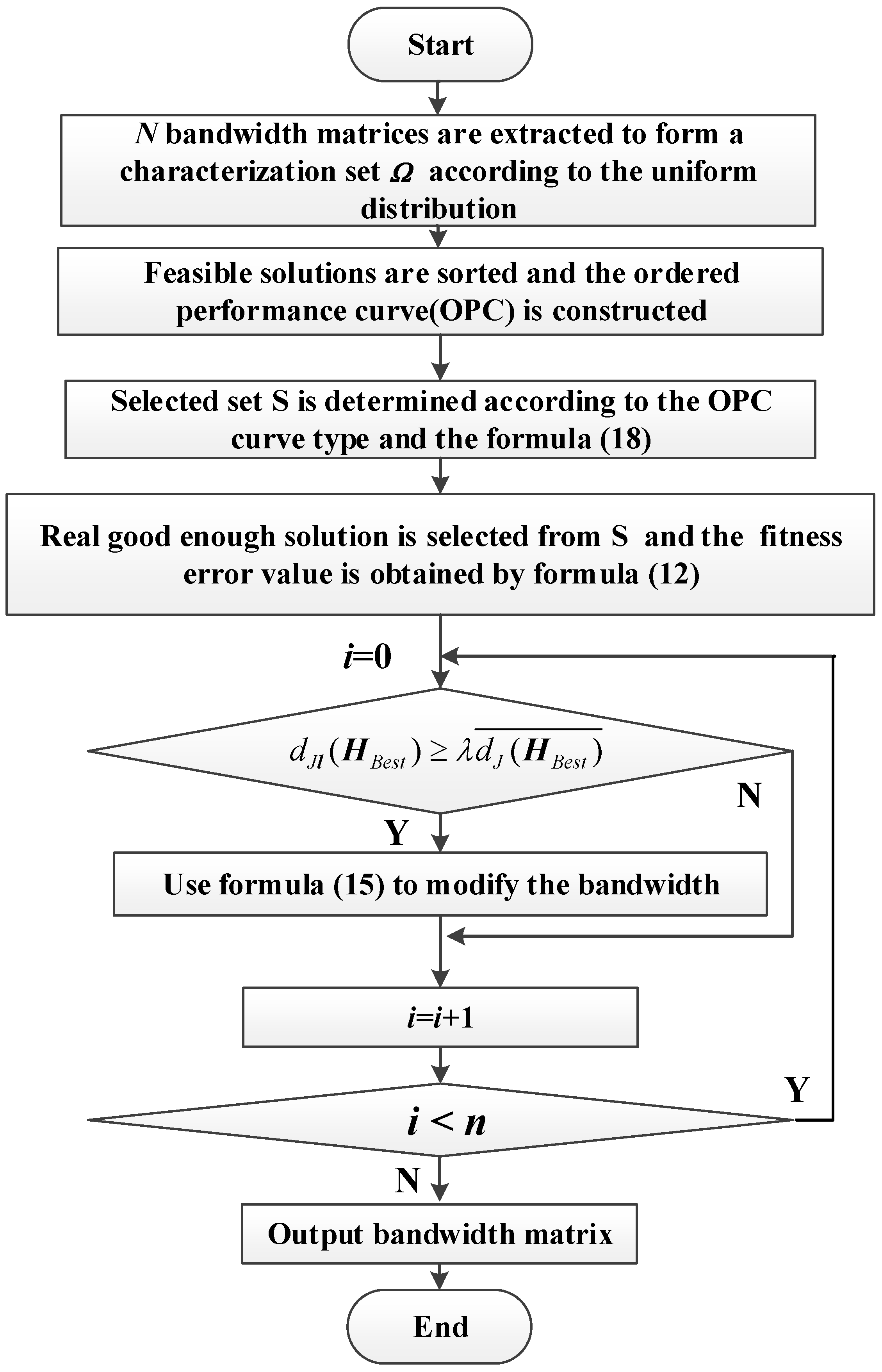
3. Solution of the Optimal Model of Bandwidth Based on Ordinal Optimization

For the proposed AMNKDE in this paper, the bandwidth was transformed from a traditional single parameter matrix, which contributed to the increasing difficulty of the solution. In order to solve this problem, a solving approach of the optimal model of bandwidth, based on OO, was proposed.

OO is an effective method for solving complex optimization problems. According to the previous research in Reference [30], this method was successfully applied to solve the optimal model of bandwidth of univariate NKDE and achieved positive results. In this research, the OO was used to solve the bandwidth optimization problem of AMNKDE, the solution is shown in Figure 1 and the detailed steps are as follows:

(1) In the solution space of the bandwidth matrix H, the N bandwidth matrices were extracted to form a characterization set $\Omega$ according to the uniform distribution. The N was closely related to the size of the solution space. When the solution space was less than 10⁸, N = 1000 was recommended by Reference [46].

(2) The N feasible solutions were selected by the rough model of Formula (10). Then, the feasible solutions were sorted according to the assessment results. In addition, the ordered performance curve (OPC) was constructed. The types of OPC are given in Reference [30].

(3) Formula (18) was used to determine the number of solutions in the selected set S,

$$S=e^{\epsilon }{t}^{\mu }{g}^{\varpi }+\eta ,$$

(18)

where S is the number of solutions in the selected set S, t represents that there exist at least t good enough solutions in the selected set S, g represents the size of the good enough solution subset, $\epsilon ,\mu ,\varpi ,\eta$ are the parameters associated with the type of OPC, and the values are 8.1378, 0.8974, 1.2058, 6.00, respectively [29].

(4) Taking the objective function of Formula (12) as the exact model, the order of comparison of solutions in the solution set S is made and the top t solutions will be selected as real, good enough, solutions.

(5) Utilizing Formula (13), the local sample intervals with low accuracy in the model were found. The bandwidths in these intervals were adjusted according to Formula (15).

4. Scenario Study

In this paper, 4773 sampling sequences of wind power outputs from six wind farms in the Hubei province of China were selected as examples. The sampling time interval was 10 min. The sampling period was from 19:40 on 17 March, 2009 to 23:00 on 19 April, 2009. For the frequency histogram of two wind farms, the straight interval chosen for this paper was 30 kW. For the frequency histogram of three wind farms, the straight interval was 100 kW. For the two wind farms, the total probability density of the samples was $1.1\times {10}^{-3}$. For the three wind farms, the total probability density of the samples was $1\times {10}^{-6}$. When $\lambda =6$, the comprehensive performance of the proposed model was best. The model could improve the overall modeling accuracy by approximately 10% compared with the traditional MNKDE model and the corresponding calculation time was only 63 s. Accordingly, $\lambda =6$ was chosen for this research. According to Reference [47], $\delta$ was 0.79655.

Program simulation was achieved in the MATLAB platform and related computing was completed on a computer with an Intel Core i5-4460 (3.20-GHz) CPU with 8 G of RAM. The computer time of the OO in this paper was 63.350 s. To verify the validity and applicability of the proposed approach, three-dimensional and four-dimensional JPDFs were obtained from two wind farms and three wind farms for comparison and analysis. The active power output sampling sequence of six wind farms is listed in Figure 2.

Figure 2 shows the differences between the output trends of the former three wind farms and those of the latter three wind farms. The differences are most obvious for the sampling points between 1300 and 2300. We concluded that the JPDFs of the former three wind farms and the latter three wind farms are different.

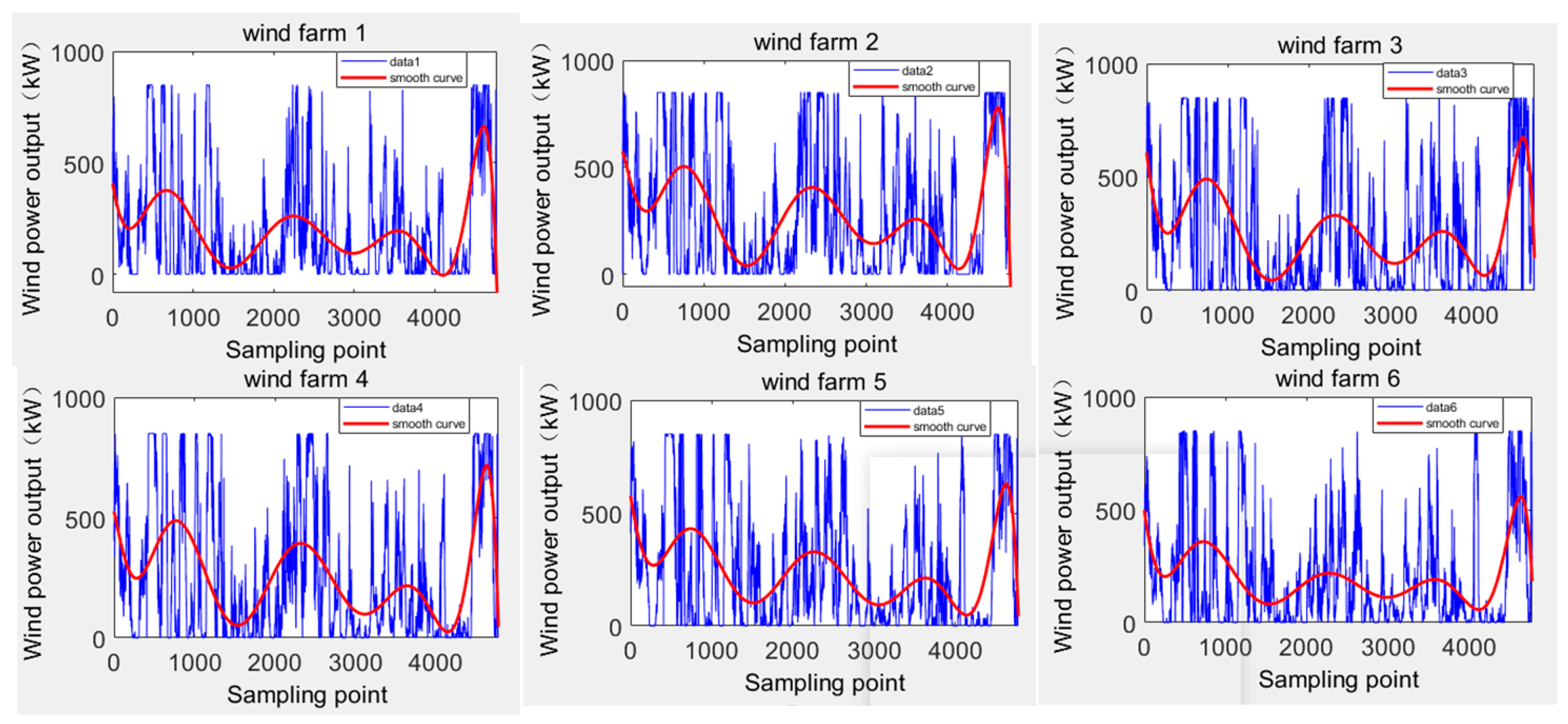
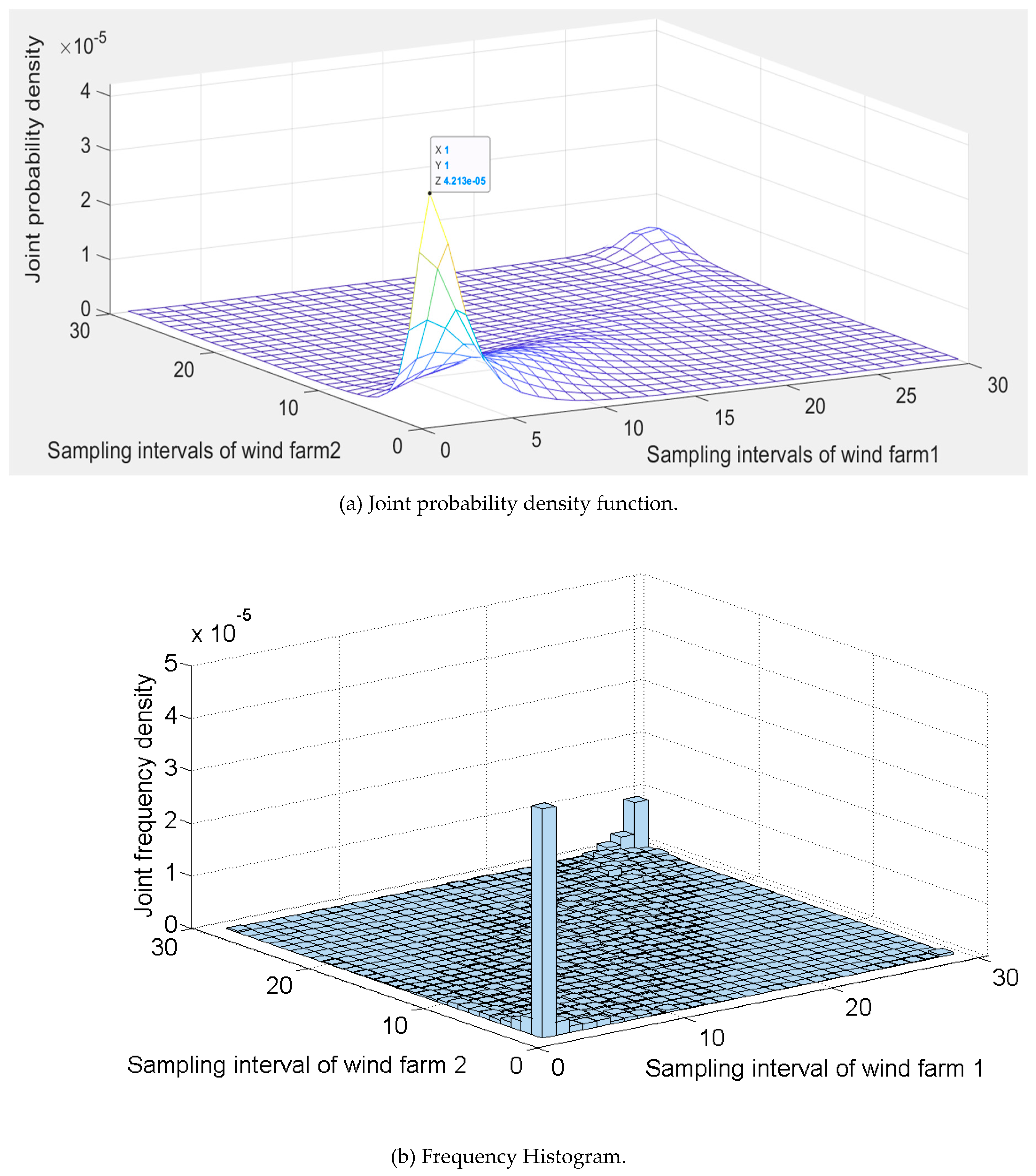
4.1. Joint Probability Density Function Modeling of Two Wind Farms

The JPDF of Wind Farms 1 and 2 were obtained via the approach described previously. The frequency histogram is of Wind Farm 1 and Wind Farm 2, based on the sample data. It is shown in Figure 3b. The comparison between them is shown in Figure 3.

From Figure 3, we found that the outputs of Wind Farms 1 and 2 had a tail correlation. The correlation in the upper tails was stronger, which meant that both wind farms were more likely to produce larger outputs. From the function curve of the model, the modeled JPDF fit well with the real joint distribution of Wind Farms 1 and 2. The detailed calculation results are listed in

Table 1. Detailed calculation results of JPDF for Wind Farms 1 and 2 by AMNKDE.

Model	H	Sample Interval		${\mathit{d}}_{\mathit{O}}$	${\mathit{d}}_{\mathit{M}}$	$\mathit{R}(\mathit{H})$
		Wind Farm 1	Wind Farm 2
AMNKDE	[38.7,38.7]	[30,60]	[30,60]	6.09 × 10−5	4.1 × 10−6	6.50 × 10−5
		[90,900]	[90,900]
	[34.5,34.5]	[0,30]	[0,30]
	[34.7,34.7]	Other interval

.

From the results of Table 1, the modeling error was relatively low and the overall fitness error was only $6.50\times {10}^{-5}$.

4.2. Multipart Figures

To guarantee the generalizability of the results, the four-dimensional JPDF of three wind farms is presented. Based on this scenario, a comparative study was carried out. Models 1, 2, and 3 are the traditional MNKDE model, the AMNKDE model and the comprehensive Copula model, respectively.

4.2.1. Validity Analysis of the Improved Adaptive Strategy for MNKDE

To verify the differences between the proposed AMNKDE and the traditional MNKDE, the JPDFs of Wind Farms 1, 2, and 3 were constructed in these methods. The results are given in

Table 2. Comparison of AMNKDE and MNKDE.

Model	H	Sample Interval			${\mathit{d}}_{\mathit{O}}$	${\mathit{d}}_{\mathit{M}}$	$\mathit{R}(\mathit{H})$
		Wind Farm 1	Wind Farm 2	Wind Farm 3
1	[40.7, 40.7, 40.7]	[0,100]	[0,100]	[0,100]	3.60 $\times$ 10−8	3.60 $\times$ 10−9	7.15 $\times$ 10−8
	[40.7, 40.7, 40.7]	[800,1000]	[800,1000]	[0,100]	3.60 $\times$ 10−8
	[40.7, 40.7, 40.7]	Other interval			2.83 $\times$ 10−8
2	[37,37,37]	[0,100]	[1,100]	[0,100]	3.00 $\times$ 10−8	1.60 $\times$ 10−10	6.52 $\times$ 10−8
	[38,38,38]	[800,1000]	[800,1000]	[0,100]	1.60 $\times$ 10−8
	[40.7,40.7,40.7]	Other interval			3.20 $\times$ 10−8

.

Compared with Model 1, the Euclidean distance, the maximum distance and the overall fitness error of Model 2 were reduced by 6.76%, 55.5% and 8.81%, respectively, as shown in Table 2. This suggests that the modeling accuracy of MNKDE was effectively improved by the new adaptive strategy. The proposed AMNKDE achieved an adaptive improvement for the bandwidths of the sample interval in [0,100] [0,100] [0,100] and [800,1000] [800,1000] [0,100]. The elements of the bandwidth matrices in the sample intervals [0,100] [0,100] [0,100] and [800,1000] [800,1000] [0,100] were changed from 47 to 32 and 33, respectively.

The rest of the interval elements remained as 40.7 and the above matrix as an adaptive bandwidth matrix. The resulting decline of the Euclidean distance for the corresponding sample intervals was 16.7% and 55.6%, respectively. This improvement resulted in a rise of 13.1% in the Euclidean distance of the other sample intervals, but, for the entire sample interval, the overall Euclidean distance and the maximum distance was evidently reduced and the overall fitness error was cut down by 8.81%. We summarized that the overall modeling accuracy of the MNKDE was effectively facilitated by the adaptive bandwidth improvement strategy of the sample intervals with the local adaptability problem.

4.2.2. Accuracy Comparison between AMNKDE and Copula Parameter Estimation

To verify the accuracy of the proposed AMNKDE approach, the JPDF of Wind Farms 1, 2 and 3 were established using the comprehensive Copula method from Reference [29]. The compared results are shown in

Table 3. Accuracy comparison between AMNKDE and Copula parameter estimation.

Model	H	Sample Interval			${\mathit{d}}_{\mathit{O}}$	${\mathit{d}}_{\mathit{M}}$	$\mathit{R}(\mathit{H})$
		Wind Farm 1	Wind Farm 2	Wind Farm 3
1	[40.7, 40.7, 40.7]	[0,100]	[0,100]	[0,100]	3.60 $\times$ 10−8	3.60 $\times$ 10−9	7.15 $\times$ 10−8
	[40.7, 40.7, 40.7]	[800,1000]	[800,1000]	[0,100]	3.60 $\times$ 10−8
	[40.7, 40.7, 40.7]	Other interval			2.83 $\times$ 10−8
2	[37,37,37]	[0,100]	[0,100]	[0,100]	3.00 $\times$ 10−8	1.60 $\times$ 10−10	6.52 $\times$ 10−8
	[38,38,38]	[800,1000]	[800,1000]	[0,100]	1.60 $\times$ 10−8
	[40.7,40.7,40.7]	Other interval			3.20 $\times$ 10−8

. The optimal Copula function was composed of Gumbel Copula, Clayton Copula and Frank Copula.

From Table 3, Model 3, based on the comprehensive Copula method, the Euclidean distance, maximum distance, and overall fitness error of Model 2, based on the proposed AMNKDE approach, were compared and shown to be reduced by 7.8%, 57.9% and 11.6%, respectively. It can be seen that the proposed AMNKDE approach has higher modeling accuracy than the comprehensive Copula method. The reason is that the proposed AMNKDE approach directly models the JPDF based on the sample data. Accordingly, it does not need to choose the specific form of the JPDF in advance and the modeling accuracy is only related to the selection of bandwidth, rather than the prior definition of the JPDF forms.

4.2.3. Comparison of Applicability between AMNKDE and Copula Parameter Estimation

To verify the applicability of the proposed AMNKDE approach, the wind farms were changed for the comparison. The JPDFs of Wind Farms 4, 5, and 6 were established using the AMNKDE and the comprehensive Copula method from Reference [29]. The optimal Copula function still consisted of Gumbel Copula, Clayton Copula and Frank Copula. The detailed results are presented in

Table 4. Comparison of Applicability between AMNKDE and Copula Parameter Estimation.

Model	H	Sample Interval			${\mathit{d}}_{\mathit{O}}$	${\mathit{d}}_{\mathit{M}}$	$\mathit{R}(\mathit{H})$
		Wind Farm 4	Wind Farm 5	Wind Farm 6
2	[38,38,38]	[0,100]	[0,100]	[0,100]	6.78 $\times$ 10−8	1.1 $\times$ 10−10	6.89 $\times$ 10−8
	[39,39,39]	[800,1000]	[800,900]	[0,100]
	[41.7,41.7,41.7]	Other interval
3	Copula function	$\lambda$		$\theta$	7.83 $\times$ 10−8	2.50 $\times$ 10−9	8.08 $\times$ 10−8
	Gumbel	0.386		5.60
	Clayton	0.403		4.940
	Frank	0.211		8.586

.

From Table 4, the proposed AMNKDE approach still maintained high modeling accuracy for the different wind farms. Compared with Table 3, the overall fitness error of the AMNKDE increased by 5.67%. In contrast, the overall fitness error increase of the comprehensive Copula method was larger, 10.99%, and the increase was 1.94 times that of the AMNKDE. It can be concluded that the proposed AMNKDE approach possesses high applicability compared with the Copula PE method when the modeling object is changed. The reason is that the latter method needs to judge the form of the JPDF, and the joint probability distribution of different wind farms may follow different function forms. Consequently, it may cause a large error if the same function form is used to model different wind farms.

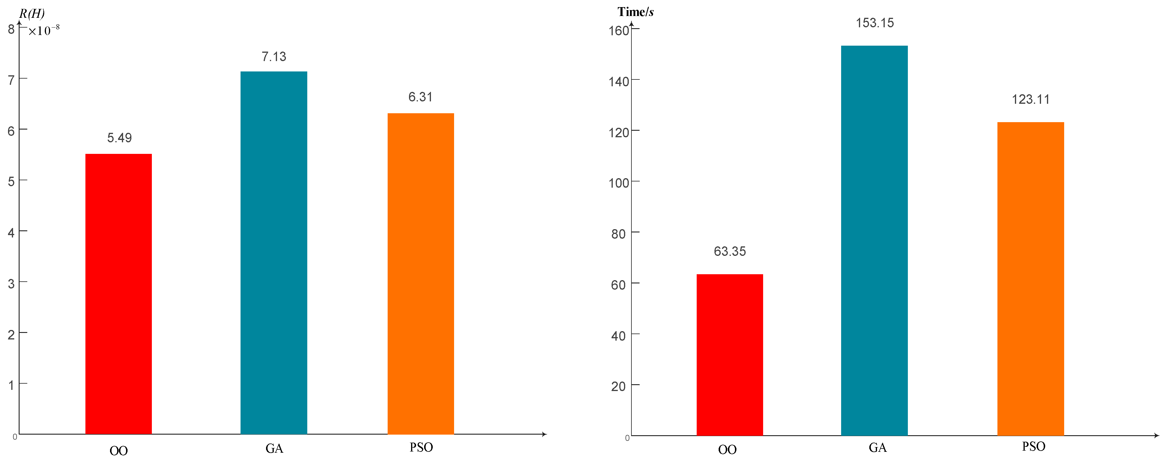
4.2.4. Comparison of Algorithms

To analyze the validity of the OO algorithm in this paper, the calculation efficiency was proposed. The GA, PSO and OO algorithms were used to solve the optimal model of bandwidth in this paper. The optimal bandwidth matrices of these three algorithms, ${\mathit{H}}_{best}$, were [48.7,48.7,48.7], [55,55,55], [52,52,52], respectively. The results of the fitness error $R(\mathit{H})$ and the computation time are shown in Figure 4.

Figure 4 compares the traditional genetic algorithm and the PSO algorithm. The proposed OO algorithm was relatively limited in terms of improving the computational accuracy. However, the OO possessed a significant advantage in computational efficiency. It can be concluded that the proposed OO algorithm can effectively guarantee the computational efficiency and accuracy.

5. Conclusions

As the accuracy and applicability of many JPDF modeling methods for multiple wind farms need to be improved, it is of significance to promote the accuracy and applicability of the modeling method of JPDF. This is exactly the purpose of this study.

The specific steps of AMNKDE are as follows. First, the model of AMNKDE was constructed using the optimal bandwidth. Second, an optimal model of bandwidth based on Euclidean distance and maximum distance was constructed and the comprehensive minimum of these distances was used as a measure of optimal bandwidth. Finally, the OO algorithm was used to solve this model.

The specific conclusions of this paper are as follows:

(1) The adaptive bandwidth improvement strategy proposed in this paper replaces the traditional fixed bandwidth of MNKDE with the adaptive bandwidth. It effectively facilitates the overall modeling accuracy of MNKDE by adjusting the bandwidth of local sample interval adaptively. Simulation results in this paper indicate that the overall fitness error of AMNKDE was 8.81% lower than that of traditional MNKDE.

(2) Based on the above strategy, an AMNKDE approach was proposed and utilized to build the JPDF model for multiple wind farms. The simulation results in this paper indicated that the overall fitness error of AMNKDE was 11.6% lower than that of Copula-based PE method. After replacing the modeling object the overall fitness error of the comprehensive Copula method increased by as much as 1.94 times that of AMNKDE. Consequently, the accuracy and applicability of the AMNKDE approach were better than that of the traditional Copula PE method.

In summary, the proposed AMNKDE approach clearly performed better than MNKDE and Copula hybrid models and was suitable for building a multi-wind farm joint probability density model.

This study can be further extended. The proposed approach in this paper can be further applied to many other fields of uncertain modeling, such as the JPDF modeling problems of photovoltaic power systems and wind-solar combined power systems.

References

1. Wu, J.; Zhang, B.; Wang, K. Optimal economic dispatch model based on risk management for wind-integrated power system. IET Gener. Transm. Distrib. 2015, 9, 2152–2158. [Google Scholar] [CrossRef]
2. Hu, D.; Ryan, S.M. Stochastic vs. deterministic scheduling of a combined natural gas and power system with uncertain wind energy. Int. J. Electr. Power Energy Syst. 2019, 108, 303–313. [Google Scholar] [CrossRef]
3. Yan, J.; Liu, Y.; Han, S. Reviews on uncertainty analysis of wind power forecasting. Renew. Sustain. Energy Rev. 2015, 52, 1322–1330. [Google Scholar] [CrossRef]
4. Zhang, Y.; Jian, L.; Zheng, F.; Zhang, Y.; Liu, K. Two-stage distributionally robust coordinated scheduling for gas-electricity integrated energy system considering wind power uncertainty and reserve capacity configuration. Renew. Energy 2019, 135, 122–135. [Google Scholar] [CrossRef]
5. Wu, J.; Zhang, B.; Jiang, Y.; Bie, P.; Li, H. Chance-constrained stochastic congestion management of power systems considering uncertainty of wind power and demand side response. Int. J. Electr. Power Energy Syst. 2019, 107, 703–714. [Google Scholar] [CrossRef]
6. Dvorkin, Y.; Lubin, M.; Backhaus, S. Uncertainty Sets for wind power generation. IEEE Trans. Power Syst. 2016, 31, 3326–3327. [Google Scholar] [CrossRef]
7. Wang, B.; Fang, B.; Wang, Y.; Liu, H.; Liu, Y. Power System Transient Stability Assessment Based on Big Data and the Core Vector Machine. IEEE Trans. Smart Grid 2016, 7, 2561–2570. [Google Scholar] [CrossRef]
8. Liu, R.; Peng, M.; Xiao, X. Ultra-Short-Term Wind Power Prediction Based on Multivariate Phase Space Reconstruction and Multivariate Linear Regression. Energies 2018, 11, 2763. [Google Scholar] [CrossRef]
9. Li, J.; Wang, S.; Ye, L.; Fang, J. A coordinated dispatch method with pumped-storage and battery-storage for compensating the variation of wind power. Prot. Control Mod. Power Syst. 2018, 3, 21–34. [Google Scholar] [CrossRef]
10. Zheng, D.; Eseye, A.; Zhang, J.; Li, H. Short-term wind power forecasting using a double-stage hierarchical ANFIS approach for energy management in microgrids. Prot. Control Mod. Power Syst. 2017, 2, 136–145. [Google Scholar] [CrossRef]
11. Liao, S.; Xu, J.; Sun, Y. Control of Energy-intensive Load for Power Smoothing in Wind Power Plants. IEEE Trans. Power Syst. 2018, 33, 6142–6154. [Google Scholar] [CrossRef]
12. Yang, H.; Xie, K.; Tai, H.M. Wind farm layout optimization and its application to power system reliability analysis. IEEE Trans. Power Syst. 2016, 31, 2135–2143. [Google Scholar] [CrossRef]
13. Tian, P.C. Estimation of wind energy potential using different probability density functions. Appl. Energy 2011, 88, 1848–1856. [Google Scholar]
14. Altunkaynak, A.; Erdik, T.; Dabanlı, İ.; Şen, Z. Theoretical derivation of wind power probability distribution function and applications. Appl. Energy 2012, 92, 809–814. [Google Scholar] [CrossRef]
15. Tina, G.; Gagliano, S. Probabilistic analysis of weather data for a hybrid solar/wind energy system. Int. J. Energy Res. 2011, 35, 221–232. [Google Scholar] [CrossRef]
16. Wang, C.; Li, X.H.; Tian, T.; Xu, Z.R.; Chen, R. Coordinated control of passive transition from grid-connected to islanded operation for three/single-phase hybrid multimicrogrids considering speed and smoothness. IEEE Trans. Ind. Electron. 2019. [Google Scholar] [CrossRef]
17. Liu, T.H.; Wei, H.K.; Zhang, K.J. Wind power prediction with missing data using Gaussian process regression and multiple imputation. Appl. Soft Comput. 2018, 71, 905–916. [Google Scholar] [CrossRef]
18. Yin, H.; Zivanovic, R. Using probabilistic collocation method for neighbouring wind farms modeling and power flow computation of South Australia grid. IET Gener. Transm. Distrib. 2017, 11, 3568–3575. [Google Scholar] [CrossRef]
19. Zhang, L.; Luo, Y. Combined Heat and Power Scheduling: Utilizing Building-level Thermal Inertia for Short-term Thermal Energy Storage in District Heat System. IEEE Trans. Electr. Electron. Eng. 2018, 13, 804–814. [Google Scholar] [CrossRef]
20. Olauson, J.; Bergkvist, M. Correlation between wind power generation in the European countries. Energy 2016, 114, 663–670. [Google Scholar] [CrossRef]
21. Luo, G.; Chen, J.; Cai, D. Probabilistic assessment of available transfer capability considering spatial correlation in wind power integrated system. IET Gener. Transm. Distrib. 2013, 7, 1527–1535. [Google Scholar]
22. Xie, Z.Q.; Ji, T.Y.; Li, M.S. Quasi-Monte carlo based probabilistic optimal power flow considering the correlation of wind speeds using Copula function. IEEE Trans. Power Syst. 2018, 33, 2239–2247. [Google Scholar] [CrossRef]
23. Li, C.X.; Dong, Z.Y.; Chen, G. Flexible transmission expansion planning associated with large-scale wind farms integration considering demand response. IET Gener. Transm. Distrib. 2015, 9, 2276–2283. [Google Scholar] [CrossRef]
24. Hu, B.Q.; Wu, L.; Marwali, M. On the robust solution to scuc with load and wind uncertainty correlations. IEEE Trans. Power Syst. 2014, 29, 2952–2964. [Google Scholar] [CrossRef]
25. Papaefthymiou, G.; Kurowicka, D. Using Copulas for modeling stochastic dependence in power system uncertainty analysis. IEEE Trans. Power Syst. 2009, 24, 40–49. [Google Scholar] [CrossRef]
26. Gill, S.; Stephen, B.; Galloway, S. Wind Turbine Condition Assessment Through Power Curve Copula Modeling. IEEE Trans. Sustain. Energy 2012, 3, 94–101. [Google Scholar] [CrossRef] [Green Version]
27. Louie, H. Evaluation of bivariate archimedean and elliptical Copulas to model wind power dependency structures. Wind Energy 2014, 17, 225–240. [Google Scholar] [CrossRef]
28. Zhang, J.; Chowdhury, S.; Messac, A. A Multivariate and Multimodal Wind Distribution model. Renew. Energy Int. J. 2013, 51, 436–447. [Google Scholar] [CrossRef]
29. Wang, J.W.; Zhou, B.X.; Li, H.B. Modeling of wind farm output correlation based on comprehensive Copula function. Electr. Meas. Instrum. 2016, 53, 100–105. [Google Scholar]
30. Yang, N.; Cui, J.Z.; Zhou, Z. Research on nonparametric kernel density estimation for modeling of wind power probability characteristics based on fuzzy ordinal optimization. Power Syst. Technol. 2014, 40, 335–340. [Google Scholar]
31. Yang, N.; Ye, D.; Zhou, Z.; Cui, J.Z.; Chen, D.J.; Wang, X.M. Research on modelling and solution of stochastic SCUC under AC power flow constraints. IET Gener. Transm. Distrib. 2018, 12, 3618–3625. [Google Scholar]
32. Soleimanpour, N.; Mohammadi, M. Probabilistic load flow by using nonparametric density estimators. IEEE Trans. Power Syst. 2013, 28, 3747–3755. [Google Scholar] [CrossRef]
33. Ren, Z.Y.; Yan, W.; Zhao, X. Chronological probability model of photovoltaic generation. IEEE Trans. Power Syst. 2014, 29, 1077–1088. [Google Scholar] [CrossRef]
34. Carbone, P.; Petri, D.; Barbé, K. Nonparametric probability density estimation via interpolation filtering. IEEE Trans. Instrum. Meas. 2017, 66, 681–690. [Google Scholar] [CrossRef]
35. Zhu, B.X.; Ren, L.L.; Hu, X. Kind of high step-up dc/dc converter using a novel voltage multiplier cell. IET Power Electron. 2017, 10, 129–133. [Google Scholar] [CrossRef]
36. Kristan, M.; Leonardis, A.; Skoc, D. Multivariate online kernel density estimation with Gaussian kernels. Pattern Recognit. 2011, 44, 2630–2642. [Google Scholar] [CrossRef]
37. Li, Z.H.; Tao, Y.; Abu-Siada, A. A New Vibration Testing Platform for Electronic Current Transformers. IEEE Trans. Instrum. Meas. 2019, 68, 704–712. [Google Scholar] [CrossRef]
38. Pulkkinen, S.; Mäkelä, M.; Karmitsa, N. A continuation approach to mode-finding of multivariate Gaussian mixtures and kernel density estimates. J. Glob. Optim. 2013, 56, 459–487. [Google Scholar] [CrossRef]
39. Chang, M.S.; Wu, X.M. Transformation-based nonparametric estimation of multivariate densities. J. Multivar. Anal. 2015, 135, 71–88. [Google Scholar] [CrossRef]
40. Gramacki, A.; Gramacki, J. FFT-based fast computation of multivariate kernel density estimators with unconstrained bandwidth matrices. J. Comput. Graph. Stat. 2017, 26, 459–462. [Google Scholar] [CrossRef]
41. Zhao, Y.; Zhang, X.F.; Zhou, J.Q. Load Modeling Utilizing Nonparametric and Multivariate Kernel Density Estimation in Bulk Power System Reliability Evaluation. Proc. CSEE 2009, 29, 27–33. [Google Scholar]
42. Zougab, N.; Smail, K.; Célestin, C. Bayesian estimation of adaptive bandwidth matrices in multivariate kernel density estimation. Comput. Stat. Data Anal. 2014, 75, 28–38. [Google Scholar] [CrossRef]
43. Sreevani, N.; Murthy, C.A. On bandwidth selection using minimal spanning tree for kernel density estimation. Comput. Stat. Data Anal. 2016, 102, 67–84. [Google Scholar] [CrossRef]
44. Zhao, Y.; Yang, J.G.; Li, S.X. Nonparametric disaggregation load model in power system reliability evaluation incorporating the additive correlation. IEEE Trans. Power Syst. 2008, 23, 6039–6047. [Google Scholar]
45. Van Kerm, P.; Mohammadi, M. Adaptive kernel density estimation. Stata J. 2003, 3, 148–156. [Google Scholar] [CrossRef]
46. Liu, Y.S.; Lin, J.K.; Guo, L.X. A robust state estimation method based on adaptive kernel density estimation Theory. Proc. CSEE 2012, 19, 4937–4946. [Google Scholar]
47. Epanecnikov, V.A. Nonparametric estimation of a multidimensional probability density. Theory Probab. Appl. 2003, 14, 156–161. [Google Scholar]
Figure 1. Flow Chat for the Solution.
Energies 12 01356 g001
Figure 2. Historical data of six wind farms.
Energies 12 01356 g002
Figure 3. Joint probability density function and frequency histogram of Wind Farms 1 and 2.
Energies 12 01356 g003
Figure 4. Comparison of Accuracy and Operation Time between Different Algorithms.
Energies 12 01356 g004