Optimal Coordination of Aggregated Hydro-Storage with Residential Demand Response in Highly Renewable Generation Power System: The Case Study of Finland

Abstract

Current energy policy-driven targets have led to increasing deployment of renewable energy sources in electrical grids. However, due to the limited flexibility of current power systems, the rapidly growing number of installations of renewable energy systems has resulted in rising levels of generation curtailments. This paper probes the benefits of simultaneously coordinating aggregated hydro-reservoir storage with residential demand response (DR) for mitigating both load and generation curtailments in highly renewable generation power systems. DR services are provided by electric water heaters, thermal storages, electric vehicles, and heating, ventilation and air-conditioning (HVAC) loads. Accordingly, an optimization model is presented to minimize the mismatch between demand and supply in the Finnish power system. The model considers proportions of base-load generation comprising nuclear, and combined heat and power (CHP) plants (both CHP-city and CHP-industry), as well as future penetration scenarios of solar and wind power that are constructed, reflecting the present generation structure in Finland. The findings show that DR coordinated with hydropower is an efficient curtailment mitigation tool given the uncertainty in renewable generation. A comprehensive sensitivity analysis is also carried out to depict how higher penetration can reduce carbon emissions from electricity co-generation in the near future.

1. Introduction

Recently, the European Union (EU) issued energy efficiency directives to effectively address and eradicate the worst effects of climate change. In this respect, the EU-2030 climate and energy framework has set key targets that include a 40% reduction in greenhouse gas (GHG) emissions relative to 1990 levels, a 27% reduction in total energy consumption, and a minimum 27% share of renewable energy sources (RESs) in the entire EU by 2030 [1]. Similarly, more ambitious goals concerning GHG emission reductions have been set for the EU-2050 energy roadmap.

Hence, such environmental and energy policies have substantially increased the share of RESs, particularly wind and solar generation, in the total generation mix worldwide. The central objective of these policies is to achieve a carbon neutral system by replacing fossil fuel based conventional generation with renewables, as these are emission free. However, integration of RESs poses a challenge to the current grid owing to the un-dispatch-able nature of many RESs. Due to the intermittency of RESs and their lack of flexibility, maintaining power system balance becomes challenging and often results in curtailment events. For instance, 1166 GWh of wind generation was curtailed in Spain in 2013 [2]. Such events imply that the power system could not realize the potential benefits of the investment in RESs and failed to reduce GHG emissions. Moreover, the cost of such curtailments is borne by the system in the form of increased tariffs.

Solutions to integrate RESs include storage technologies, market price strategies, support schemes, and demand response (DR). The merits and de-merits of these options have been widely discussed in the literature. Storage technologies, such as pumped hydro storage or compressed air storage, need huge investment cost [3]. Moreover, for the time being, the price volatility in Nord-Pool is not favorable for storages to cover the marginal cost of charge and discharge through price arbitrage [3]. Similarly, markets introduce negative pricing during events of high generation, thus paying consumers to consume the excess output of RESs. Depending on the magnitude of surplus production, the high negative price may not be enough to balance the market by price only [2]. Support schemes e.g., priority dispatch for RESs, work counter to open market conditions, conflict heavily with EU market liberalization policy. Due to such limitations, DR is considered the most economical and potential tool compared to other options. It has a tendency to act as a power resource or power sink depending on the generation profile.

In this context, several studies have focused on the flexibility offered by various DR loads. For instance, Reference [4] studied the distributed control of DR offered by heating, ventilation and air-conditioning (HVAC), and electric water heater (EWH) loads in smart grids. The work in Reference [5] demonstrated the benefits of HVAC DR coordinated with thermal storage for wind generation balancing. Similarly, the temporal matching of local loads with on-site photovoltaic generation was maximized with the aid of flexible loads in [6]. A framework to jointly optimize the scheduling of HVAC loads and electric vehicles (EVs) was proposed in [7]. The benefits offered by DR in distribution systems was reported in [8]. In Reference [9], the potential benefits of HVAC DR coordinated with thermal masses were studied in a Micro-grid participating in a two-stage electricity market.

Moreover, numerous studies have been performed to integrate high wind power into the system while utilizing the flexibility offered by responsive loads. In Reference [10], the flexibility of HVAC loads coordinated with building thermal masses were studied to mitigate the curtailments in islanded networks. The power sink capabilities of HVAC and EV loads under variable wind generation penetrations were analyzed in [11]. In Reference [12], a framework was proposed to jointly minimize energy cost and wind generation curtailment using aggregated DR services in a distribution system. The authors in Reference [13] quantified the system-wide storage size required for renewable generation curtailment mitigation in the Finnish power system. The system’s storage was aided by residential DR through electric storage space heaters. Although the study targeted future grids, it neglected to consider hydro-generation and load curtailment issue. Similarly, DR potential of electric storage space heaters was analyzed in [14] to address wind generation curtailment under different penetrations, but the crucial details of base-load generation were not considered. The work in Reference [15] devised a methodology to utilize the flexibility of combined heat and power (CHP) production to integrate wind power in the grid. A major drawback was that the wind integration was accomplished at the expense of increased carbon emissions. Researchers in [16] followed a model-based approach to quantify the upper limit of wind curtailments for the future power system of Ireland. The approach in [16] neither considered details of system demand nor generation mix.

In order to integrate RESs into power systems, both load and generation curtailments need to be addressed in the problem. Existing studies in this field do not realize all the aspects and details of the load and generation mix which are required to analyze the emission reduction in a power system. The scope of this work is to investigate the power system balance under high penetrations of solar and wind generation over and above the mix of base-load generation in Finland. The base-load generation comprises nuclear and CHP co-generation. The objective is to simultaneously minimize load and RES curtailments system-wide, and investigate the options of mitigating such RES curtailments in case high RES penetration is required for emission-free power system in Finland. To achieve this, the flexibility of aggregated hydro-storage was utilized while probing the DR services offered by the residential sector, which constitutes about 25% of the total electricity consumption in Finland. A smart grid communication environment is assumed where the system operator is authorized for direct load control of residential consumers through the home energy management system (HEMS).

For DR, we considered HVAC, EWH, thermal storage, and EV charging loads. The reason for selecting these loads is their chief contribution to annual residential demand. For instance, space heating load alone represents about 70% of the residential demand, and is mainly due to the long winter season in Finland. The central idea underlying HVAC DR is that users can tolerate a small deviation from set point temperatures. The HVAC load can be scheduled to follow an intermittent RES profile by preheating or pre-cooling the buildings. Building thermal masses, due to high thermal time constant, enable effective management of the HVAC response. Moreover, the domestic storage space heater (space heater equipped with a thermal storage) is another DR example. Similarly, EWH is an essential component for domestic hot water (DHW) consumption. The DHW storage for EWH may be integrated into thermal storage of space heaters, which is ubiquitous in Finland, but here both are studied apart. EV charging can be flexibly scheduled as long as the demand is satisfied for the next journey.

The remainder of the paper is structured as follows. Section 2 discusses the generation and load models followed in this study. Section 3 details the mathematical formulation. Section 4 discusses the simulation results while the paper is concluded in Section 5.

2. Modeling Methodology

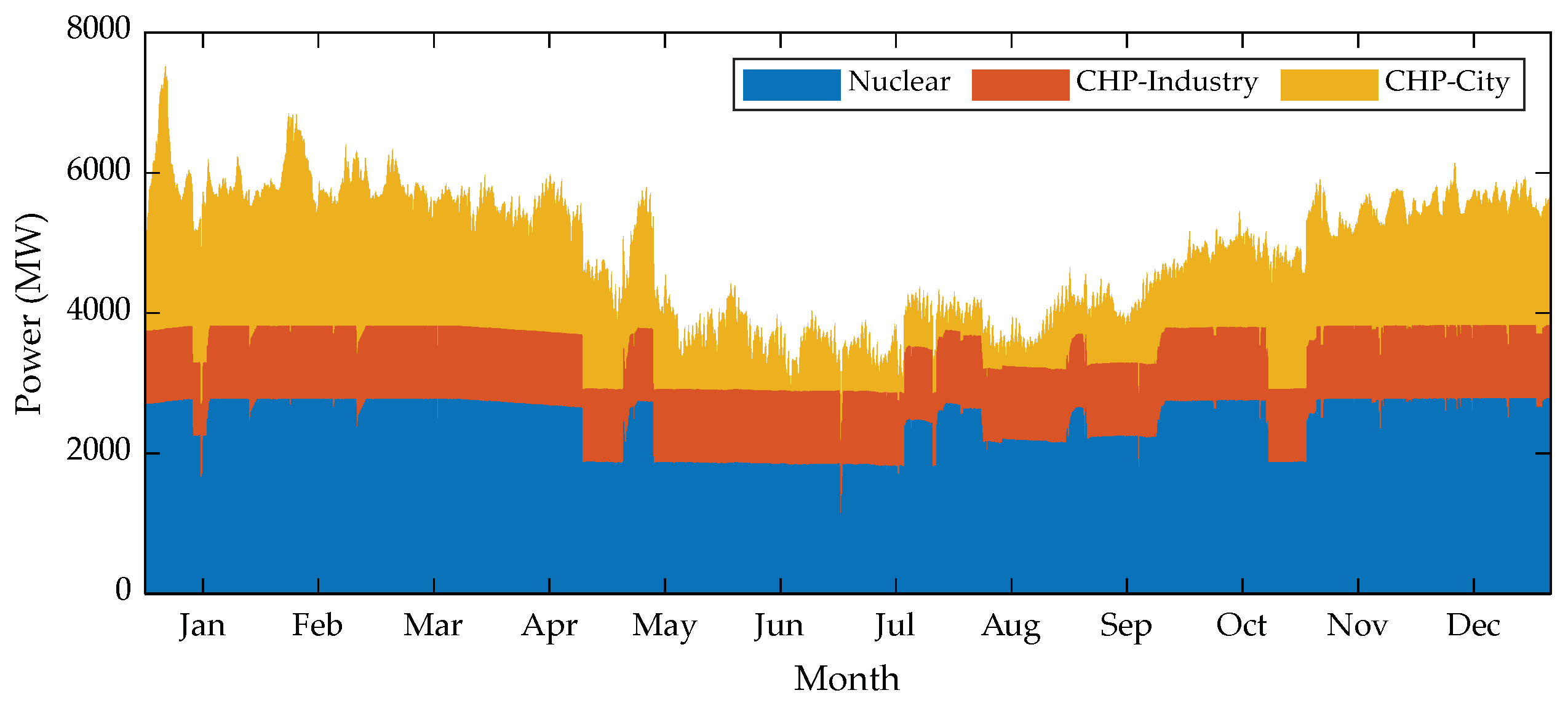
2.1. Base-Load Generation Modeling

In Finland, base-load generation comprises nuclear, as well as CHP plants. CHP plants serve both the city and industry. Nuclear power plants offer almost a constant aggregated generation level with a few maintenance breaks for different units during summer season. CHP-industry also operates on a constant level and is integrated in the pulping process thus being largely based on bio-fuels. CHP-city electricity production follows the trend of seasonal heat demand of Finnish building stock. It serves the building stock via district heating networks whereas the electricity co-generation is sold to the market or grid. In winter, the electricity production is high as heat demand is high and in summer, vice versa. Knowing the aggregated annual electrical production of CHP-city plants, power to heat ratios and the total building stock, the electrical generation profile can be simulated with a good accuracy using data available at [17,18].

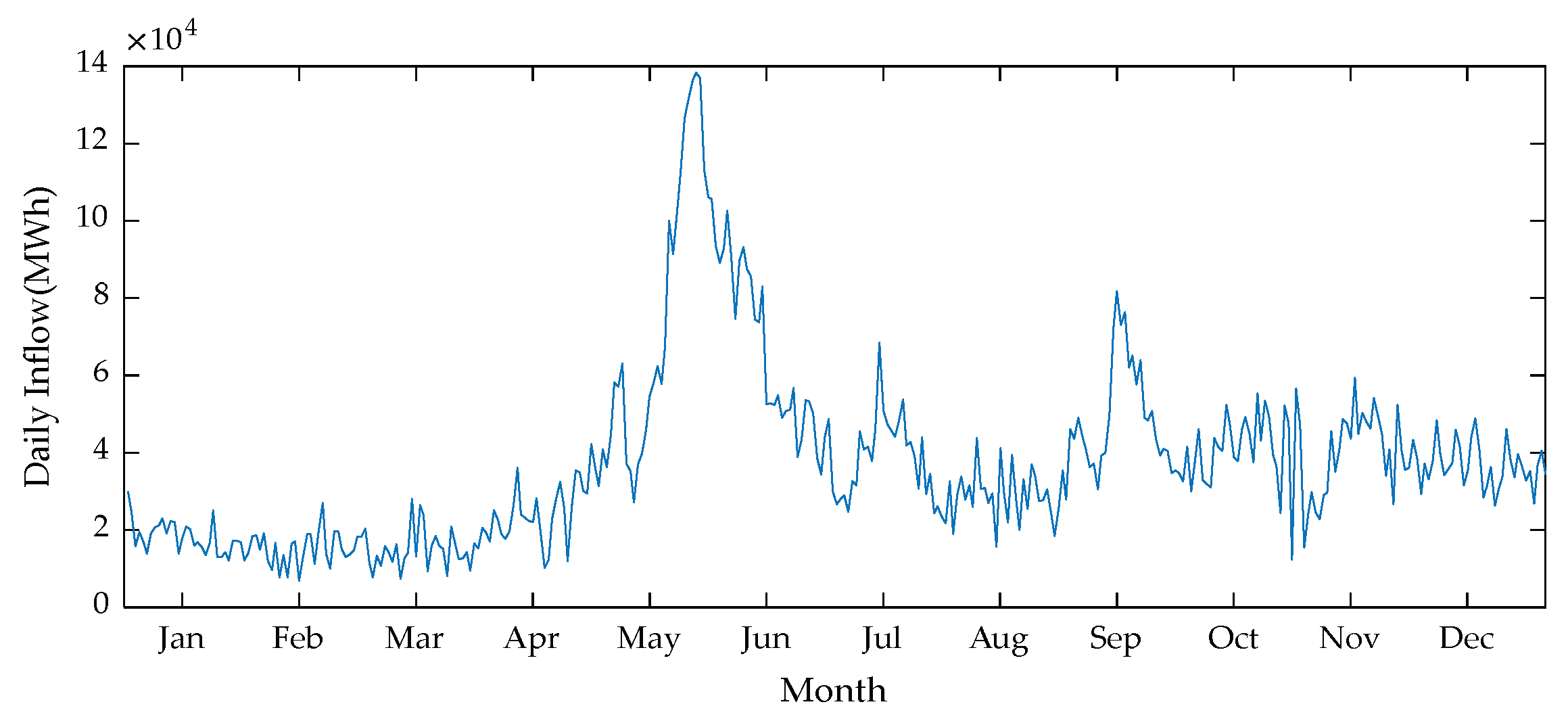
2.2. Hydro-Generation Modeling

We model the hydro-generation using equivalent energy values of aggregated hydro-reservoir capacity, daily water inflows, and minimum and maximum dispatch levels of hydro-generation. In terms of electrical energy, the total hydro storage capacity across Finland is 5530 GWh. The daily energy inflow to the reservoirs in Finland for the year 2017 is available at Nord-pool spot [19] as illustrated in Figure 1. Nord-Pool is a multinational power exchange for electricity trade in the Nordic region. All cross border trade takes place in Nord-Pool. It originated as a power exchange for Norway and eventually Sweden, Finland, Denmark, Estonia, and other Baltic countries also integrated in it.

The source of inflows mainly includes the melting of snow and rainfalls, which is notable in the Figure. The highest peak occurs when the snow melts in May, while the smaller peak is in the rainy season. The minimum dispatch level of hydro generation has to be maintained to allow the use of water for agricultural purposes, while the maximum dispatch level is constrained by the installed hydro-generation capacity in Finland. The minimum and maximum dispatch levels for hydro generation are 422 MW and 2550 MW, respectively.

2.3. Renewable Generation Modeling

This work requires realistic wind and photovoltaic (PV) generation time series for future penetration scenarios in Finland. Wind generation can be modeled using a statistical approach that combines probability integral transformation and simulated wind speed time series for new generation locations without any measurement data as proposed in [20]. On the other hand, PV generation can be modeled with similar methodology aimed to produce power time series for new PV locations without measurement data as presented in [21]. A joint modeling of both wind and PV is utilized here as followed in [13]. The obtained aggregated generation series is well suitable for long-term future studies.

The approach for wind generation considers the actual geography and installed wind power generation structures of Finland in the beginning of 2016. The existing wind farms were expanded proportionally to include new turbines with latest technology available at that time. The upscaling factor was determined according to the aggregated electricity generation in Finland during 2015, including net imports. For PV generation, 12 locations, with equal installed capacity were considered, distributed in southern Finland. The average capacity factor for aggregated wind and PV generation was 28% and 11.8%, respectively.

Using the methodology, 100 runs were simulated for a one-year period. Of these scenarios, a well above average scenario within the 95th percentile was selected for this work. A sensitivity analysis was also carried out due to the uncertainty in intermittent generation.

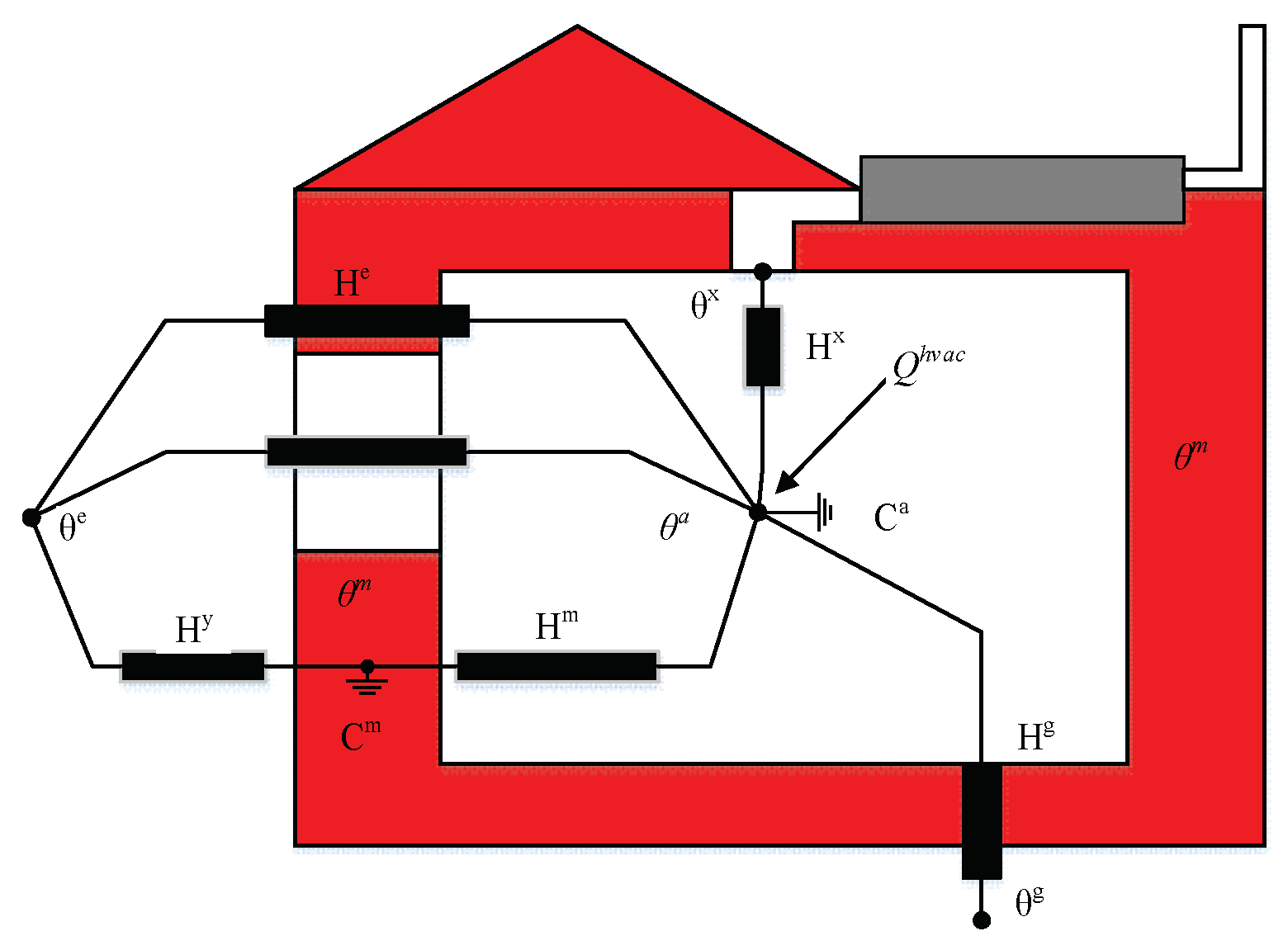
2.4. Two-Capacity Building Model for HVAC Loads

To estimate the heating or cooling requirements in a detached house, we utilized a two-capacity model from our previous works [6,13,22]. This thermal model studies the indoor temperature variation with respect to the external temperature. As the name suggests, it requires two heat capacitances. One capacitance is allocated to the building mass, C^m, whereas the other is distributed to the indoor air, C^a. While C^a is much smaller than C^m, it plays an inevitable role in assessing the indoor air dynamics. This model has two unknown temperature variables, namely, the indoor temperature, θ^a, and the building mass temperature, θ^m. Figure 2 illustrates this model.

It is assumed that the HVAC unit, responsible for the ventilation air flows, is set to operate at a constant temperature, θ^x. The generated air is of convective type and is allocated to the indoor air node. For heat flows, the ground temperature, θ^g, must be considered. The windows installed in the building have a small thermal mass compared to the building envelope. The different node points and the HVAC unit are connected through heat conductance, or whenever there is heat flow, they are connected by heat capacity. The building mass node is located at a vague depth inside the building and hence represents the average temperature of the building mass. It is assumed that the internal heat transfer by electric appliances and occupants is negligible.

Unknown building parameters were identified by comparing the step response of the IDA (IDA is a simulation tool to study the indoor environment and energy consumption of a building) model and two-capacity model. The HVAC power was followed by a six-hour interruption resulting in an exponential decay of θ^a. The parameters were determined by minimizing the difference between the response from IDA and two-capacity model.

2.5. Electric Vehicle

The driving behavior and trip lengths of an EV are rather random and require Monte Carlo simulation. This travel information can be transmitted by EV drivers to the aggregator before the scheduling day, thanks to the smart grid communication. For this study, we employed the Finnish National Travel Survey (NTS) [23] that offers starting time probabilities of journeys related to different age groups and their trip lengths corresponding to different week-days. This data can be combined and used to generate different EV profiles in Finland similar to the approach in [24]. Using travel efficiency and battery capacity of an EV available with the manufacturer, this driving routine can be converted into electricity charging demand accordingly. For the sake of simplicity here, a weekday is considered given that people drive to working and public locations. It is assumed that charging facilities are available only at homes. For the business as usual case, the EV is plugged-in for charging as soon as it reaches its parking destination at home. If DR is enabled, charging can be deferred or shifted as long as the battery has enough storage to cover the demand for the next journey. Only grid to vehicle (G2V) mode is studied in this work.

3. Mathematical Formulation

This section presents the mathematical modeling for the proposed framework. The objective is to minimize both the load and RES curtailments based on the flexibility offered by hydro storage and flexible residential loads, as stated in Equation (1):

$$Minimize{\displaystyle \sum _t\left|\left({{\displaystyle P}}_t^{Nuclear}+{{\displaystyle P}}_t^{CHP-city}+{{\displaystyle P}}_t^{CHP-ind}+{{\displaystyle P}}_t^{hydro}+{{\displaystyle P}}_t^{REN}\right)-\left({{\displaystyle D}}_t^{Critical}+{{\displaystyle D}}_t^{Flex}\right)\right|}\Delta t,\forall t\in T$$

(1)

The first term in Equation (1) represents the total generation and the last term represents the total load to be satisfied. The above objective is subject to some constraints discussed hereafter.

$${{\displaystyle D}}_t^{Flex}={{\displaystyle D}}_t^{HVAC}+{{\displaystyle D}}_t^{EWH}+{{\displaystyle D}}_t^{EV},\forall t\in T$$

(2)

$${{\displaystyle \theta }}_{t,n}^a=\frac{{{\displaystyle \theta }}_{t-1,n}^a+\frac{\Delta t}{{{\displaystyle C}}^a}\left({{\displaystyle {{\displaystyle H}}^m\theta }}_{t-1,n}^m+{{\displaystyle {{\displaystyle H}}^e\theta }}_{t,n}^e+{{\displaystyle {{\displaystyle H}}^g\theta }}_{t,n}^g+{{\displaystyle {{\displaystyle H}}^x\theta }}_{t,n}^x+{{\displaystyle Q}}_{t,n}^{hvac}\right)}{1+\frac{\Delta t}{{{\displaystyle C}}^a}\left({{\displaystyle H}}^m+{{\displaystyle H}}^e+{{\displaystyle H}}^g+{{\displaystyle H}}^x\right)},\forall t\in T,\forall n\in N$$

(3)

$${{\displaystyle \theta }}_{t,n}^m=\frac{{{\displaystyle \theta }}_{t-1,n}^m+\frac{\Delta t}{{{\displaystyle C}}^m}\left({{\displaystyle {{\displaystyle H}}^m\theta }}_{t-1,n}^a+{{\displaystyle {{\displaystyle H}}^y\theta }}_t^e\right)}{1+\frac{\Delta t}{{{\displaystyle C}}^m}\left({{\displaystyle H}}^m+{{\displaystyle H}}^y\right)},\forall t\in T,\forall n\in N$$

(4)

$$\left|{{\displaystyle Q}}_{t,n}^{hvac}\right|\le {{\displaystyle Q}}_{\max ,n}^{hvac},\forall t\in T,\forall n\in N$$

(5)

$${{\displaystyle \theta }}_{t,n}^{dhw}=\frac{{{\displaystyle \theta }}_{t-1,n}^{dhw}\left({{\displaystyle V}}_n^{\tan k}-{{\displaystyle V}}_{t,n}^{use}\Delta t\right)}{{{\displaystyle V}}_n^{\tan k}}+\frac{{{\displaystyle \theta }}^{in}{{\displaystyle V}}_{t,n}^{use}\Delta t}{{{\displaystyle V}}_n^{\tan k}}+\frac{{{\displaystyle P}}_{t,n}^{ewh}}{{{\displaystyle c}}_w{{\displaystyle V}}_n^{\tan k}}.\frac{\Delta t}{60\raisebox{1ex}{$\min $}\!\left/ \!\raisebox{-1ex}{$h$}\right.},\forall t\in T,\forall n\in N$$

(6)

$$0\le {{\displaystyle P}}_{t,n}^{ewh}\le {{\displaystyle P}}_{\max ,n}^{ewh},\forall t\in T,\forall n\in N$$

(7)

$${{\displaystyle \theta }}_{\min ,n}^a\le {{\displaystyle \theta }}_{t,n}^a\le {{\displaystyle \theta }}_{\max ,n}^a,\forall t\in T,\forall n\in N$$

(8)

$${{\displaystyle \theta }}_{\min ,n}^{dhw}\le {{\displaystyle \theta }}_{t,n}^{dhw}\le {{\displaystyle \theta }}_{\max ,n}^{dhw},\forall t\in T,\forall n\in N$$

(9)

$${{\displaystyle SOC}}_{t,n}^{TS}={{\displaystyle SOC}}_{t-1,n}^{TS}+{{\displaystyle P}}_{t,n}^{TSch}\Delta t-\left|{{\displaystyle Q}}_{t,n}^{hvac}\right|\Delta t-{{\displaystyle \mu }}_{t,n},\forall t\in T,\forall n\in N$$

(10)

$${{\displaystyle SOC}}_{\min ,n}^{TS}\le {{\displaystyle SOC}}_{t,n}^{TS}\le {{\displaystyle SOC}}_{\max ,n}^{TS},\forall t\in T,\forall n\in N$$

(11)

$${{\displaystyle 0\le P}}_{t,n}^{TSch}\le {{\displaystyle P}}_{\max ,n}^{TSch}\forall t\in T,\forall n\in N$$

(12)

$${{\displaystyle SOC}}_{t,m}^{EV}={{\displaystyle SOC}}_{t-1,m}^{EV}+{{\displaystyle {{\displaystyle \eta }}_{c}P}}_{t,m}^{EV}\Delta t,\forall t\in Tift\notin \left[{{\displaystyle t}}_{1m},{{\displaystyle t}}_{2m}\right),\forall m\in M$$

(13)

$${{\displaystyle SOC}}_{t,m}^{EV}={{\displaystyle SOC}}_{t-1,m}^{EV}-{{\displaystyle d}}_{t,m}{{\displaystyle \eta }}_{ev}\Delta t,\forall t\in Tift\in \left[{{\displaystyle t}}_{1m},{{\displaystyle t}}_{2m}\right),\forall m\in M$$

(14)

$${{\displaystyle SOC}}_{\min ,m}^{EV}\le {{\displaystyle SOC}}_{t,m}^{EV}\le {{\displaystyle SOC}}_{\max ,m}^{EV},\forall t\in T,\forall m\in M$$

(15)

$${{\displaystyle 0\le P}}_{t,m}^{EV}\le {{\displaystyle P}}_{\max ,m}^{EV}\forall t\in T,\forall m\in M$$

(16)

$${{\displaystyle SOC}}_t^{hydro}={{\displaystyle SOC}}_{t-1}^{hydro}+{{\displaystyle Inflow}}_t^{hydro}\Delta t-{{\displaystyle P}}_t^{hydro}\Delta t,\forall t\in T$$

(17)

$${{\displaystyle SOC}}_{\min }^{hydro}\le {{\displaystyle SOC}}_t^{hydro}\le {{\displaystyle SOC}}_{\max }^{hydro},\forall t\in T$$

(18)

$${{\displaystyle P}}_{\min }^{hydro}\le {{\displaystyle P}}_t^{hydro}\le {{\displaystyle P}}_{\max }^{hydro},\forall t\in T$$

(19)

$${\displaystyle \sum _{t\in T}\left({{\displaystyle P}}_{t,n}^{TSch}\right)\Delta t=}{{\displaystyle \Psi }}_n,\forall n\in N$$

(20)

$${\displaystyle \sum _{t\in T}\left({{\displaystyle P}}_{t,n}^{ewh}\right)\Delta t=}{{\displaystyle \varphi }}_n,\forall n\in N$$

(21)

$${\displaystyle \sum _{t\in T}\left({{\displaystyle P}}_{t,m}^{EV}\right)\Delta t=}{{\displaystyle \beta }}_m,\forall m\in M$$

(22)

$${\displaystyle \sum _{n\in N}\left({{\displaystyle P}}_{t,n}^{TSch}\right)={{\displaystyle D}}_t^{HVAC}},\forall t\in T$$

(23)

$${\displaystyle \sum _{n\in N}\left({{\displaystyle P}}_{t,n}^{ewh}\right)={{\displaystyle D}}_t^{EWH}},\forall t\in T$$

(24)

$${\displaystyle \sum _{m\in M}\left({{\displaystyle P}}_{t,m}^{EV}\right)={{\displaystyle D}}_t^{EV}},\forall t\in T$$

(25)

The constraint in Equation (2) determines the total flexible demand in each time slot. Equations (3) and (4) represent discrete forms of the two-capacity building model that collectively assess space heating or cooling demands inside each detached house while the power consumption of HVAC unit is capped in Equation (5). HVAC unit can operate on any continuous power level between zero and maximum rating. The absolute value function in Equation (5) occurs due to the fact that HVAC power level in Equation (3) is positive for heating in winter season while it becomes negative for cooling in the summer season. Since, the power consumption is always considered positive, an absolute value function has been introduced. This absolute function can be easily reformulated into linear expression [6] using positive auxiliary variables. Constraint (6) captures the dynamics of EWH [6], while the constraint in Equation (7) restricts its power consumption beyond the maximum level, similar to Equation (5). The model in Equation (6) uses temperature as the state of charge (SOC) for DHW. If there is no usage of DHW, no power is consumed by EWH and the temperature of water remains the same as in previous time slots. The DHW usage triggers the operation of EWH in order to maintain the temperature. Thermal losses are not considered in EWH. The thermal comfort for HVAC and EWH is bounded in Equations (8) and (9), respectively. The evolution of thermal storage is presented in (10) with a simple linear expression. The constraint Equation (11) defines the bounds for the allowable thermal storage capacity. The charging power of thermal storage is restricted as in Equation (12). The charging and discharging of EVs are controlled in Equations (13) and (14), respectively where t_1m is the time step when EV m leaves the home and t_2m is the time interval when it arrives home in each day over the study period. Equation (15) enables the EV storage to mutate between specified levels only, while Equation (16) bounds the EV charging power. The hydro storage management is modeled in Equations (17) and (18). The constraint Equation (19) specifies that hydro generation is always committed between minimum and maximum levels. Constraints Equations (20)–(22) preserve the total demand of each flexible load for each household over the study period i.e., yearly individual flexible demand for each household remains constant. Equations (23)–(25) determine the total DR of different flexible loads in each time slot.

Please note that Equations (3), (4), and (6) in our work do not constitute an original contribution but are mentioned for clarity. However, the unknown parameters in Equations (3) and (4) have been determined according to the Finnish conditions and the method has been explained in Section 2.4. Constraints (3) and (4) are related to the objective Function (1) through the constraints (5), (8), (10)–(12), and (20). In constraint (10), the absolute value of ${{\displaystyle Q}}_{t,n}^{hvac}$ means discharging of the thermal storage while ${{\displaystyle P}}_{t,n}^{TSch}$ denotes the charging. ${{\displaystyle P}}_{t,n}^{TSch}$ for each household determines the total HVAC DR in constraint (20). Similarly, constraints (6), (7), and (9) collectively determine DR of EWH. For simplicity, the hydro-storage in Equations (17)–(19) is modeled as a single reservoir and the ramping capability is ignored due to large number of hydro-power plants in Finland. The DR incentive program and the price mechanism between the households and the system operator are beyond the scope of this work. It is further assumed that there is no transmission congestion within Finland.

4. Case Study

4.1. Input Data

In this study, we used the historical generation and demand data of Finland for the year 2017. The total annual electrical generation was recorded as 85.5 TWh including net imports, whereas the total demand was 83.4 TWh [17]. The shares of CHP-city and CHP-industry in annual generation were 14% and 10.7%, respectively [17]. In this study, CHP-industry profile was assumed constant keeping in view its share. To generate a system wide CHP-city electrical generation profile while realizing its contribution in aggregated generation, a large population of Finnish building stock was selected accordingly and simulated using two-capacity building models (3) and (4). The district heat consumption profile thus obtained was transformed to an electrical power generation profile of CHP considering electricity to heat ratio of 0.31, which was quantified using statistics available in [18]. The resultant segregated base-load generation profile is illustrated in Figure 3.

The renewable generation profile (70% wind and 30% solar) was simulated as discussed in Section 2. One above-average scenario in terms of hourly average of annual generation with different penetrations as used in our simulations is demonstrated in Figure 4. The aggregated renewable generation (with 100% penetration) was approximately 87 TWh.

The demand profile obtained from Fingrid [17] was first segregated according to critical and flexible loads. The flexible loads only consist of HVAC and EWH loads of detached houses in the obtained profile while all other loads are considered critical. It is assumed that there are 700,000 detached houses present in Finland that are heated electrically and half of them are equipped with thermal storage (the thermal losses are ignored for simplicity). The space heating or cooling load population is simulated with a two-capacity model, i.e., Equations (3) and (4) considering diversity in house areas and HVAC ratings. The external temperature profile for year 2017 was obtained from [18]. The average indoor ambient temperature was assumed to be 21 °C. The building thermal parameters were derived from our previous work [6]. Similarly, diversified EWH loads were simulated considering typical DHW consumption in Finnish households, with the assumption that DHW usage is the same on a daily basis [6]. The DHW set point for each household was assumed to be 60 °C. Furthermore, we considered 0.5 Million EVs in the system. The EV load was modeled using MC simulation. Each EV was assumed to have storage capacity of 20 kWh with charging capability between 3 and 4 kW. Since this study is aimed for future grid, the simulated EV load profile was then added on top of the existing demand profile such that the total demand became 85.2 TWh. The modeled classified load is depicted in Figure 5. Note that critical load cannot be altered.

As mentioned in Section 1 the residential electricity demand constitutes about 25% of the total electricity demand. The demonstrated profile in Figure 5 represents aggregated hourly (critical + flexible) residential, commercial, and industrial loads. The residential sector constitutes detached houses and apartment buildings. Please note that apartment buildings are usually served by district heating networks to satisfy both heating and DHW demand. Only the flexible portion of the residential loads, i.e., HVAC and EWH loads of detached houses, have been dis-aggregated in Figure 5, which is indeed less than 25% of the total demand. The major portion of the flexible load is occupied by HVAC. The EWH load is small due to limited DHW usage. Similarly, EV loads are also small as there were only 500,000 EVs in the system.

We simulated the following two case studies.

Case I

The hydro storage was optimized to accommodate for RESs variability without activating DR through residential flexible loads of detached houses. The charging of EV was also uncontrolled.

Case II

The hydro storage was optimized while coordinating with DR through direct control of HVAC, EWH, and EV charging loads. DR enrollment was assumed 100%.

The base-load generation was the same as in Figure 3 while RESs penetration was 35% unless stated otherwise. The households and operators can interact efficiently due to the smart grid infrastructure. The initial SOC of hydro storage was assumed to be 50% of the maximum capacity and the final level was required to be within ±5% of the initial level. For DR, thermal storage capacity was 65 kWh (equal to daily heat demand for average winter day) with charging capability of 8 kW. The resolution of the study was hourly and the simulation period was one year. The problem is linear and solved via Matlab-GAMS platform using CPLEX. The simulation time of CPLEX solver was about 30 min.

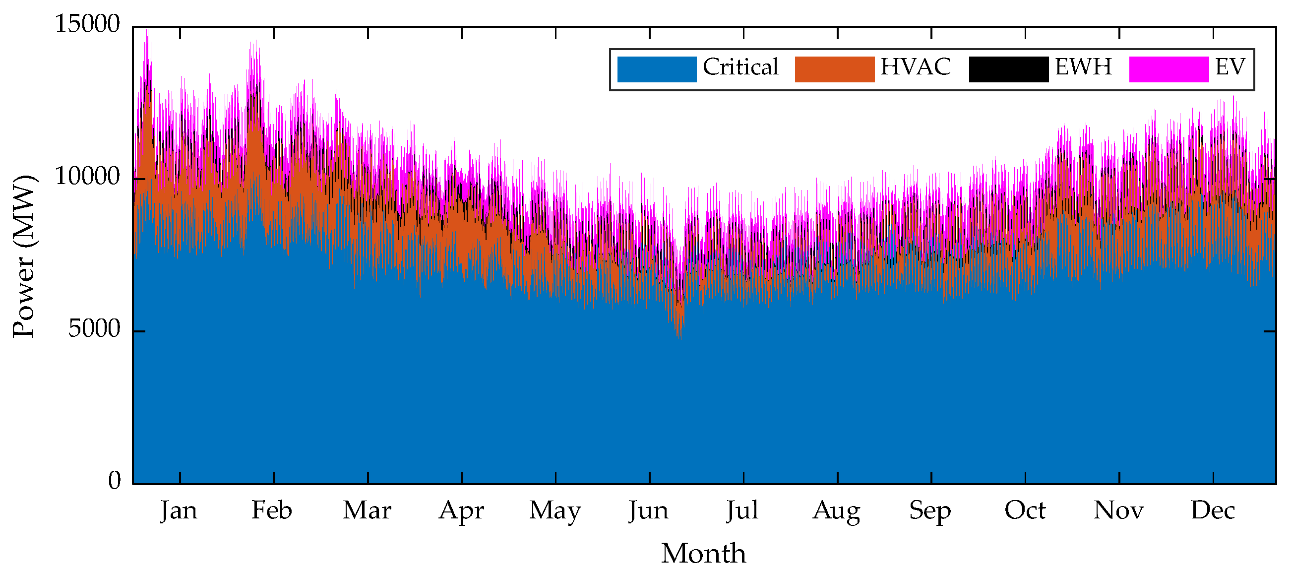
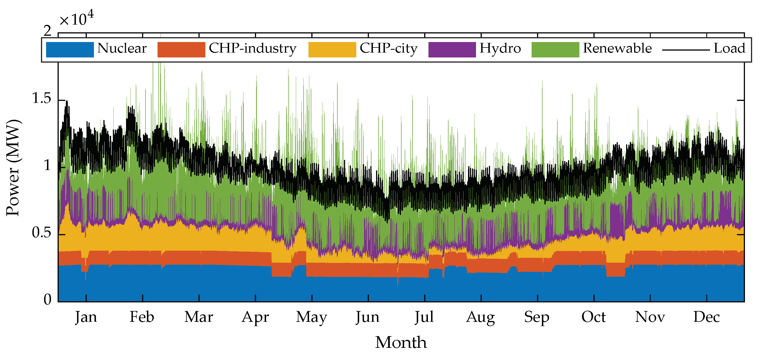
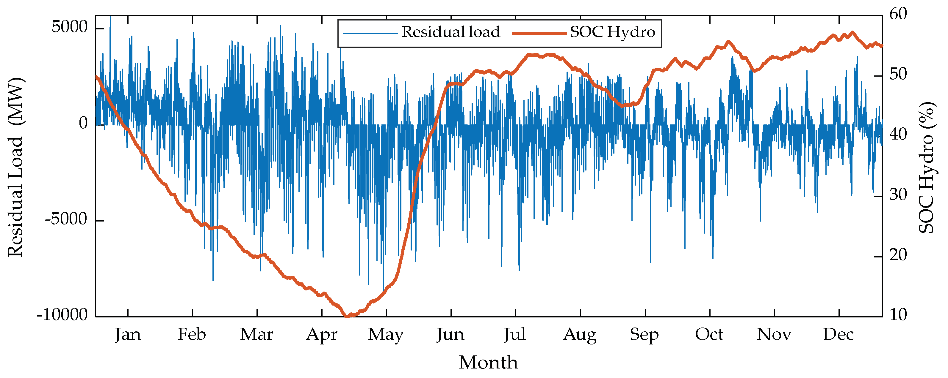
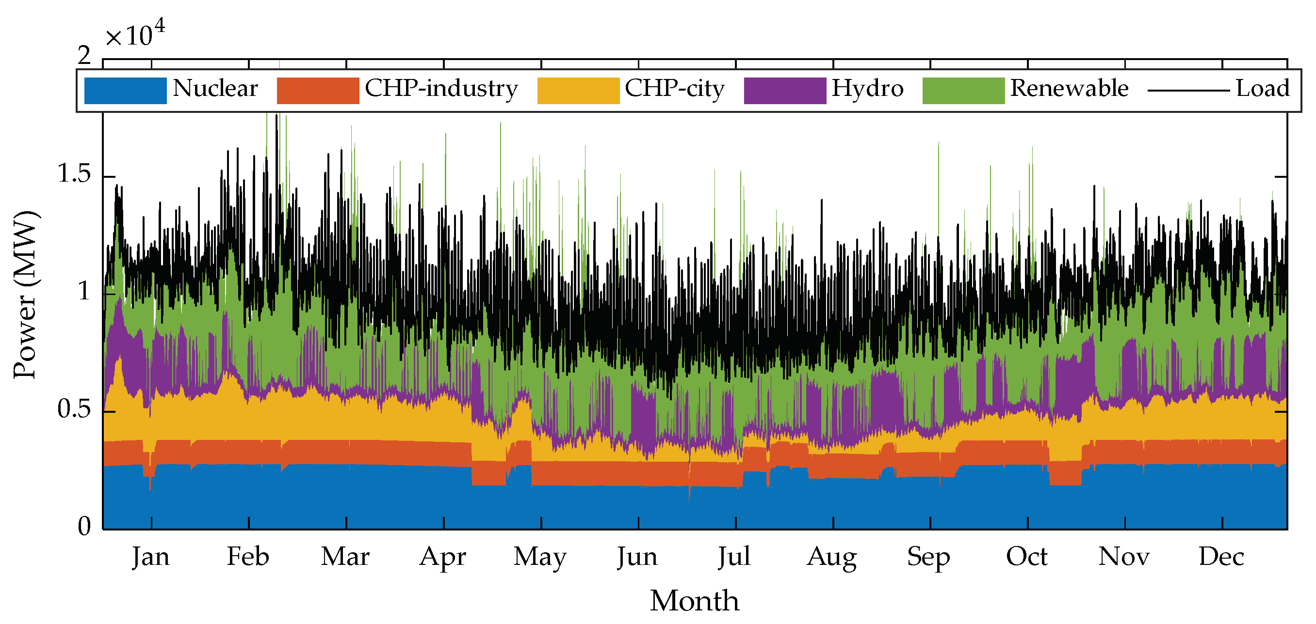
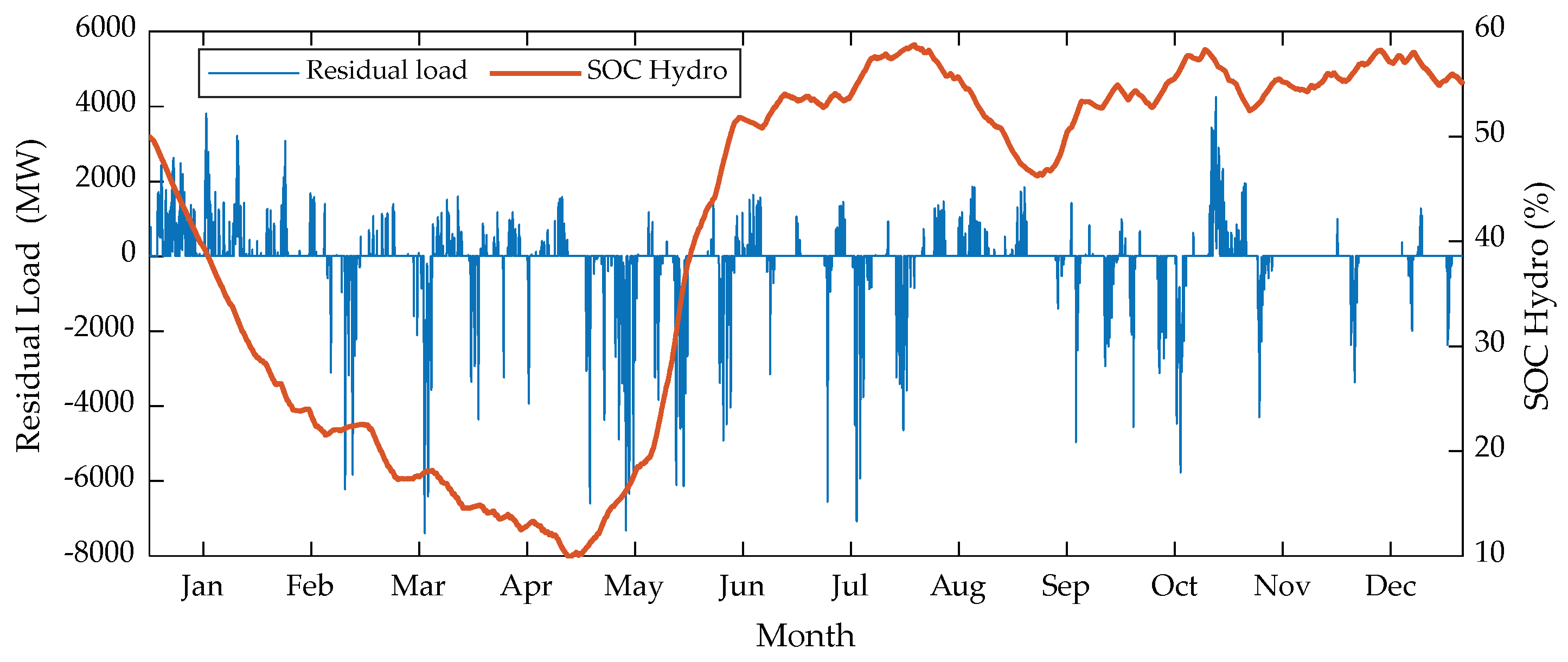
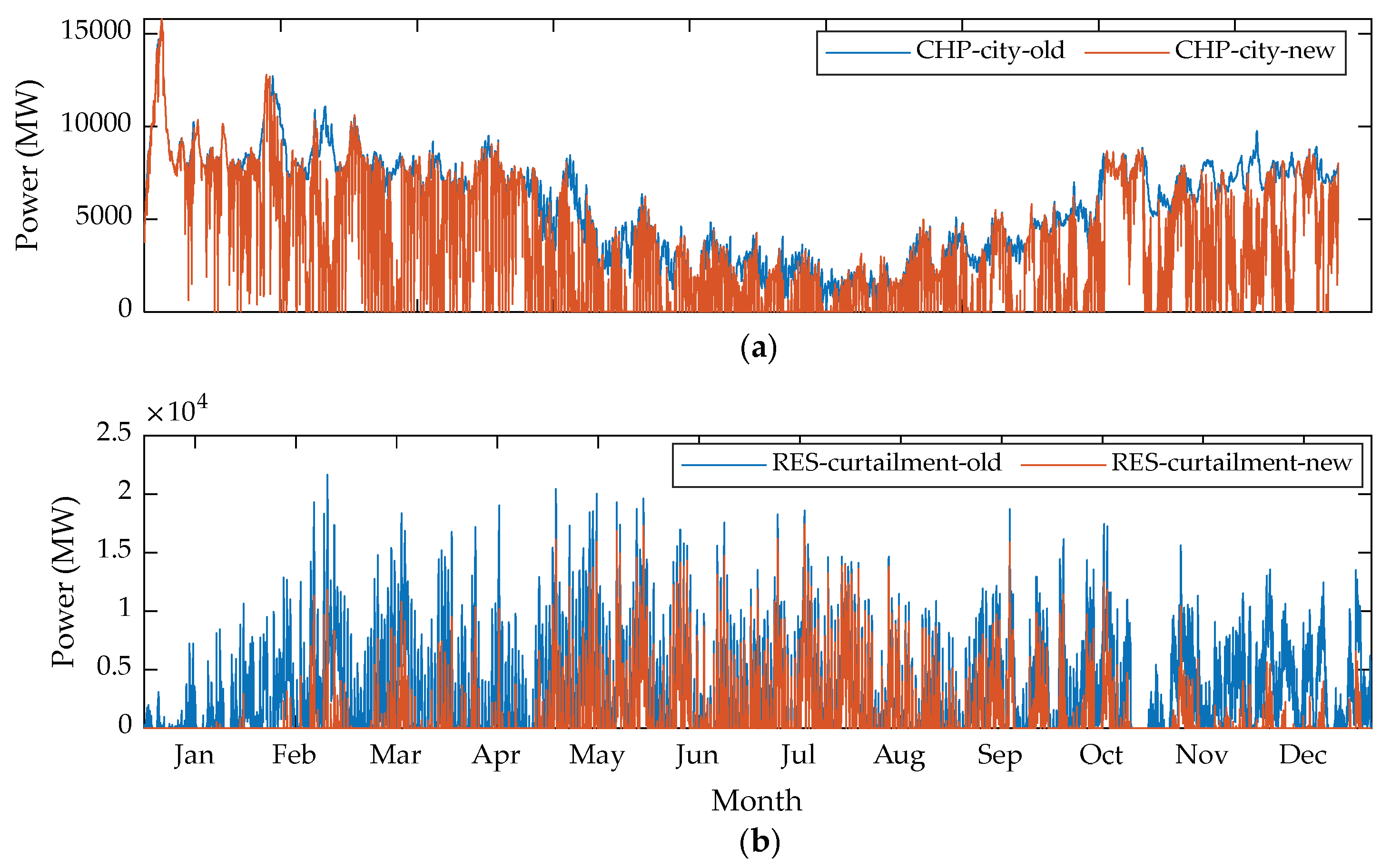
4.2. Simulation Results

The simulated total load and stacked generation profile for Case I are illustrated in Figure 6. Total annual generation was approximately 87 TWh comprising 50% base-load generation, 15% hydro generation, and 35% RESs. This framework resulted in 4.13 TWh of load curtailments and 5.84 TWh of generation curtailments as demonstrated in Figure 7, where positive and negative residual loads implied load curtailment and generation curtailment, respectively. The opposite signs in Figure 7 are used just to differentiate between the two curtailments. Load curtailment represented 4.85% of the total demand, while generation curtailment was 18.89% corresponding to RESs’ penetration. Load curtailment in our simulation implied that this amount of energy had to be met employing conventional power plants that would cause GHG emissions or had to be imported from neighboring countries. Generation curtailment is the amount of RES generation that has to be down regulated in the case there is no demand. The hydro storage operation was very demanding in winter and spring seasons due to high heating demands. The control of hydro-generation alone does not bring substantial benefit to the system.

The load and stacked generation profile, in addition to the residual load balance in Case II are shown in Figure 8 and Figure 9, respectively. The proposed framework showcased a superior performance in Case II, i.e., when residential DR was unleashed. Note that all other loads and generation parameters (except hydro) were the same as in Case I. DR preserves the total flexible demand over the year, i.e., total annual demand remains the same before and after activating DR. However, the hourly demand changes according to the DR framework. When DR was activated, load curtailments were reduced to 0.98 TWh (1.15% of demand), whereas generation curtailment decreased to 1.65 TWh (5.33% of RESs). Compared to Case I, the improvement was 76.2% and 71.7%, respectively. Figure 8 shows how the demand profile tried to match with the RESs closely in Case II, while Figure 9 captures the unserved load and hydro storage variation around the year. The high oscillations in total demand can be seen in Figure 8, which illustrates the effectiveness of the model. Notably, due to high shares of HVAC load in the residential sector, the building thermal inertia and domestic thermal storage together significantly contributed to balance the variations in RESs. The total amount of hydro generation remained almost unchanged but the distribution of the resources around the year was significantly modified and noticeable by comparing Figure 6 and Figure 8.

The simulation results discussed so for are summarized in

Table 1. Results considering one scenario of renewable energy sources (RESs).

Case Study	Load Curtailment (TWh)	RES Curtailment (TWh)
Case I	4.13	5.84
Case II	0.98	1.65

below.

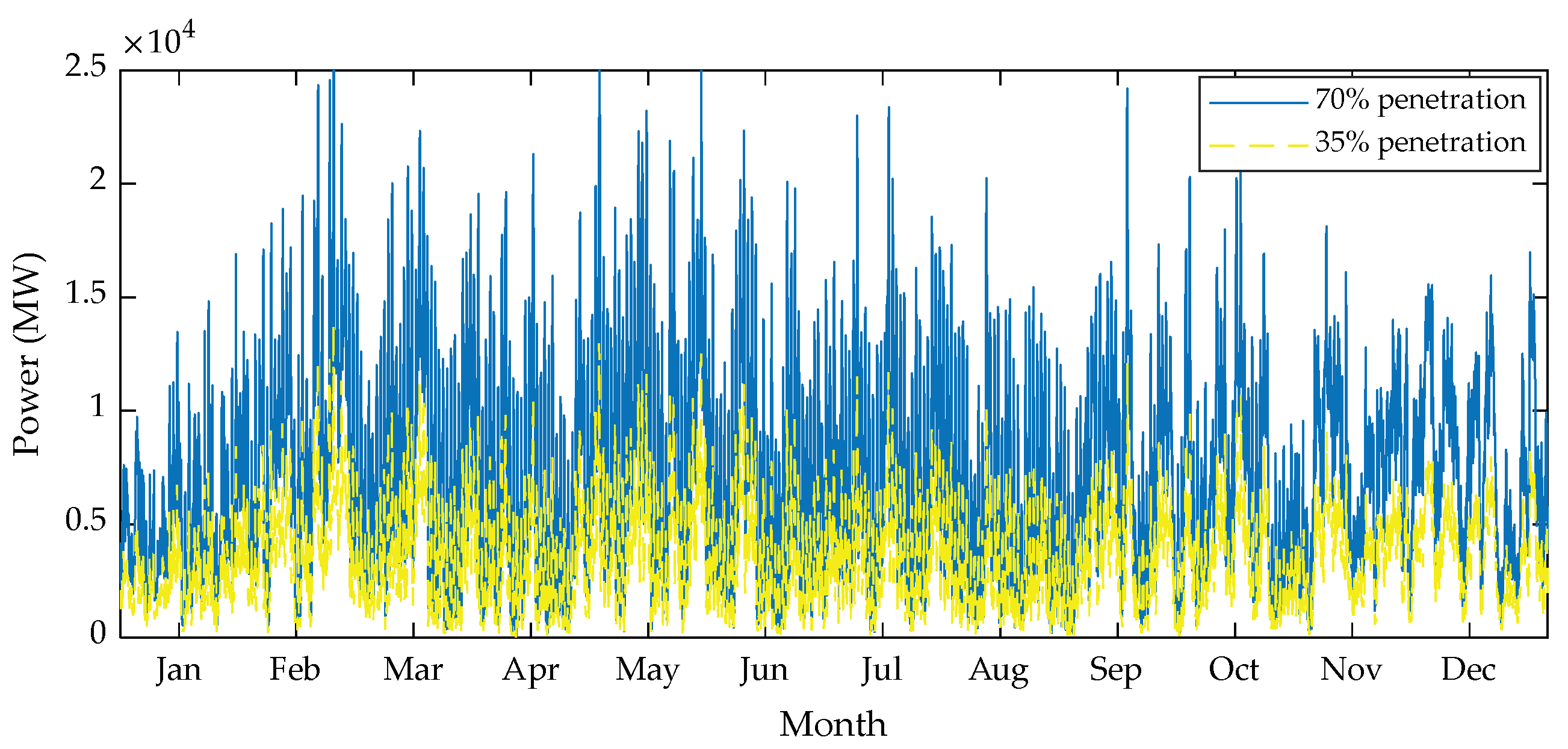
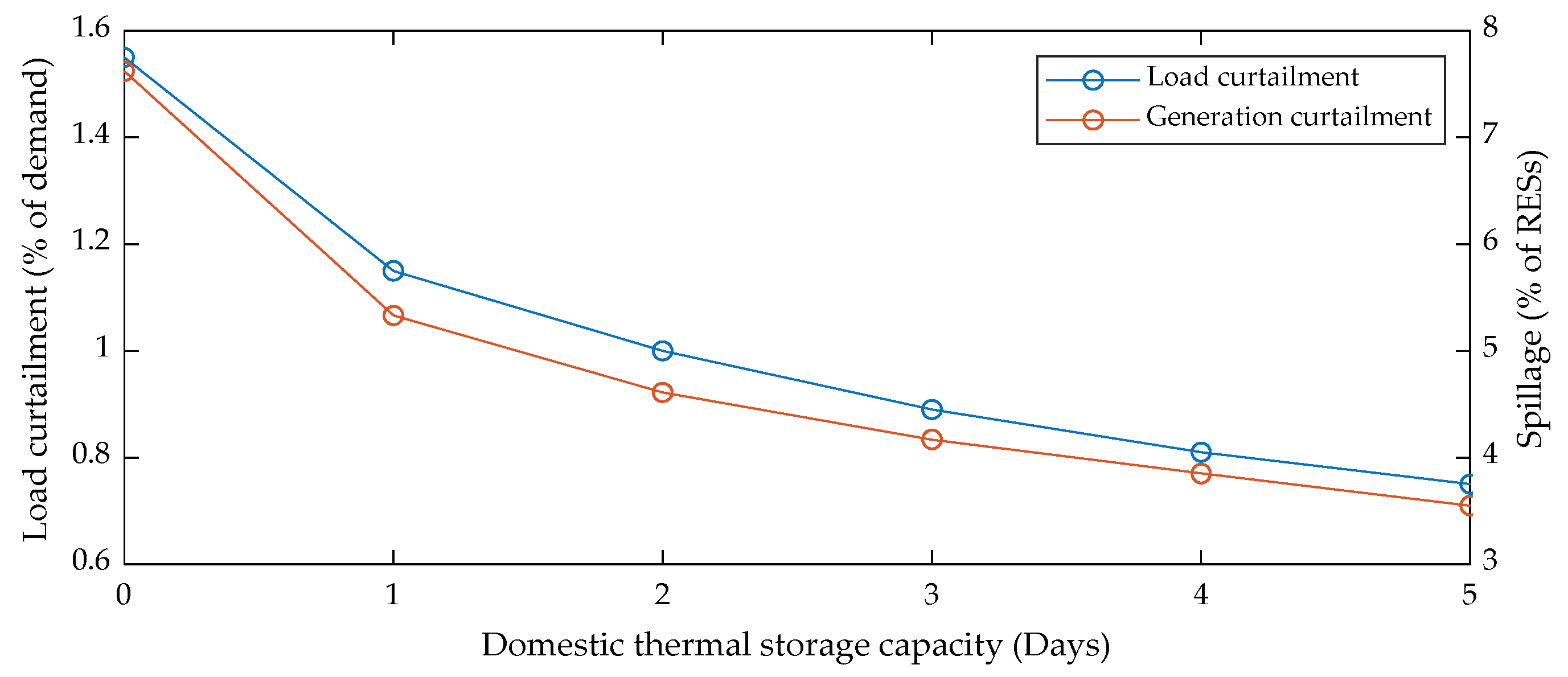
4.3. Sensitivity Analyses

The simulation results presented so far were obtained using one possible scenario (see Figure 4) out of 100 simulated power series of RESs. It was therefore necessary to validate our results against the uncertainty and inherent variability associated with RESs. To do so, the proposed framework was simulated for 100 possible scenarios of RESs. The results thus obtained were analyzed and compared using statistical measures. The purpose was to determine the 95% confidence interval for load and RES curtailments. The summary of the obtained results is given under

Table 2. Statistics of Results with RESs’ Uncertainty.

Case Study	Curtailment	Mean Value (TWh)	Standard Deviation (TWh)	Lower 95% Confidence Bound (TWh)	Upper 95% Confidence Bound (TWh)
Case I	Load	3.748	0.267	3.695	3.8
	Generation	5.168	0.277	5.113	5.222
Case II	Load	0.653	0.19	0.6078	0.698
	Generation	1.112	0.274	1.047	1.177

. The curtailments in Table 1 are comparatively higher than the mean values obtained in Table 2 since the former results were based on a single RESs scenario with a good hourly average.

The effect of varying DR through domestic thermal storage capacity on the decision variables was assessed and the results are illustrated in Figure 10. The Figure clearly shows the affirmative impact of considering thermal storage with 50% of the detached households. Load curtailments were reduced from 1.55% to 1.15% when a storage capacity equal to the heat demand of one day was introduced into the model. The curtailments further dropped to about 1% of total demand when storage capacity increased to two days. Similar behavior was visible for RES curtailment. RES curtailment decreased drastically when thermal storage of one-day capacity was integrated. The improvement was significant only until storage capacity of 2 days, after which, the benefit was marginal.

Lastly, the impact of increasing RES penetration on curtailment levels was analyzed and the results are listed in

Table 3. Effect of Increasing RES Penetration.

RES Penetration (%)	Aggregated Generation as % of Total Demand	Case I		Case II
		Load Curtailment (TWh)	RES Curtailment (TWh)	Load Curtailment (TWh)	RES Curtailment (TWh)
35	102.1	4.130	5.84	0.982	1.65
40	107.23	3.215	9.339	0.484	4.921
45	112.41	2.586	13.128	0.320	8.456
50	117.6	2.248	17.207	0.227	12.538
55	122.8	1.974	21.351	0.176	16.790
60	127.98	1.752	25.546	0.143	21.082
65	133.15	1.566	29.777	0.117	25.419
70	138.34	1.409	34.038	0.095	29.781

. Please note that base-load generation was in the same place. Evidently, the higher penetrations reduced load curtailments but on the contrary, increased RES curtailments due to excessive generation in the system. The effect of coordinating DR with hydro-storage, i.e., Case II, on curtailments was visible from the results at all penetration levels. From Load curtailment reduction perspective, the benefit in case II increased with higher penetrations compared to Case I. The relative benefit was 76.2% at 35% RES penetration, which increased to 92% at 70% RES penetration. However, the results for RES curtailments were the opposite as the relative benefit in Case II decreased to 12.5% at 70% penetration level. This was due to the thermal and load constraints aimed to preserve the comfort levels and total demand of households over the year. DR was subdued by such constraints.

Excess RESs production at higher penetration levels summarized in Table 3 should be utilized effectively to prevent down regulation. One possible solution is aimed to partially replace heat and electricity production of CHP-city with surplus RESs, since CHP-city contributes to carbon emissions. For instance, using the electricity to heat ratio, 1.31 MW of surplus RESs would imply 0.31 MW reduction in electrical output, while 1 MW reduction in heat generation of CHP-city. This way, a considerable number of district heated buildings in Finland can shift to electrical loads, e.g., ground source heat pump or direct electrical heating. The proposed option was simulated for Case II and the decline in CHP-city production (heat + electrical), after being replaced with surplus RES, is analyzed in

Table 4. Effect of Replacing CHP-city Production with Surplus RESs in Case II.

RES Penetration (%)	RES Curtailment (TWh)	Reduction in Curtailment (%)	CHP-city Electricity Production (TWh)	CHP-city Heating Production (TWh)	CHP-city Total Production (TWh)
35	0.174	89.45	11.628	37.51	49.14
40	0.67	86.38	10.970	35.39	46.36
45	1.424	83.16	10.313	33.27	43.58
50	2.510	79.98	9.603	30.98	40.58
55	3.885	76.86	8.923	28.785	37.71
60	5.617	73.35	8.318	26.832	35.15
65	7.445	70.71	7.724	24.916	32.64
70	9.644	67.62	7.212	23.265	30.48

. It was assumed as direct electrical heat in this case. Note that the initial total CHP annual production was 50.6 TWh, i.e., 11.97 TWh (14% of total) electricity and 38.6 TWh heat. At 35% penetration, 89.45% of surplus RESs in Case II were utilized compared to the results in Table 3. The utilization advantage remains prominent even at higher penetrations and this effectively brings down the emissions of CHP-city. The difference between the results is illustrated in Figure 11 for 70% RES penetration. It is to be noted that this solution did not result in considerable amount of curtailment reductions during the summer season. The reason is that RES (both wind and solar) production was extremely higher, and residential demand was less. CHP production was also smaller as it mainly followed the external temperature variation. Furthermore, the proposed solution would require high ramp-up and ramp-down rates, which is definitely possible for CHP-city.

5. Conclusions

Curtailment events are usually inevitable when RESs are deployed at a large scale. Such events are discouraging for system stakeholders. This paper proposes a mathematical framework to demonstrate how aggregated hydro-storage in conjunction with residential DR loads can provide balancing services in a highly renewable generation based power system. Adequate modeling for each system component was considered in our study. The proposed framework was applied to a Finnish case study with different RES penetrations. Results prove that unleashing DR by system operators can effectively mitigate the curtailments that would be translated into the operating cost of power systems. The presented study showed the possible option of mitigating the load and RES curtailments against very high RES penetration that is needed for carbon free energy systems in Finland. RES spillage at very high penetrations can be avoided by replacing the CHP-city production in proportion to the electricity to heat ratio. High RES penetration would contribute to GHG emission reduction significantly while resulting into economical benefits such as reduction in electricity spot price. The supply curve in spot market is based on the marginal prices of each generating unit. The generation bids are arranged in the ascending order with respect to the offered price. The cheapest generation is dispatched first. In this way, RES generators will clear the market most of the time.

References

1. European Commission: Climate and Energy Framework. Available online: https://ec.europa.eu/clima/policies/strategies/2030_en (accessed on 1 December 2018).
2. Bird, L.; Lew, D.; Milligan, M.; Carlini, E.M.; Estanqueiro, A.; Flynn, D.; Gomez-Lazaro, E.; Holttinen, H.; Menemenlis, N.; Orths, A.; et al. Wind and solar energy curtailment: A review of international experience. Renew. Sustain. Energy Rev. 2016, 65, 577–586. [Google Scholar] [CrossRef]
3. Zakeri, B.; Syri, S. Economy of electricity storage in the Nordic electricity market: The case for Finland. In Proceedings of the 11th International Conference on the European Energy Market (EEM14), Krakow, Poland, 28–30 May 2014; pp. 1–6. [Google Scholar]
4. Safdarian, A.; Ali, M.; Fotuhi-Firuzabad, M.; Lehtonen, M. Domestic EWH and HVAC management in smart grids: Potential benefits and realization. Electr. Power Syst. Res. 2016, 134, 38–46. [Google Scholar] [CrossRef] [Green Version]
5. Ali, M.; Humayun, M.; Degefa, M.; Alahäivälä, A.; Lehtonen, M.; Safdarian, A. A framework for activating residential HVAC demand response for wind generation balancing. In Proceedings of the 2015 IEEE Innovative Smart Grid Technologies—Asia (ISGT ASIA), Bangkok, Thailand, 3–6 November 2015; pp. 1–6. [Google Scholar] [CrossRef]
6. Bashir, A.; Pourakbari Kasmaei, M.; Safdarian, A.; Lehtonen, M. Matching of Local Load with On-Site PV Production in a Grid-Connected Residential Building. Energies 2018, 11, 2409. [Google Scholar] [CrossRef]
7. Nguyen, D.T.; Le, L.B. Joint Optimization of Electric Vehicle and Home Energy Scheduling Considering User Comfort Preference. IEEE Trans. Smart Grid 2014, 5, 188–199. [Google Scholar] [CrossRef]
8. Safdarian, A.; Fotuhi-Firuzabad, M.; Lehtonen, M. Benefits of Demand Response on Operation of Distribution Networks: A Case Study. IEEE Syst. J. 2016, 10, 189–197. [Google Scholar] [CrossRef]
9. Nguyen, D.T.; Le, L.B. Optimal Bidding Strategy for Microgrids Considering Renewable Energy and Building Thermal Dynamics. IEEE Trans. Smart Grid 2014, 5, 1608–1620. [Google Scholar] [CrossRef]
10. Bashir, A.A.; Lehtonen, M. Day-Ahead Rolling Window Optimization of Islanded Microgrid with Uncertainty. In Proceedings of the 2018 IEEE PES Innovative Smart Grid Technologies Conference Europe (ISGT-Europe), Sarajevo, Bosnia-Herzegovina, 21–25 October 2018; pp. 1–6. [Google Scholar]
11. Ali, M.; Ekstrom, J.; Alahaivala, A.; Lehtonen, M. Assessing the upward demand response potential for mitigating the wind generation curtailment: A case study. In Proceedings of the 2017 14th International Conference on the European Energy Market (EEM), Dresden, Germany, 6–9 June 2017; pp. 1–6. [Google Scholar]
12. Ali, M.; Humayun, M.; Degefa, M.; Lehtonen, M.; Safdarain, A. Optimal DR through HVAC loads in distribution systems hosting large wind generation. In Proceedings of the 2015 IEEE Innovative Smart Grid Technologies—Asia (ISGT ASIA), Bangkok, Thailand, 3–6 November 2015; pp. 1–6. [Google Scholar]
13. Ali, M.; Ekström, J.; Lehtonen, M. Sizing Hydrogen Energy Storage in Consideration of Demand Response in Highly Renewable Generation Power Systems. Energies 2018, 11, 1113. [Google Scholar] [CrossRef]
14. Ali, M.; Ekström, J.; Lehtonen, M. Assessing the Potential Benefits and Limits of Electric Storage Heaters for Wind Curtailment Mitigation: A Finnish Case Study. Sustainability 2017, 9, 836. [Google Scholar] [CrossRef]
15. Chen, X.; Kang, C.; O’Malley, M.; Xia, Q.; Bai, J.; Liu, C.; Sun, R.; Wang, W.; Li, H. Increasing the Flexibility of Combined Heat and Power for Wind Power Integration in China: Modeling and Implications. IEEE Trans. Power Syst. 2015, 30, 1848–1857. [Google Scholar] [CrossRef]
16. Grünewald, P.; McKenna, E.; Thomson, M. Going with the wind: Temporal characteristics of potential wind curtailment in Ireland in 2020 and opportunities for demand response. IET Renew. Power Gener. 2015, 9, 66–77. [Google Scholar] [CrossRef]
17. Fingrid Finland. Available online: www.fingrid.fi (accessed on 1 December 2018).
18. Statistics Finland. Available online: www.stat.fi (accessed on 15 December 2018).
19. Nord-Pool. Available online: www.nordpoolspot.com (accessed on 1 December 2018).
20. Ekström, J.; Koivisto, M.; Mellin, I.; Millar, J.; Saarijärvi, E.; Haarla, L. Assessment of large scale wind power generation with new generation locations without measurement data. Renew. Energy 2015, 83, 362–374. [Google Scholar] [CrossRef]
21. Ekström, J.; Koivisto, M.; Millar, J.; Mellin, I.; Lehtonen, M. A statistical approach for hourly photovoltaic power generation modeling with generation locations without measured data. Sol. Energy 2016, 132, 173–187. [Google Scholar] [CrossRef]
22. Ali, M.; Safdarian, A.; Lehtonen, M. Demand response potential of residential HVAC loads considering users preferences. In Proceedings of the IEEE PES Innovative Smart Grid Technologies, Europe, Istanbul, Turkey, 12–15 October 2014; pp. 1–6. [Google Scholar]
23. Finnish National Travel Survey. Available online: www.vayla.fi (accessed on 30 October 2018).
24. Alahäivälä, A.; Saarijärvi, E.; Lehtonen, M. Modeling Electric Vehicle Charging Flexibility for the Maintaining of Power Balance. Int. Rev. Electr. Eng. 2013, 8, 1759–1769. [Google Scholar]
Figure 1. Daily average inflow to aggregated hydro storage in Finland in 2017.
Energies 12 01037 g001
Figure 2. Two-capacity building thermal model.
Energies 12 01037 g002
Figure 3. Hourly base-load generation profile.
Energies 12 01037 g003
Figure 4. Renewable energy sources (RESs) penetrations (70% wind and 30% solar).
Energies 12 01037 g004
Figure 5. Hourly dis-aggregated demand profile.
Energies 12 01037 g005
Figure 6. Load and generation profile for Case I.
Energies 12 01037 g006
Figure 7. Residual load and hydro-storage dynamics for Case I.
Energies 12 01037 g007
Figure 8. Load and generation profile for Case II.
Energies 12 01037 g008
Figure 9. Residual load and hydro-storage dynamics for Case II.
Energies 12 01037 g009
Figure 10. Effect of varying thermal storage capacity.
Energies 12 01037 g010
Figure 11. CHP–city replaced with surplus RESs (70% penetration) for Case II: (a) CHP production; (b) RESs curtailments.
Energies 12 01037 g011