Design and Implementation of a New Algorithm for Enhancing MPPT Performance in Solar Cells


 ,
,
Abstract
:1. Introduction
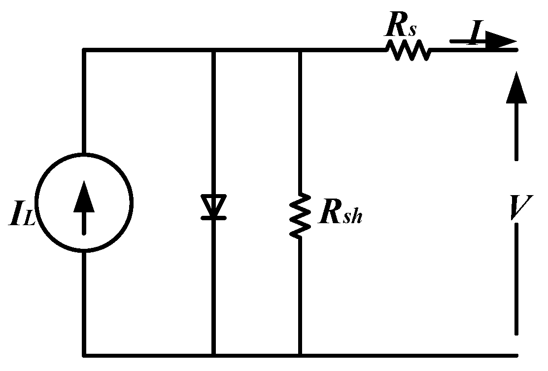
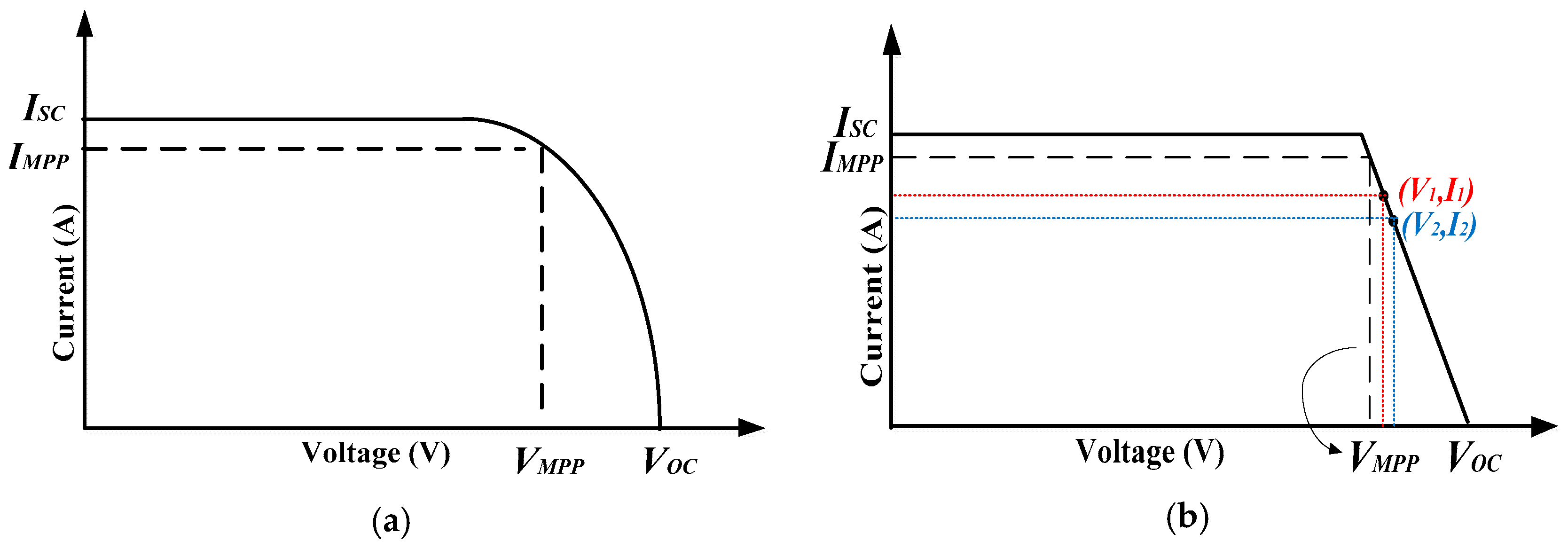
2. Solar Cell
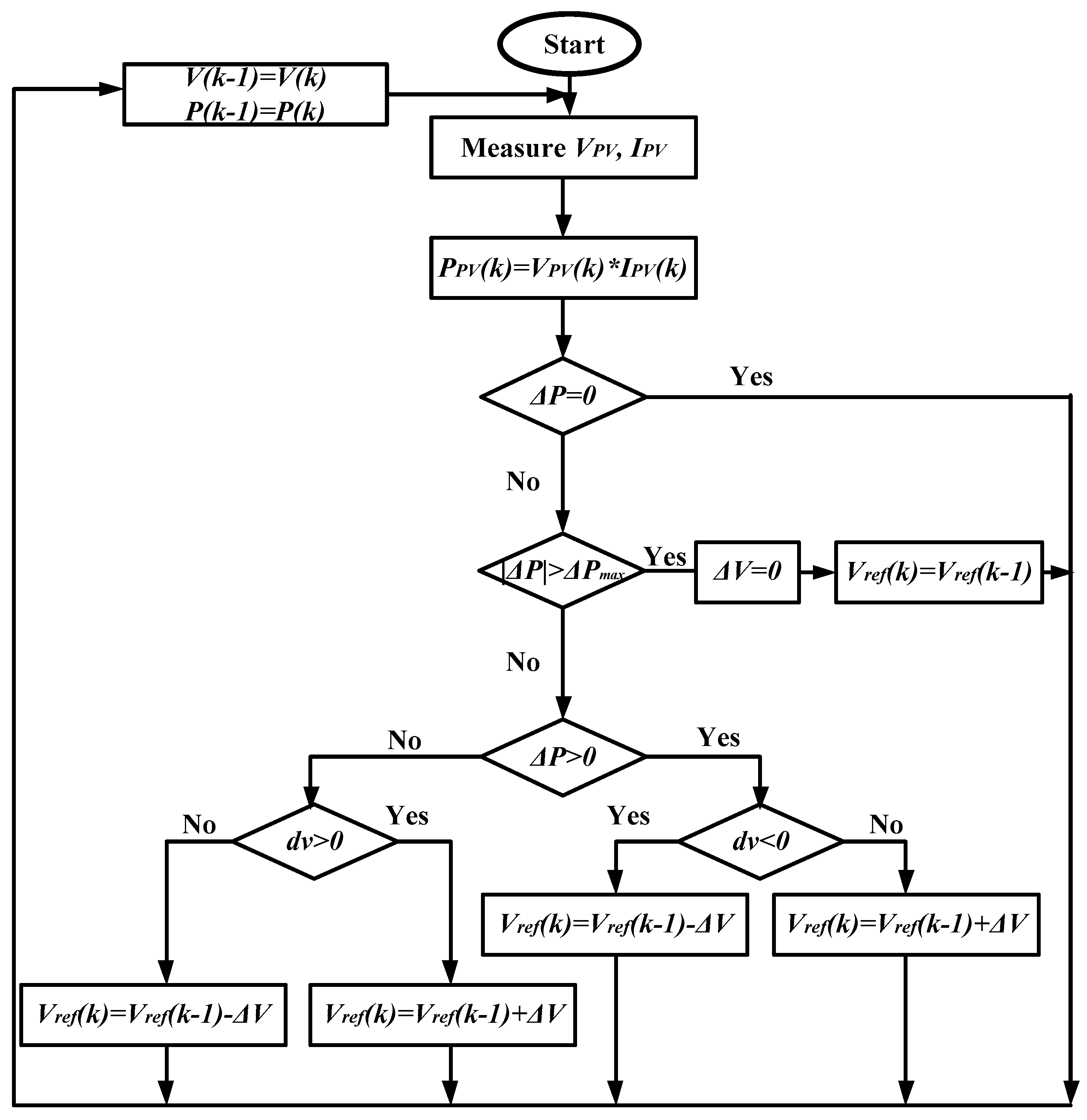
3. Proposed MPPT Algorithm
3.1. CPV Algorithm
3.2. Selection of ΔV
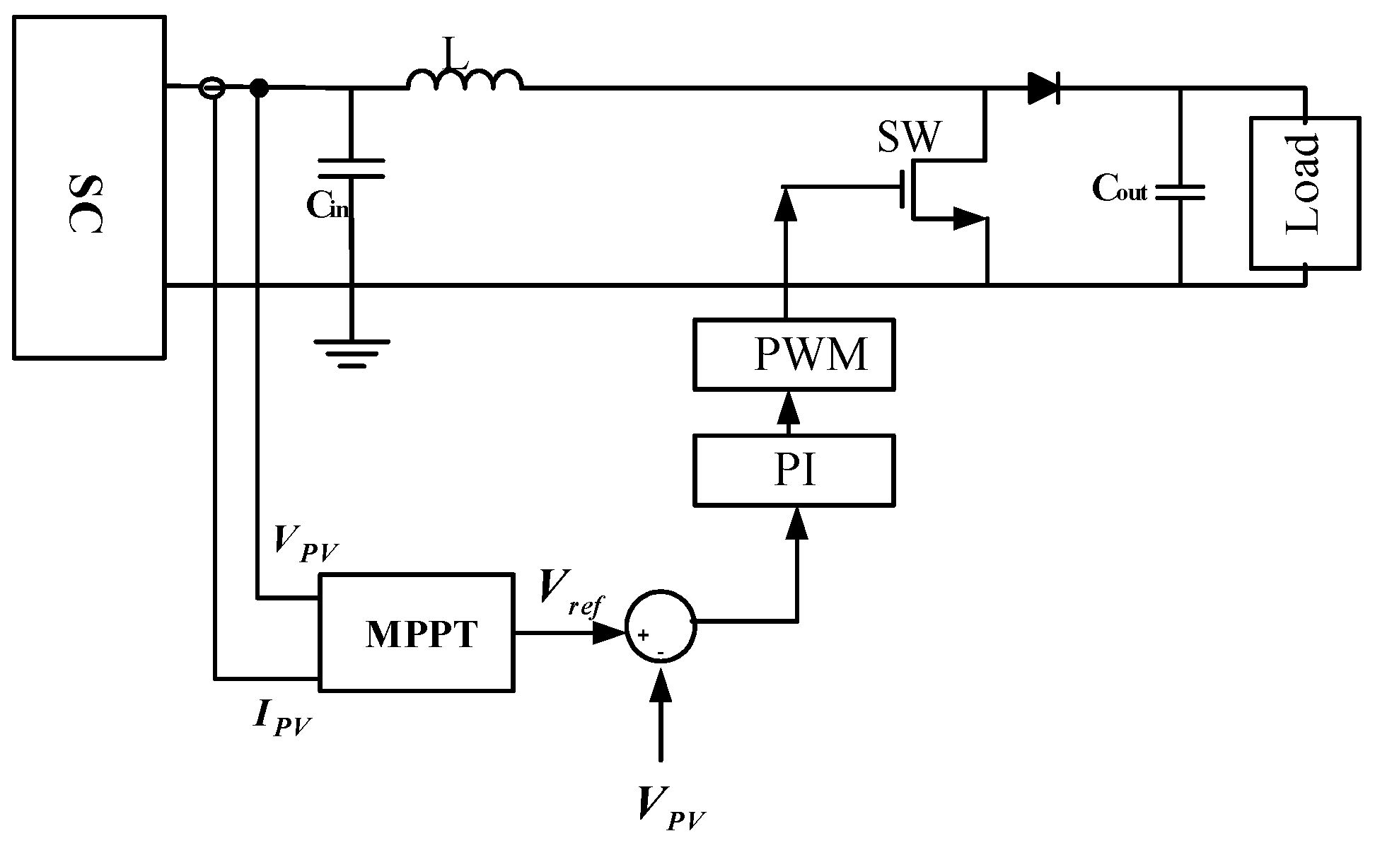
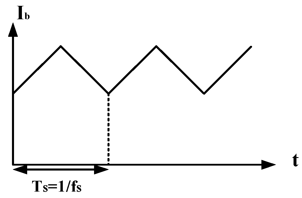
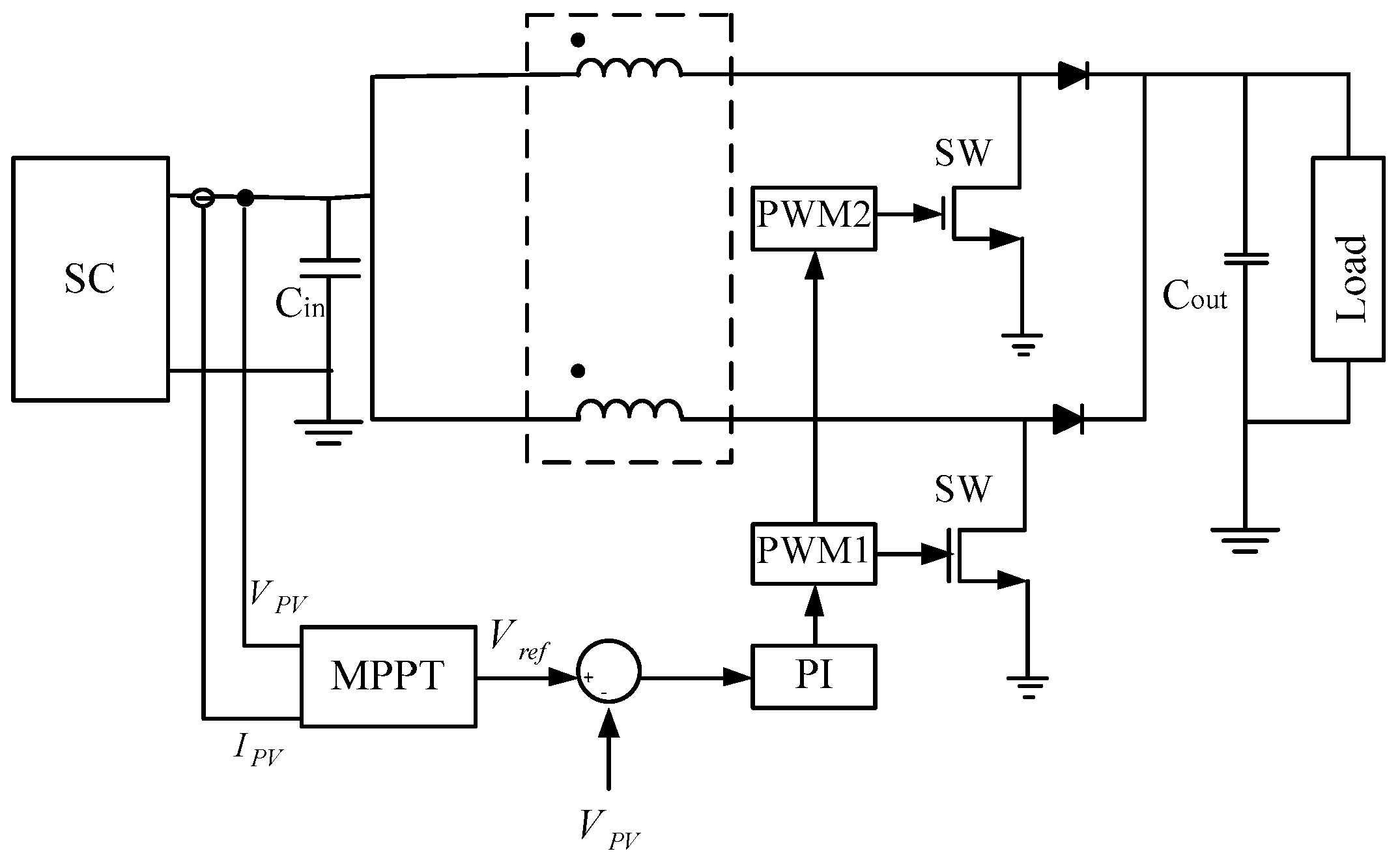
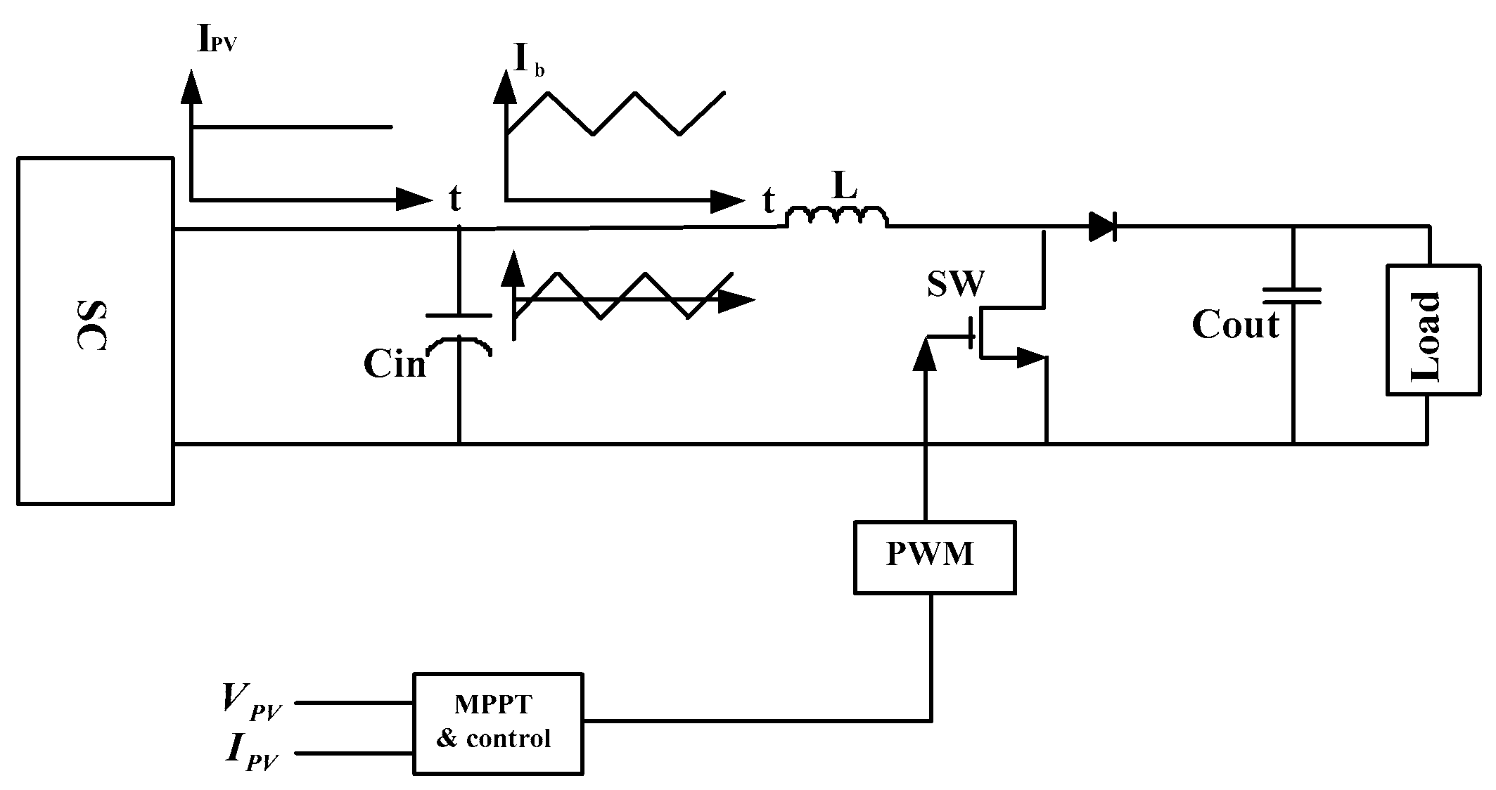
3.3. Boost Converter
4. Analysis of the Simulation and Experimental Results
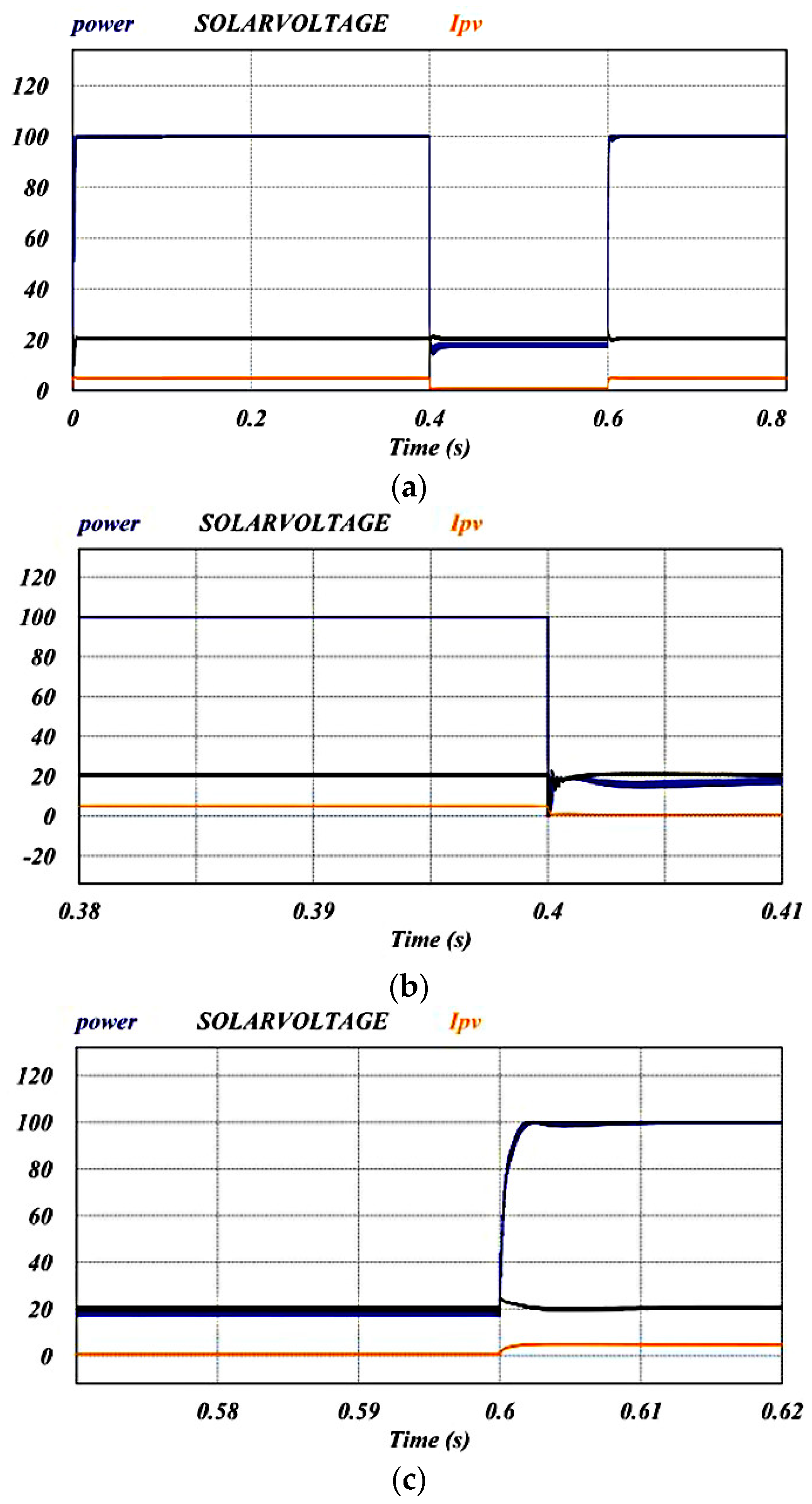
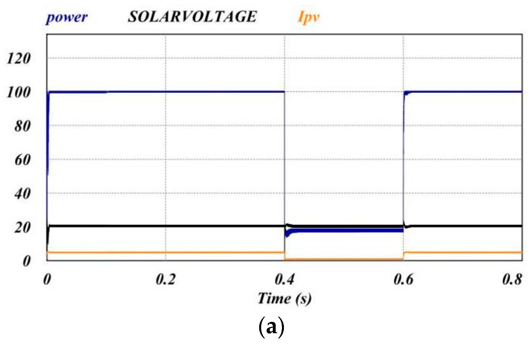
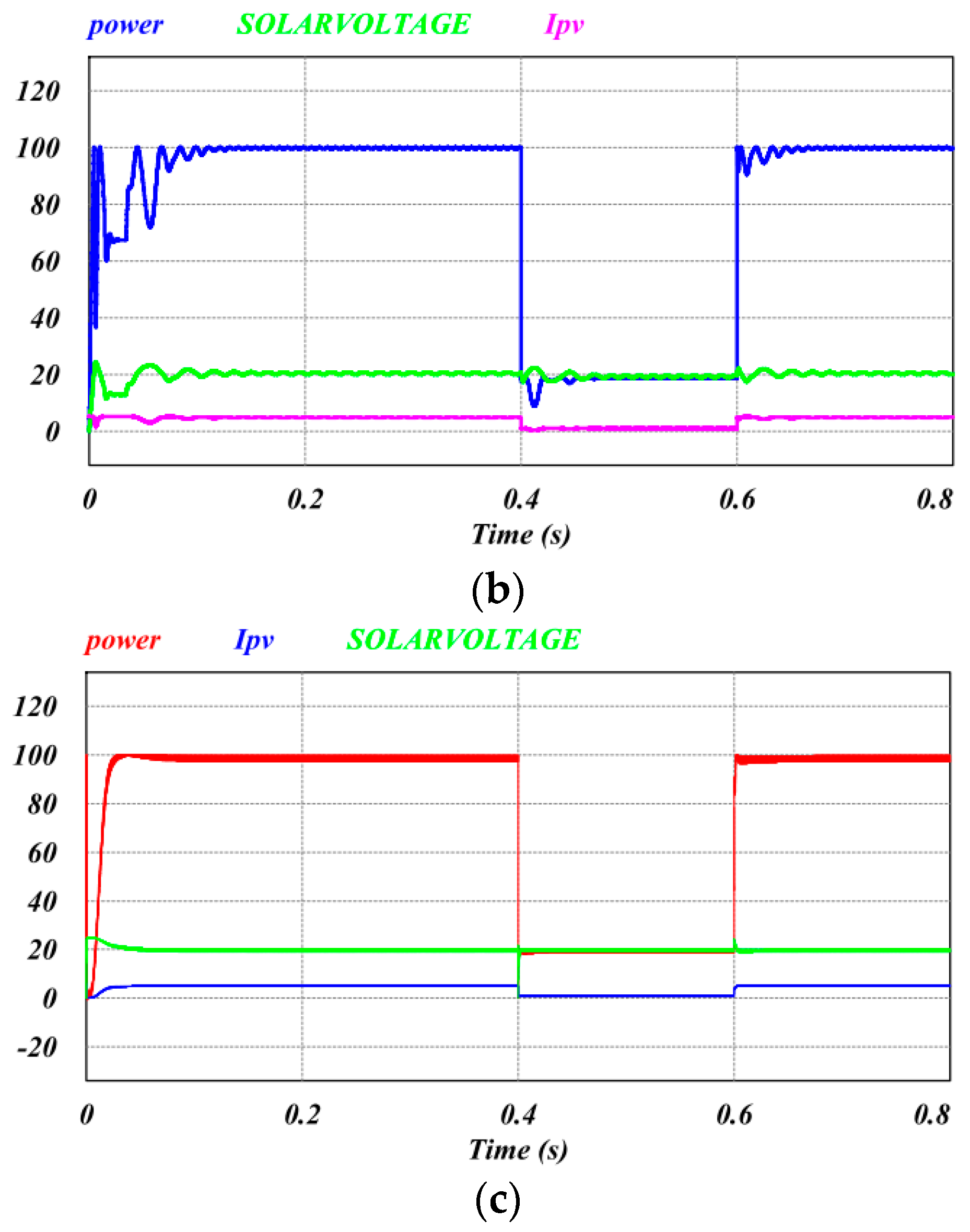
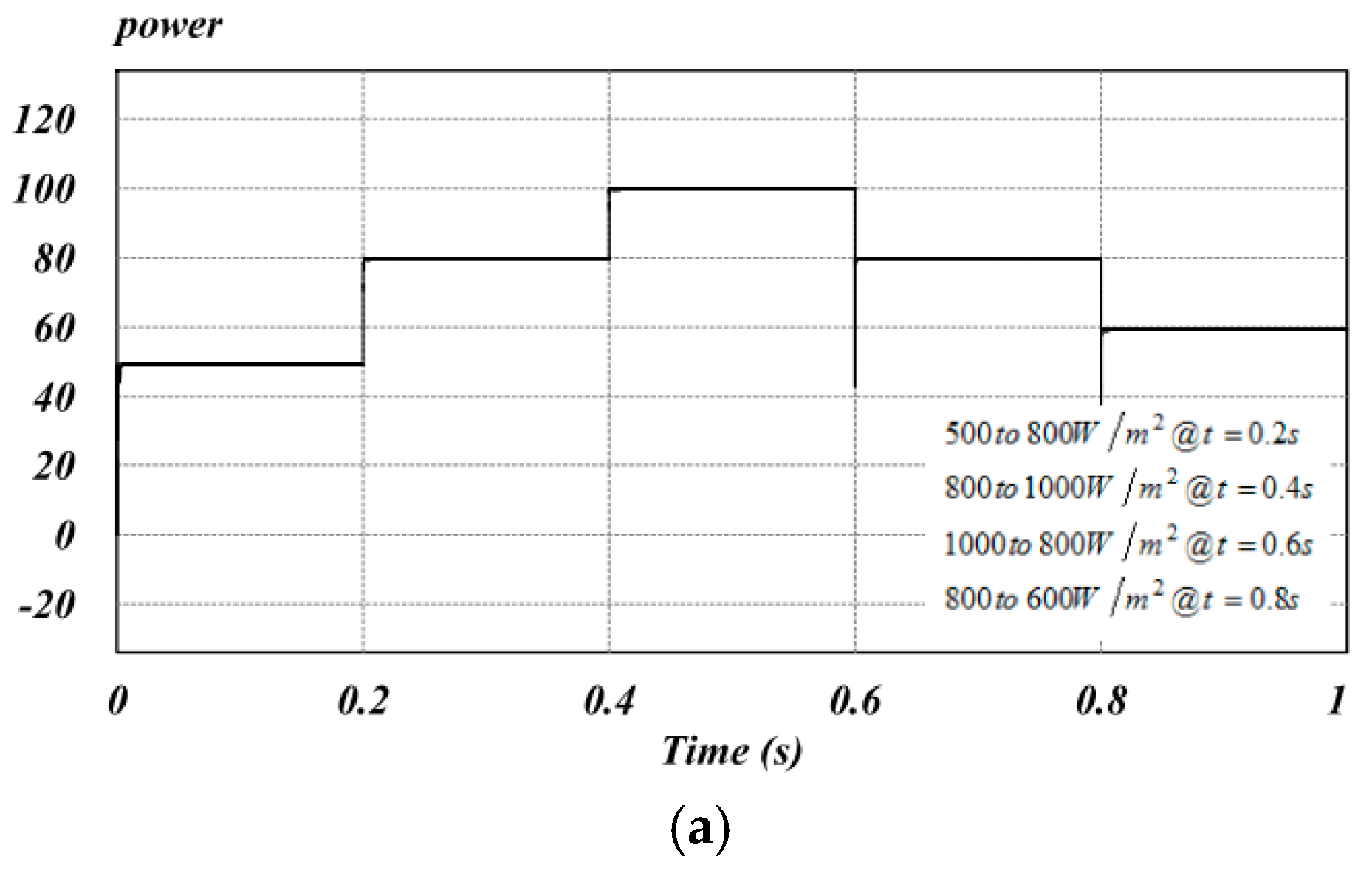
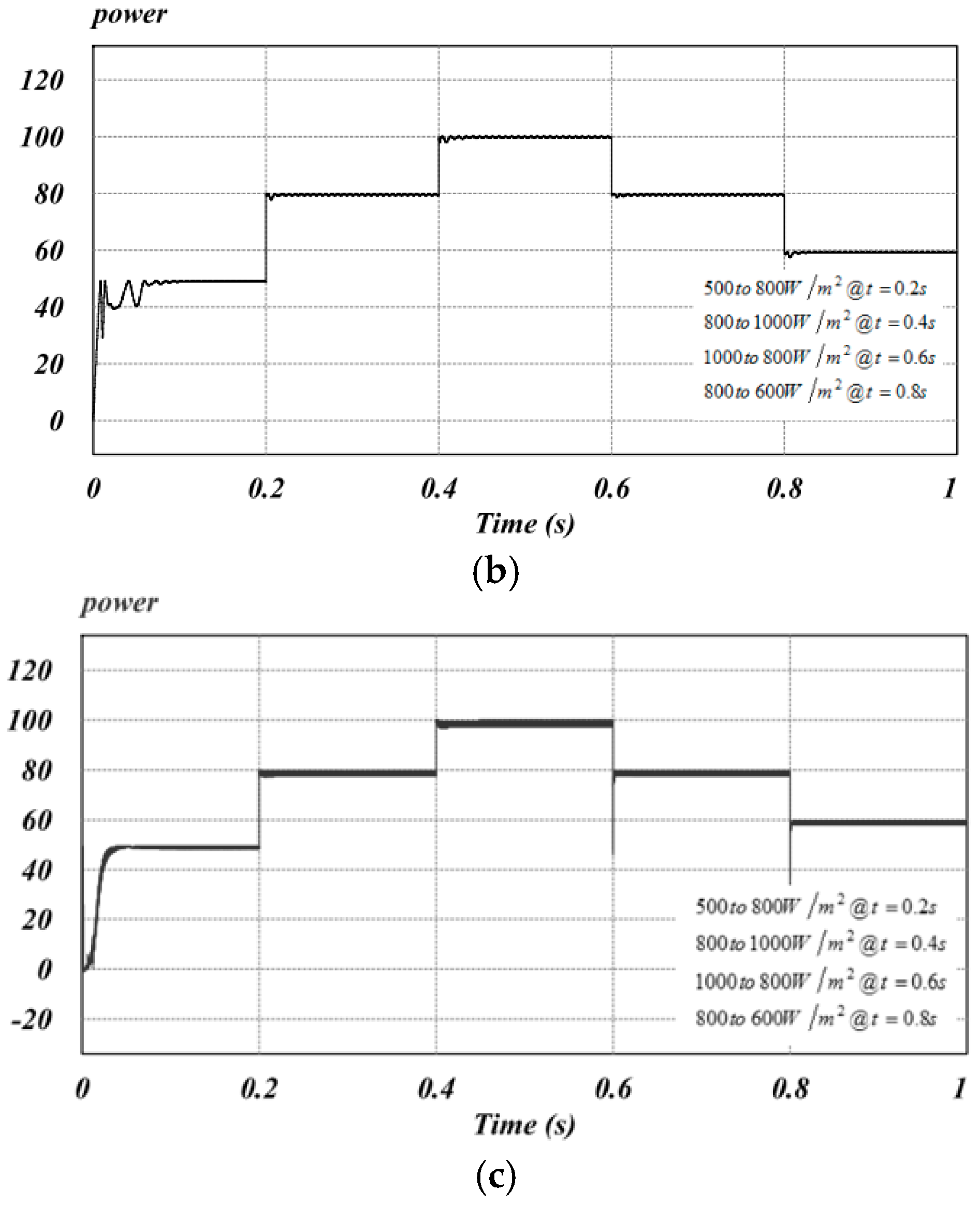
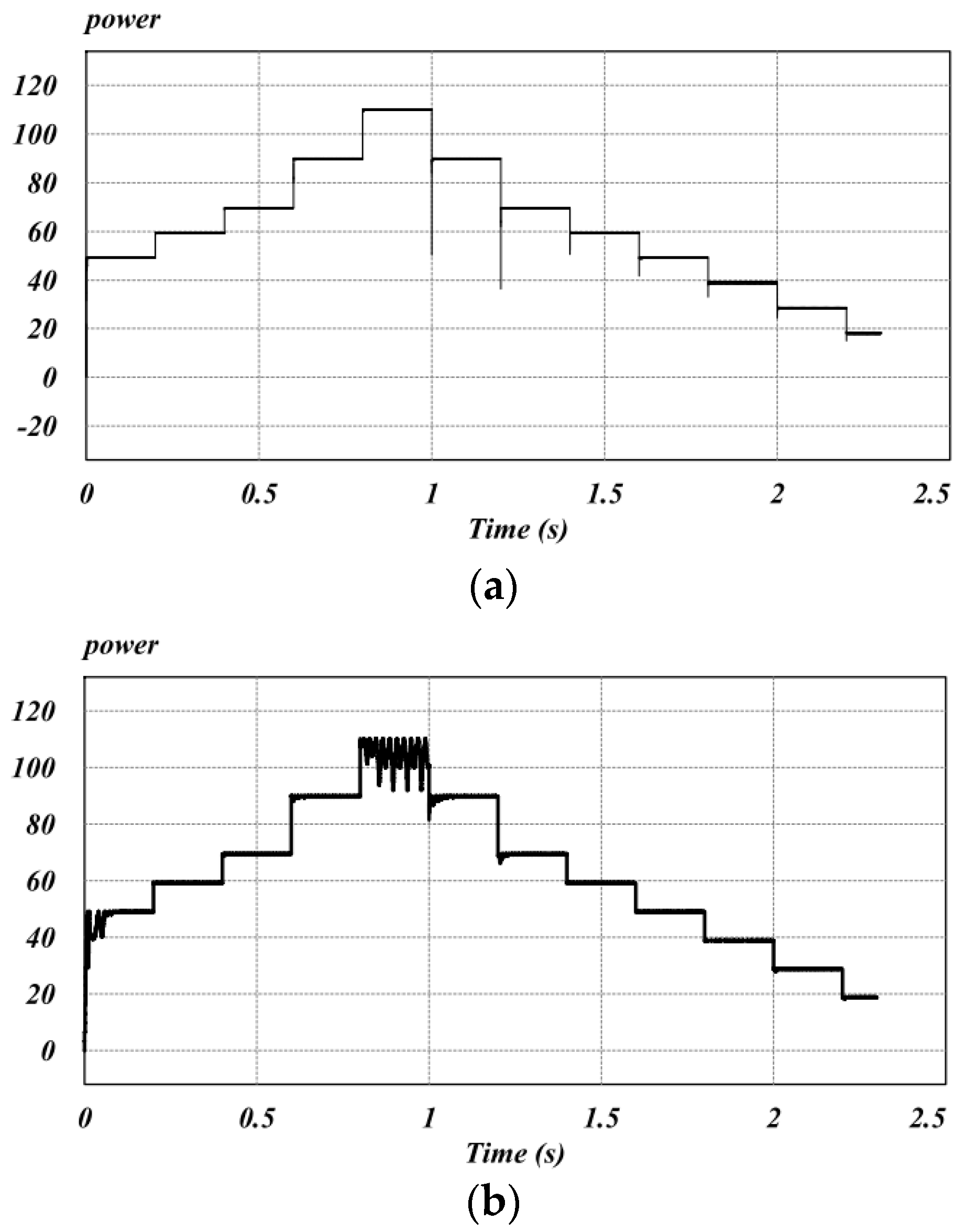
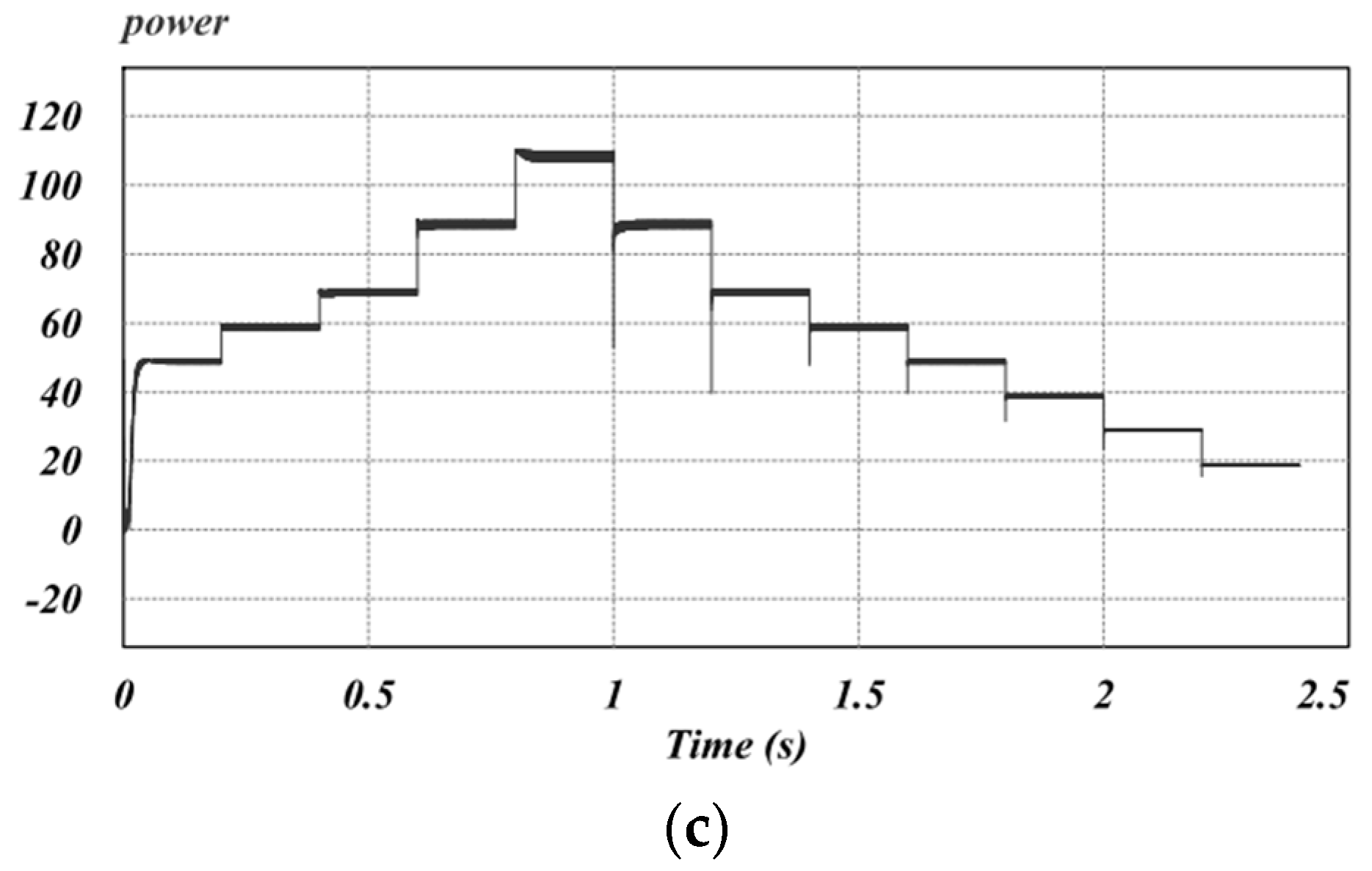
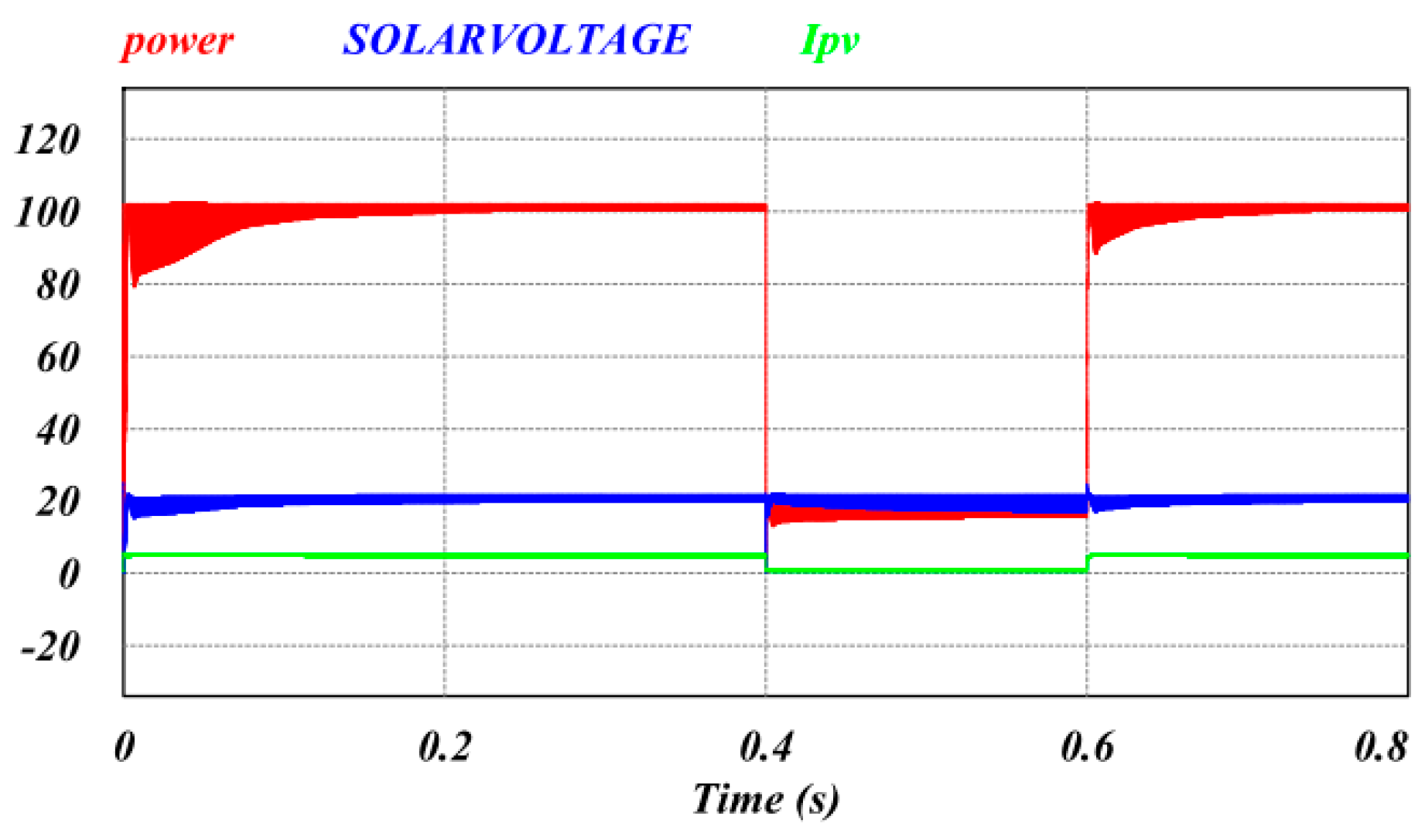
4.1. Simulation Results and Analysis
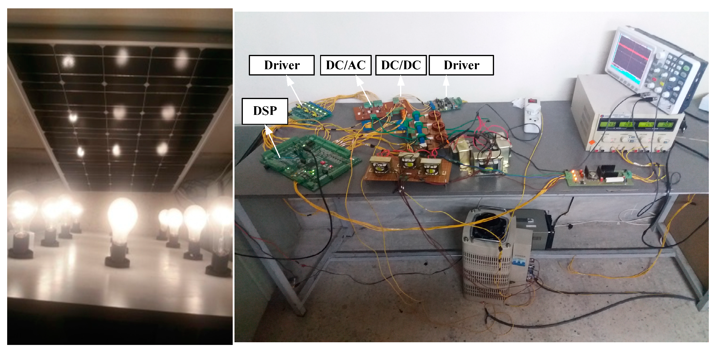
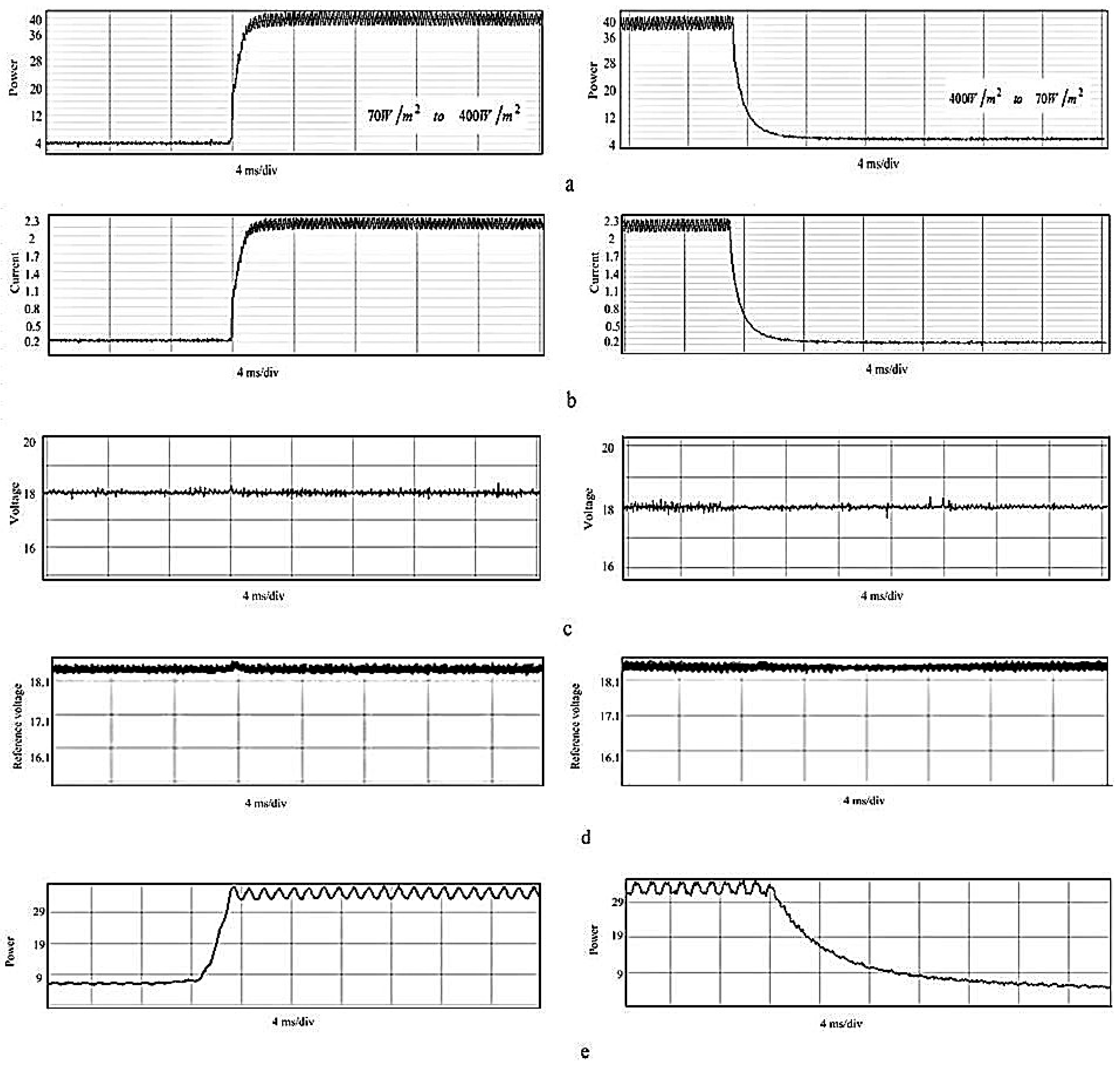
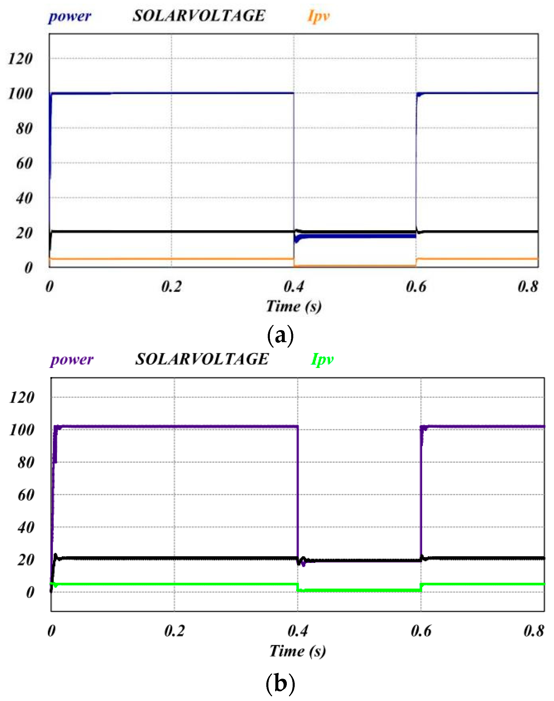
4.2. Experimental Results and Analysis
4.3. Comparative Study
5. Conclusions
Author Contributions
Funding
Conflicts of Interest
References
- Rahmanian, E.; Akbari, H.; Sheisi, G.H. Maximum power point tracking in grid connected wind plant by using intelligent controller and switched reluctance generator. IEEE Trans. Sustain. Energy 2017, 8, 1313–1320. [Google Scholar] [CrossRef]
- De Brito, M.A.G.; Galotto, L.; Sampaio, L.P.; e Melo, G.D.A.; Canesin, C.A. Evaluation of the main mppt techniques for photovoltaic applications. IEEE Trans. Ind. Electron. 2013, 60, 1156–1167. [Google Scholar] [CrossRef]
- Femia, N.; Petrone, G.; Spagnuolo, G.; Vitelli, M. Optimization of perturb and observe maximum power point tracking method. IEEE Trans. Power Electron. 2005, 20, 963–973. [Google Scholar] [CrossRef]
- Sera, D.; Mathe, L.; Kerekes, T.; Spataru, S.V.; Teodorescu, R. On the perturb-and-observe and incremental conductance mppt methods for pv systems. IEEE J. Photovolt. 2013, 3, 1070–1078. [Google Scholar] [CrossRef]
- Kollimalla, S.K.; Mishra, M.K. A Novel Adaptive P&O MPPT Algorithm Considering Sudden Changes in the Irradiance. IEEE Trans. Energy Convers. 2014, 29, 602–610. [Google Scholar] [CrossRef]
- Ahmed, J.; Salam, Z. A modified p&o maximum power point tracking method with reduced steady-state oscillation and improved tracking efficiency. IEEE Trans. Sustain. Energy 2016, 7, 1506–1515. [Google Scholar] [CrossRef]
- Macaulay, J.; Zhou, Z. A Fuzzy Logical-Based Variable Step Size P&O MPPT Algorithm for Photovoltaic System. Energies 2018, 11, 1340. [Google Scholar] [CrossRef]
- Esram, T.; Chapman, P.L. Comparison of photovoltaic array maximum power point tracking techniques. IEEE Trans. Energy Convers. 2007, 22, 439–449. [Google Scholar] [CrossRef]
- Mei, Q.; Shan, M.; Liu, L.; Guerrero, J.M. A novel improved variable step-size incremental-resistance mppt method for pv systems. IEEE Trans. Ind. Electron. 2011, 58, 2427–2434. [Google Scholar] [CrossRef]
- Faranda, R.; Leva, S. Energy comparison of mppt techniques for pv systems. WSEAS Trans. Power Syst. 2008, 3, 446–455. [Google Scholar]
- Dallago, E.; Liberale, A.; Miotti, D.; Venchi, G. Direct mppt algorithm for pv sources with only voltage measurements. IEEE Trans. Power Electron. 2015, 30, 6742–6750. [Google Scholar] [CrossRef]
- Killi, M.; Samanta, S. An adaptive voltage-sensor-based mppt for photovoltaic systems with sepic converter including steady-state and drift analysis. IEEE Trans. Ind. Electron. 2015, 62, 7609–7619. [Google Scholar] [CrossRef]
- Adly, M.; El-Sherif, H.; Ibrahim, M. Maximum power point tracker for a pv cell using a fuzzy agent adapted by the fractional open circuit voltage technique. In Proceedings of the IEEE International Conference in Fuzzy Systems (FUZZ), Taipei, Taiwan, 27–30 June 2011; pp. 1918–1922. [Google Scholar]
- Tousi, S.R.; Moradi, M.H.; Basir, N.S.; Nemati, M. A function-based maximum power point tracking method for photovoltaic systems. IEEE Trans. Power Electron. 2016, 31, 2120–2128. [Google Scholar] [CrossRef]
- Teng, J.H.; Huang, W.H.; Hsu, T.A.; Wang, C.Y. Novel and fast maximum power point tracking for photovoltaic generation. IEEE Trans. Ind. Electron. 2016, 63, 4955–4966. [Google Scholar] [CrossRef]
- Manuel Godinho Rodrigues, E.; Godina, R.; Marzband, M.; Pouresmaeil, E. Simulation and Comparison of Mathematical Models of PV Cells with Growing Levels of Complexity. Energies 2018, 11, 2902. [Google Scholar] [CrossRef]
- Kumar, K.K.; Bhaskar, R.; Koti, H. Implementation of mppt algorithm for solar photovoltaic cell by comparing short-circuit method and incremental conductance method. Procedia Technol. 2014, 12, 705–715. [Google Scholar] [CrossRef]
- Al Nabulsi, A.; Dhaouadi, R. Efficiency optimization of a dsp-based standalone pv system using fuzzy logic and dual-mppt control. IEEE Trans. Ind. Inform. 2012, 8, 573–584. [Google Scholar] [CrossRef]
- Kim, H.; Kim, S.; Kwon, C.K.; Min, Y.J.; Kim, C.; Kim, S.W. An energy-efficient fast maximum power point tracking circuit in an 800-µw photovoltaic energy harvester. IEEE Trans. Power Electron. 2013, 28, 2927–2935. [Google Scholar] [CrossRef]
- Raj, J.C.M.; Jeyakumar, A.E. A novel maximum power point tracking technique for photovoltaic module based on power plane analysis of I–V characteristics. IEEE Trans. Ind. Electron. 2014, 61, 4734–4745. [Google Scholar] [CrossRef]
- Espinoza-Trejo, D.R.; Bárcenas-Bárcenas, E.; Campos-Delgado, D.U.; De Angelo, C.H. Voltage-oriented input–output linearization controller as maximum power point tracking technique for photovoltaic systems. IEEE Trans. Ind. Electron. 2015, 62, 3499–3507. [Google Scholar] [CrossRef]
- Hong, Y.; Pham, S.N.; Yoo, T.; Chae, K.; Baek, K.H.; Kim, Y.S. Efficient maximum power point tracking for a distributed pv system under rapidly changing environmental conditions. IEEE Trans. Power Electron. 2015, 30, 4209–4218. [Google Scholar] [CrossRef]
- Streetman, B.G. Solid State Electronic Devices; Prentice Hall: Upper Saddle River, NJ, USA, 2005. [Google Scholar]
- Kollimalla, S.K.; Mishra, M.K. Variable perturbation size adaptive p&o mppt algorithm for sudden changes in irradiance. IEEE Trans. Sustain. Energy 2014, 5, 718–728. [Google Scholar] [CrossRef]
- Moo, C.S.; Wu, G.B. Maximum power point tracking with ripple current orientation for photovoltaic applications. IEEE J. Emerg. Sel. Top. Power Electron. 2014, 2, 842–848. [Google Scholar] [CrossRef]


| Symbol | Quantity | Value |
|---|---|---|
| PMPP | Maximum power | 100 W |
| VMPP | Voltage at maximum power | 20.45 V |
| IMPP | Current at maximum power | 4.89 A |
| VOC | Open circuit voltage | 25 V |
| ISC | Short circuit current | 5.19 A |
| αISC (%/0C) | Current temperature coefficient | 0.024 |
| βVOC (%/0C) | Voltage temperature coefficient | −0.356 |
| Symbol | Quantity | Value |
|---|---|---|
| Vin | Input voltage | 15–25 V |
| Vout | Output voltage | 26–30 V |
| Imax | Maximum input current | 6 A |
| fsw | Switching frequency | 12 KHz |
| Cin | Input capacitor | 1 µF |
| L | Inductance | 370 µH |
| M | Mutual inductance | 300 µH |
| Parameter | Value |
|---|---|
| ΔPmax | 4 W |
| ΔP | 0.1 W |
| ΔV | 4 mV |
| Algorithm | Time Tracking | MPPT Efficiency | Cost Function | |
|---|---|---|---|---|
| Decreasing Irradiation | Increasing Irradiation | |||
| P&O | 0.45 s | 0.72 s | 99% | 29.87 |
| IC | 0.5 s | 0.9 s | 98% | 164 |
| [5] | 0.36 s | 0.82 s | 99% | 29.87 |
| [9] | 0.15 s | 0.15 s | 99% | 164 |
| [12] | 0.25 s | 0.25 s | 99% | - |
| [24] | 0.12 s | 0.06 s | 99% | 29.87 |
| [25] | 0.05 s | 0.05 s | 99% | - |
| Proposed (CPV) | 0.002 s | 0.002 s | 99% | 2.17 |
| Algorithm | Time Tracking | MPPT Efficiency | |
|---|---|---|---|
| Decreasing Irradiation | Increasing Irradiation | ||
| P&O | 0.02 s | 0.032 s | 98% |
| CV | 0.002 s | 0.002 s | 95% |
| Proposed (CPV) | 0.002 s | 0.0024 s | 99% |
| Converter | Time Tracking | MPPT Efficiency | |
|---|---|---|---|
| Decreasing Irradiation | Increasing Irradiation | ||
| Conventional | 0.002 s | 0.002 s | 99% |
| IBC | 0.002 s | 0.002 s | 99% |
© 2019 by the authors. Licensee MDPI, Basel, Switzerland. This article is an open access article distributed under the terms and conditions of the Creative Commons Attribution (CC BY) license (http://creativecommons.org/licenses/by/4.0/).
Share and Cite
Norouzzadeh, E.; Ale Ahmad, A.; Saeedian, M.; Eini, G.; Pouresmaeil, E. Design and Implementation of a New Algorithm for Enhancing MPPT Performance in Solar Cells. Energies 2019, 12, 519. https://doi.org/10.3390/en12030519
Norouzzadeh E, Ale Ahmad A, Saeedian M, Eini G, Pouresmaeil E. Design and Implementation of a New Algorithm for Enhancing MPPT Performance in Solar Cells. Energies. 2019; 12(3):519. https://doi.org/10.3390/en12030519
Chicago/Turabian StyleNorouzzadeh, Ehsan, Ahmad Ale Ahmad, Meysam Saeedian, Gholamreza Eini, and Edris Pouresmaeil. 2019. "Design and Implementation of a New Algorithm for Enhancing MPPT Performance in Solar Cells" Energies 12, no. 3: 519. https://doi.org/10.3390/en12030519
APA StyleNorouzzadeh, E., Ale Ahmad, A., Saeedian, M., Eini, G., & Pouresmaeil, E. (2019). Design and Implementation of a New Algorithm for Enhancing MPPT Performance in Solar Cells. Energies, 12(3), 519. https://doi.org/10.3390/en12030519