The Impact of the Imbalance Netting Process on Power System Dynamics ^†

Abstract

This paper discusses the imbalance netting process (INP) between control areas (CAs) that was developed due to the high costs of balancing energy. The main objective of INP is to net the demand for balancing energy between the participating CAs with opposite signs of interchange power variation. However, INP incorporates a frequency term; hence, it affects the frequency response of participating CAs inherently, which is not discussed in the literature. Therefore, the impacts of INP on the frequency quality and provision of load-frequency control (LFC) are shown thoroughly with dynamic simulations of a three-CA testing systems, in addition to an eigenvalue analysis of a two CA system. It is shown clearly herein that INP changes the eigenvalues of the system matrix, which results in decreased damping of the entire power system. Furthermore, the simulation results confirmed that INP reduces balancing energy, releases regulating reserve and reduces the unintended exchange of energy; thus, LFC performance indicators were improved. However, the impact of INP on frequency quality is not so explicit, since cases exist of frequency quality improvement and deterioration.

1. Introduction

1.1. Motivation and Incitement

Transmission system operators (TSOs) are facing new challenges in power system operation due to the expansion of cross-border electricity trading, the opening of ancillary services markets, the demand to lower the cost of power system operation and the increasing penetration of renewable energy sources [1,2,3,4,5,6]. To cope with these challenges, novel control techniques and advanced tools to enhance the efficiency and reliability of the future power systems are being developed continuously. In the last decade, the imbalance netting process (INP) was implemented in Europe, with the aim of releasing regulating reserve and reducing balancing energy [7]. In this way, the occurrence of opposing active power reserve activations are avoided between interconnected control areas (CAs) [8]. Due to the reduced amount of activated balancing energy, financial costs regarding regulating reserve and balancing energy are also reduced. A number of questions regarding the impact of INP on power system dynamics remain to be addressed, especially due to the fact that the quality of frequency shows declining trends [9]. To our knowledge, no prior studies have examined the impact of INP on power system dynamics. Moreover, only a limited number of studies have been conducted considering INP.

1.2. Literature Review

Imbalances between generation and consumption of electrical energy lead to deviations in the actual system frequency of the power system [10]. Frequency deviations must be limited within a given target range; therefore, different levels with different time frames of control are applied, i.e., 10–30 s for the primary- and 10–20 min for the secondary-control levels [11,12,13]. In order to maintain scheduled interchange power between CAs, load-frequency control (LFC) is incorporated, which is only one function of automatic generation control (AGC) [14]. Furthermore, interchange power deviations cause additional power flows through tie-lines between CAs, which must not surpass available transmission capacities (ATCs); otherwise, a negative impact might occur on the stability of a power system [15]. Consequently, one of the main obligations of a TSO is maintaining equilibrium between generation and consumption in its CA by activating regulating reserves. In order to avoid the counter-activation of regulating reserves in different CAs, grid control cooperation (GCC) was established in Europe. In that manner, INP was implemented between four German TSOs which have operated jointly since 2008 [7]. Shortly after, international extensions to other countries were made, and GCC evolved into International GCC (IGCC) [16]. The framework for INP is now incorporated in the valid European Union Regulations [11,17].

Since INP is used to avoid the simultaneous activation of regulating reserves with different signs in participating CAs, only CAs with a surplus of energy can compensate CAs with a shortage of energy. Resulting from the reduced amount of activated regulating reserve, INP also reduces financial costs [7]. Moreover, significant financial gains could be reached with the expansion of INP to additional CAs [18]. Since INP reduces the overall use of regulating reserves, dynamic dimensioning of regulating reserves with respect to INP should also be taken into consideration [19].

The framework of INP adds a correction power to the calculation of area control error (ACE) through a virtual tie-line. Correction power for an individual CA is determined by an optimization module, where different distribution functions can be used; i.e., proportional to imbalance, inverse ratio to imbalance and uniform pro-rata [8]. Generally, a proportional to imbalance distribution is used. Furthermore, calculation of correction power is based on actual responses of control units and on the activated regulating reserves [20]. A similar concept, i.e., ACE diversity interchange (ADI), was established in North America in 1993. However, ADI does not include actual responses of control units [21,22]. A different coordination scheme between CAs is given in [23], where individual ACEs of each CA were used to approximate aggregated ACE where all CAs were assumed to be a single CA.

Compensation of imbalances through the INP should have a positive impact on frequency quality. However, this topic must be addressed, since frequency quality shows declining trends [9]. According to [7], INP has no impact on LFC dynamics, and consequently, on frequency quality. Nevertheless, INP correction power includes load variation a a frequency term. Furthermore, compensation of load imbalances between CAs is possible only when they have different signs, which is not the case for the frequency terms. Consequently, the impact of INP on frequency response of participating CAs is inherent.

1.3. Contribution and Paper Structure

This paper presents a block diagram of the LFC framework of the i-th CA with INP optimization module, in addition to the basic principle of INP and the INP optimization process. A ninth order state-space matrix representation is given for two states of INP, where the ATC factor is introduced due to INP. That way, the impact of INP on a system and input matrix is shown, and unlike [7,8,18], proof of stability is outlined with eigenvalue analysis of a two CA system with and without INP. Moreover, the impact of INP on frequency quality and provision of LFC is shown through performance indicators, balancing energy, regulating reserve and unintended exchange of energy, which no study has examined to date.

This paper is organized as follows. Section 2 describes the basic principles of LFC and INP. Additionally, INP optimization is explained. In order to show the impact of INP on power system dynamics, an eigenvalue analysis, where two CAs were considered, is given in Section 3. A numerical evaluation was also made for the impact of the ATC factor on the eigenvalues of the system matrix. Section 4 describes a three CA testing model with and without INP, which was used for numeric simulations. Two types of tests were considered; i.e., step changes of loads and random load fluctuations. In addition, indicators are outlined for evaluation of LFC provision. The results are presented in Section 5. First, time responses to step changes of loads are given for all the system variables. Next, the LFC provision under random load fluctuations was evaluated using standard indicators for frequency quality and LFC performance; and regulating reserve, balancing energy and unintended exchange of energy. Finally, Section 6 summarizes important conclusions and outlines future work.

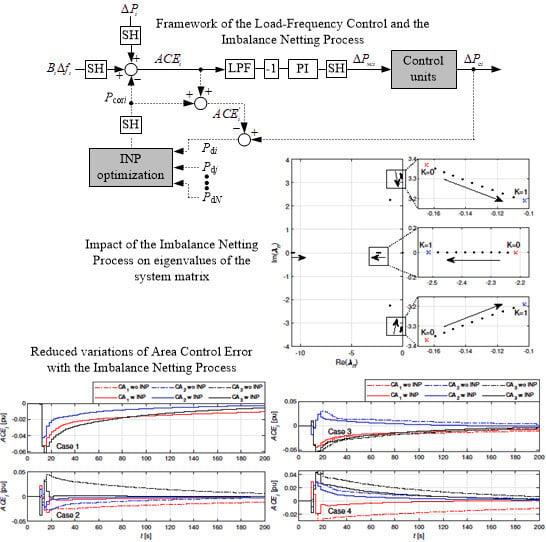
2. Load-Frequency Control and the Imbalance Netting Process

2.1. LFC

A large-scale power system comprises multiple CAs that are connected through transmission lines. In addition to frequency control within each CA, interchange power with neighboring CAs must also be controlled, which is known as LFC [10]. The input of LFC is an area control error, which is, for the i-th CA, defined as

$$AC{E}_i^{\prime }=\Delta P_i+B_i\Delta f_i,$$

(1)

where $\Delta f_i=(f_{\mathrm{a}i}-f_{\mathrm{s}i})$ and $\Delta P_i=(P_{\mathrm{a}i}-P_{\mathrm{s}i})$ are frequency deviation and interchange power variation, respectively. Here, $f_{\mathrm{a}i}$ and $P_{\mathrm{a}i}$ denote actual, i.e., measured, values, while $f_{\mathrm{s}i}$ and $P_{\mathrm{s}i}$ denote scheduled values. Furthermore, $B_i$ is the frequency-bias coefficient that reflects the size of the CA. The value of $B_i$ is determined on an annual basis by all TSOs of a synchronous area, considering the sum of primary control reserve relative to the maximum steady-state frequency deviation, the auto-control of generation, and the self-regulation of load [11]. Note that $AC{E}_i^{\prime }<0$ means that the consumption is higher than the generation; therefore, the CA is characterized as “short”. Furthermore, a CA is characterized as “long” when $AC{E}_i^{\prime }>0$.

The basic LFC framework of the i-th CA is shown in Figure 1 with solid lines. Here, PI is a proportional-integral controller, whereas a negative control-feedback is included as −1 gain. In addition, LPF denotes low pass filter and SH denotes sample and hold, with typical values of a sampling time $T_{\mathrm{s}}$ between 1 to 5 s. The output of LFC is scheduled control power $\Delta P_{\mathrm{sc}i}$, which is distributed to the participating control units that change active electric power $\Delta P_{\mathrm{e}i}$ accordingly. When neglecting the transmission losses, the electrical control power of the i-th CA can be expressed as

$$\Delta P_{\mathrm{e}i}=\Delta P_i+\Delta P_{\mathrm{L}i},$$

(2)

where $\Delta P_{\mathrm{L}i}$ denotes load power variation. Undoubtedly, the provision of LFC is an expense for the TSO, which depends on the size of the LFC reserve, and on the actually activated reserve power. Note, the LFC reserve is also known as a regulating reserve, whereas, instead of activated reserve power, the term balancing energy is used, typically.

2.2. INP

INP was developed due to the high costs of balancing energy, where CAs with opposite signs of interchange power variations can net the demand for balancing energy between the participating CAs [7,20]. Compensation between CAs is possible if participating CAs have different signs of demand power; thus, CAs with a surplus of energy, i.e., “long” CAs, can compensate CAs with a shortage of energy, i.e., “short” CAs. Thus, the balancing energy can be decreased, while releasing regulating reserve. Participating CAs are connected by an INP optimization module through virtual tie-lines. Note that a virtual tie-line connects control units in the CA of the connecting TSO to the CA of the receiving TSO. The active power flow on a virtual tie-line is either measured or calculated from the measurements [11].

The framework of an LFC with INP optimization module is shown in Figure 1 with solid and dotted lines. The input variables for INP optimization are the demand powers of all participating CAs; i.e., $P_{\mathrm{d}i}$, $P_{\mathrm{d}j}$,…, $P_{\mathrm{d}N}$. The demand power of the i-th CA determines the total compensation power with participating CAs that have the opposite sign of $AC{E}_i^{\prime }$, and is given as

$$P_{\mathrm{d}i}=\Delta P_{\mathrm{e}i}-AC{E}_i^{\prime }.$$

(3)

The following relation is obtained by introducing (1) and (2) into (3)

$$P_{\mathrm{d}i}=\Delta P_{\mathrm{L}i}-B_i\Delta f_i.$$

(4)

The output variable of the INP optimization is a correction power $P_{\mathrm{cor}i}$, calculated with a delay of $T_{\mathrm{s}}$ due to SH. It is included for the i-th CA as

$$AC{E}_i=(\Delta P_i+B_i\Delta f_i)-P_{\mathrm{cor}i},$$

(5)

where terms in brackets denote $AC{E}_i^{\prime }$. Clearly, $P_{\mathrm{cor}i}$ and $P_{\mathrm{d}i}$ must have opposite signs. Note that compensation between the i-th and j-th CA is possible only if $\mathrm{sign}\left(P_{\mathrm{d}i}\right)\ne \mathrm{sign}\left(P_{\mathrm{d}j}\right)$.

Calculation of $P_{\mathrm{cor}i}$ is a part of the INP optimization that is explained in the next Section. However, in the case of two participating CAs, only two corrections are possible; i.e., $P_{\mathrm{cor}i}=-P_{\mathrm{d}i}K$ or $P_{\mathrm{cor}i}=+P_{\mathrm{d}j}K$. Here, factor K accounts for the limit of ATC, where $K=0$ means that INP compensation is equal to 0%, whereas $K=1$ means that INP compensation is equal to 100%. When considering (4), the correction between two participating CAs is, for the i-th CA, expressed as

$$P_{\mathrm{cor}i}=(-\Delta P_{\mathrm{L}i}+B_i\Delta f_i)K$$

(6)

or

$$P_{\mathrm{cor}i}=(\Delta P_{\mathrm{L}j}-B_j\Delta f_j)K.$$

(7)

2.3. INP Optimization

The main target function of INP optimization is the maximal possible compensation, with a general limit of $P_{\mathrm{d}i}$ and the limit of ATC between participating CAs, which can differ for each direction of compensation. When connecting various CAs through one common point, a target function of fairness is considered, additionally, which distributes $P_{\mathrm{cor}i}$ between participating CAs. Generally, a proportional to imbalance distribution is used, but inverse ratio to imbalance, or uniform pro-rata distributions could also be used [8]. Moreover, in cases of parallel tie-lines, an additional target function is needed for advantageous use of the tie-lines with the highest ATC. Economic optimization, which minimizes the costs of participating CAs, is also possible. Note, this paper does not discuss INP optimization while proportional to imbalance distribution is used.

3. Eigenvalue Analysis of a Two CA System with INP

A linearized fourth order system with constant parameters is used to describe the i-th CA, as proposed in [10,14]. Generator and load dynamics are represented by inertia $H_i$ and damping $D_i$. A governor-turbine system is described as a steam non-reheat turbine with time constants $T_{\mathrm{G}i}$ and $T_{\mathrm{CH}i}$. A primary frequency loop is considered with a constant droop characteristic $R_i$. Moreover, LFC is modeled by a PI controller with a gain $K_{\mathrm{r}i}$ and time constant $T_{\mathrm{r}i}$. In addition, INP is also included according to Figure 1, where ATC is considered with a factor K, as described in Section 2.2. The physical connection between CA${}_i$–CA${}_j$ is described by a synchronizing coefficient $T_{ij}$ that is defined with parameters of a lossless equivalent tie-line in the vicinity of the operating point. Note that LPF and time delays due to the SH are not considered.

3.1. State-Space Model

Two CAs connected through a tie-line represent a ninth order system, which, in a state-space matrix representation, is given as

$$\dot{\mathbf{x}}=\mathbf{A}\mathbf{x}+\mathbf{B}\mathbf{u}.$$

(8)

Vectors of state-space and input variables are given, respectively, as

$$\begin{array}{lll}{\mathbf{x}}^{\mathrm{T}}& = & [\Delta f_1,\Delta P_{\mathrm{m}1},\Delta P_{\mathrm{g}1},\int AC{E}_{1}dt,\\ & & \Delta f_2,\Delta P_{\mathrm{m}2},\Delta P_{\mathrm{g}2},\int AC{E}_{2}dt,\Delta P_{12}]\hfill \end{array}$$

(9)

and

$${\mathbf{u}}^{\mathrm{T}}=[\Delta P_{\mathrm{L}1},\Delta P_{\mathrm{L}2}],$$

(10)

where $\Delta P_{\mathrm{g}1}$ and $\Delta P_{\mathrm{g}2}$ are the turbine governor’s outputs, and $\Delta P_{\mathrm{m}1}$ and $P_{\mathrm{m}2}$ are turbine outputs. System and input matrices $\mathbf{A}$ and $\mathbf{B}$ both depend on the state of the INP optimization. For two participating CAs, the only possibility for correction power is given as $P_{\mathrm{cor}1}=-P_{\mathrm{cor}2}$, whereas two states of the INP optimization are possible; i.e.,

State 1: 

$P_{\mathrm{cor}1}=-P_{\mathrm{d}1}K$, $P_{\mathrm{cor}2}=+P_{\mathrm{d}1}K$;

State 2: 

$P_{\mathrm{cor}1}=+P_{\mathrm{d}2}K$, $P_{\mathrm{cor}2}=-P_{\mathrm{d}2}K$.

It should be emphasized that INP switches between both states. However, the constant structure of the model is further assumed; thus, both states will be analyzed separately. Due to INP, ATC factor K appears in matrices $\mathbf{A}$ and $\mathbf{B}$; thus, $K=0$ corresponds to a system without INP. When considering the INP given in Section 2.2, then matrices $\mathbf{A}$ and $\mathbf{B}$ are given by (11) for State 1, and by (12) for State 2.

$$\mathbf{A}=\left[\begin{array}{ccccccccc}-\frac{D_1}{2H_1}& \frac{1}{2H_1}& 0& 0& 0& 0& 0& 0& -\frac{1}{2H_1}\\ 0& -\frac{1}{T_{\mathrm{CH}1}}& \frac{1}{T_{\mathrm{CH}1}}& 0& 0& 0& 0& 0& 0\\ -\frac{1+R_1{K}_{\mathrm{r}1}{B}_1(1-K)}{R_1{T}_{\mathrm{G}1}}& 0& -\frac{1}{T_{\mathrm{G}1}}& -\frac{K_{\mathrm{r}1}}{T_{\mathrm{G}1}{T}_{\mathrm{r}1}}& 0& 0& 0& 0& -\frac{K_{\mathrm{r}1}}{T_{\mathrm{G}1}}\\ B_1(1-K)& 0& 0& 0& 0& 0& 0& 0& 1\\ 0& 0& 0& 0& -\frac{D_2}{2H_2}& \frac{1}{2H_2}& 0& 0& \frac{1}{2H_2}\\ 0& 0& 0& 0& 0& -\frac{1}{T_{\mathrm{CH}2}}& \frac{1}{T_{\mathrm{CH}2}}& 0& 0\\ -\frac{K_{\mathrm{r}2}{B}_{1}K}{T_{\mathrm{G}2}}& 0& 0& 0& -\frac{1+R_2{K}_{\mathrm{r}2}{B}_2}{R_2{T}_{\mathrm{G}2}}& 0& -\frac{1}{T_{\mathrm{G}2}}& -\frac{K_{\mathrm{r}2}}{T_{\mathrm{G}2}{T}_{\mathrm{r}2}}& \frac{K_{\mathrm{r}2}}{T_{\mathrm{G}2}}\\ B_{1}K& 0& 0& 0& B_2& 0& 0& 0& -1\\ 2\pi T_{12}& 0& 0& 0& -2\pi T_{12}& 0& 0& 0& 0\end{array}\right],\mathbf{B}=\left[\begin{array}{cc}-\frac{1}{2H_1}& 0\\ 0& 0\\ -\frac{K_{\mathrm{r}1}K}{T_{\mathrm{G}1}}& 0\\ K& 0\\ 0& -\frac{1}{2H_2}\\ 0& 0\\ \frac{K_{\mathrm{r}2}K}{T_{\mathrm{G}2}}& 0\\ -K& 0\\ 0& 0\end{array}\right].$$

(11)

$$\mathbf{A}=\left[\begin{array}{ccccccccc}-\frac{D_1}{2H_1}& \frac{1}{2H_1}& 0& 0& 0& 0& 0& 0& -\frac{1}{2H_1}\\ 0& -\frac{1}{T_{\mathrm{CH}1}}& \frac{1}{T_{\mathrm{CH}1}}& 0& 0& 0& 0& 0& 0\\ -\frac{1+R_1{K}_{\mathrm{r}1}{B}_1}{R_1{T}_{\mathrm{G}1}}& 0& -\frac{1}{T_{\mathrm{G}1}}& -\frac{K_{\mathrm{r}1}}{T_{\mathrm{G}1}{T}_{\mathrm{r}1}}& -\frac{K_{\mathrm{r}1}{B}_{2}K}{T_{\mathrm{G}1}}& 0& 0& 0& -\frac{K_{\mathrm{r}1}}{T_{\mathrm{G}1}}\\ B_1& 0& 0& 0& B_{2}K& 0& 0& 0& 1\\ 0& 0& 0& 0& -\frac{D_2}{2H_2}& \frac{1}{2H_2}& 0& 0& \frac{1}{2H_2}\\ 0& 0& 0& 0& 0& -\frac{1}{T_{\mathrm{CH}2}}& \frac{1}{T_{\mathrm{CH}2}}& 0& 0\\ 0& 0& 0& 0& -\frac{1+R_2{K}_{\mathrm{r}2}{B}_2(1-K)}{R_2{T}_{\mathrm{G}2}}& 0& -\frac{1}{T_{\mathrm{G}2}}& -\frac{K_{\mathrm{r}2}}{T_{\mathrm{G}2}{T}_{\mathrm{r}2}}& \frac{K_{\mathrm{r}2}}{T_{\mathrm{G}2}}\\ 0& 0& 0& 0& B_2(1-K)& 0& 0& 0& -1\\ 2\pi T_{12}& 0& 0& 0& -2\pi T_{12}& 0& 0& 0& 0\end{array}\right],\mathbf{B}=\left[\begin{array}{cc}-\frac{1}{2H_1}& 0\\ 0& 0\\ 0& \frac{K_{\mathrm{r}1}K}{T_{\mathrm{G}1}}\\ 0& -K\\ 0& -\frac{1}{2H_2}\\ 0& 0\\ 0& -\frac{K_{\mathrm{r}2}K}{T_{\mathrm{G}2}}\\ 0& K\\ 0& 0\end{array}\right].$$

(12)

3.2. Numerical Evaluation of the Impact of the ATC Factor on the Eigenvalues of $\mathbf{A}$

A numerical evaluation was performed, since exact analytical expressions for eigenvalues are complicated. Two identical CAs were assumed, with typical parameters and control settings [10,14]. The only differences were PI controller time constants, which were $T_{\mathrm{r}1}=$ 60 s and $T_{\mathrm{r}2}=$ 30 s. ATC factor K was considered as a free parameter. Only INP was considered, since it affects the matrix $\mathbf{A}$. The obtained characteristic polynomial is given as

$$\sum _{n=0}^9{a}_n{\lambda }^n,$$

(13)

where $\lambda$ is an eigenvalue of $\mathbf{A}$, whereas coefficients $a_n$ are given in

Table 1. Coefficients of a characteristic polynomial.

State 1	$a_0$	$a_1$	$a_2$	$a_3$	$a_4$	$a_5$	$a_6$	$a_7$	$a_8$	$a_9$
	0.6	30K + 233	−19K + 20,000	−1300K + 21,000	−599K + 12,000	−233K + 4800	−17K + 1200	255	27	1
State 2	$a_0$	$a_1$	$a_2$	$a_3$	$a_4$	$a_5$	$a_6$	$a_7$	$a_8$	$a_9$
	0.6	−30K + 233	−59K + 20,000	−1300K + 21,000	−599K + 12,000	−233K + 4800	−17K + 1200	255	27	1

for both the discussed States.

Figure 2 shows the impact of the ATC factor K on eigenvalues of $\mathbf{A}$ for INP and State 1. A dominant impact of factor K is noticed on three eigenvalues, where one is real and two are complex conjugates, as shown in Figure 2. They are determined by coefficients $a_2$, $a_5$ and $a_6$. The most critical are complex conjugate eigenvalues, since increasing the ATC factor K results in decrease of the damping $\zeta$, as given in

Table 2. The impacts of ATC factor K on the damping of dominant complex conjugate eigenvalues of $\mathbf{A}$.

State 1	K	0	0.1	0.2	0.3	0.4	0.5	0. 6	0.7	0.8	0.9	1
	$\zeta$	0.0571	0.0558	0.0544	0.0529	0.0514	0.0498	0.0481	0.0463	0.0445	0.0425	0.0405
State 2	K	0	0.1	0.2	0.3	0.4	0.5	0. 6	0.7	0.8	0.9	1
	$\zeta$	0.0571	0.0558	0.0544	0.0530	0.0514	0.0498	0.0481	0.0464	0.0445	0.0426	0.0406

and Figure 3, and has negative impact on the system. The results are given for moderately coupled systems. Additionally, different values of the tie-line parameter $T_{ij}$ were used to show the impact of ATC factor K on damping of dominant eigenvalues of $\mathbf{A}$. Figure 3 shows clearly that an increase of $T_{ij}$ results in a decrease of $\zeta$, in addition to the decrease of $\zeta$ with an increase of K. Note that the results obtained for State 2 are similar and the differences are seen in Table 1 and Table 2.

4. Numerical Simulations and Performance Indicators

A testing system with three equal CAs was considered, where CA${}_1$–CA${}_2$ and CA${}_2$–CA${}_3$ were connected with tie-lines, whereas CA${}_1$–CA${}_3$ were not connected physically through a tie-line. Moreover, all three CAs were connected by the INP optimization module through virtual tie-lines. A Matlab/SIMULINK model was developed, wherein numerical simulations were performed using a 50 ms step-size.

4.1. Dynamic Model

4.1.1. Structure

A single CA was described with a linearized low-order model [14,24], as shown in Figure 4. The model assumes that voltage control (reactive power) does not affect frequency control (active power). Furthermore, a group of several generators was replaced with one equivalent, where the fast (voltage and angle) dynamic was neglected, which reduced the complexity of the modeling. Therefore, generator–load dynamic is described by $H_i$ and $D_i$. Additionally, three different types of governor-turbine systems were considered; i.e., a hydraulic unit, a steam reheat unit and a steam non-reheat unit, that is presented as

$$M_{1i}={\displaystyle \frac{1}{1+s{T}_{\mathrm{G}i}}}\frac{1+s{T}_{\mathrm{R}i}}{1+(R_{\mathrm{T}i}/R_{\mathrm{P}i})s{T}_{\mathrm{R}i}}\frac{1-s{T}_{\mathrm{W}i}}{1+s0.5T_{\mathrm{W}i}},$$

(14)

$$M_{2i}={\displaystyle \frac{1}{1+s{T}_{\mathrm{G}i}}}\frac{1+s{F}_{\mathrm{HP}i}{T}_{\mathrm{RH}i}}{(1+s{T}_{\mathrm{CH}i})(1+s{T}_{\mathrm{RH}i})},$$

(15)

$$M_{3i}={\displaystyle \frac{1}{1+s{T}_{\mathrm{G}i}}}\frac{1}{1+s{T}_{\mathrm{CH}i}},$$

(16)

respectively [10]. Here, $T_{\mathrm{G}i}$ denotes the governor time constant, $T_{\mathrm{R}i}$ is the reset time, $R_{\mathrm{T}i}$ is the temporary droop, $R_{\mathrm{P}i}$ is the permanent droop and $T_{\mathrm{W}i}$ is the water starting time. Moreover, $F_{\mathrm{HP}i}$ is a fraction of the total turbine power generated by the high pressure turbine section, $T_{\mathrm{CH}i}$ is the time constant of the main inlet volumes and steam chest, whereas $T_{\mathrm{RH}i}$ is the time constant of the reheater. A constant $R_{\mathrm{n}i}$ was assumed, in addition to the ramping rate and participation factors ${\alpha }_{\mathrm{n}i}$ of the control units. Furthermore, a first order LPF and a PI controller were modeled as

$$G_{\mathrm{LPF}i}=\frac{1}{1+s{T}_{\mathrm{LPF}i}},$$

(17)

$$G_{\mathrm{r}i}=K_{\mathrm{r}i}\frac{1+s{T}_{\mathrm{r}i}}{s{T}_{\mathrm{r}i}}.$$

(18)

Here, $T_{\mathrm{LPF}i}$ denotes the LPF time constant, whereas $K_{\mathrm{r}i}$ is gain and $T_{\mathrm{r}i}$ is the time constant of the PI controller. The tie-line connection with various CAs was described by $T_{ij}$, which is defined with line reactance, magnitude and angle difference of the line terminal bus voltage [25]. Furthermore, two different structures were used; i.e., with and without INP.

4.1.2. Parameters

The parameters of the model used for numerical simulations were set according to [10,14] and are given in

Table 3. Model parameters used for numerical simulations.

Parameter	Value	Parameter	Value	Parameter	Value
$H_i$	0.1 pu s	${\alpha }_{\mathrm{n}i}$	1/3	$T_{\mathrm{LPF}i}$	0.3 s
$D_i$	0.01 pu/Hz	$K_{\mathrm{r}i}$	0.3	$T_{\mathrm{r}1}$	60 s
$T_{ij}$	1/15 pu/Hz	$R_{\mathrm{n}i}$	3 Hz/pu	$T_{\mathrm{r}2}=T_{\mathrm{r}3}$	30 s
Hydraulic	Value	Non-Rehat	Value	Reheat	Value
$T_{\mathrm{G}i}$	0.2 s	$T_{\mathrm{G}i}$	0.1 s	$T_{\mathrm{G}i}$	0.2 s
$T_{\mathrm{R}i}$	5 s	$T_{\mathrm{CH}i}$	0.3 s	$T_{\mathrm{RH}i}$	7 s
$T_{\mathrm{W}i}$	1 s	–	–	$T_{\mathrm{CH}i}$	0.3 s
$R_{\mathrm{T}i}/R_{\mathrm{P}i}$	7.6	–	–	$F_{\mathrm{HP}i}$	0.3
ramp rate	±100	ramp rate	±20	ramp rate	±10

, where the ramp rate is given in puMW/min. The frequency-bias coefficient was determined as constant $B_i=(1/R_i+D_i)$, where $1/R_i=1/R_{1i}+1/R_{2i}+1/R_{3i}$. In all three CAs the model parameters were set equally, the only differences were PI controller time constants $T_{\mathrm{r}i}$, which showed the largest impact on $\Delta f_i$. Note that, in addition to $T_{\mathrm{r}i}$, $K_{\mathrm{r}i}$, $T_{\mathrm{LPF}i}$ and ${\alpha }_{\mathrm{n}i}$ also showed an impact on $\Delta f_i$, but it was negligible in comparison to $T_{\mathrm{r}i}$; therefore, their values were set equally for all three CAs. Moreover, one cycle each of AGC and INP optimization was included with $T_{\mathrm{s}}=$ 2 s, respectively.

4.2. Testing Cases

In order to simulate the worst case, the loads of individual CAs were changed simultaneously, although their proportions were maintained through the entire simulation. Note, proportions were set as $|\Delta P_{\mathrm{L}1}|/|\Delta P_{\mathrm{L}2}|=1.5$, $|\Delta P_{\mathrm{L}2}|/|\Delta P_{\mathrm{L}3}|=0.5$ and $|\Delta P_{\mathrm{L}1}|/|\Delta P_{\mathrm{L}3}|=0.75$. Additionally, the limit of ATC for power interchange between CAs was disabled ($K=1$) to achieve maximum possible compensation with INP. All possible sign combinations of $\Delta P_{\mathrm{L}i}$ for numerical simulations of a three-CA testing system are shown in

Table 4. Possible sign combinations of $\Delta P_{\mathrm{L}i}$ for numerical simulations for three CAs.

$\mathbf{Sign}\left(\mathbf{\Delta }{\mathit{P}}_{\mathbf{L}\mathit{i}}\right)$				Possible INP
	CA${}_1$	CA${}_2$	CA${}_3$	Compensation
Case 1	+	+	+	NO
Case 2	+	+	−	YES
Case 3	+	−	+	YES
Case 4	+	−	−	YES
Case 5	−	+	+	YES
Case 6	−	−	+	YES
Case 7	−	+	−	YES
Case 8	−	−	−	NO

in addition to possible INP compensation. Four testing cases were considered; i.e., Cases 1–4, since Cases 5–8 gave the same results, only the resulting signs were opposite. In Case 1, load magnitudes were set in a way that all three CAs were short. In Case 2 CA${}_1$ and CA${}_2$ were short, while CA${}_3$ was long. In Case 3, CA${}_1$ and CA${}_3$ were short, while CA${}_2$ was long. In Case 4, CA${}_1$ was short, while CA${}_2$ and CA${}_3$ were long. Furthermore, full compensation was possible in Cases 2 and 3, due to a higher absolute value of the sum of loads in long CAs in comparison to the absolute value of the load in the short CA. In addition, two types of tests were performed; i.e., step changes of loads and random load fluctuations.

4.2.1. Step Changes of Loads

The initial load values were equal to zero in all three connected CAs, as shown in Figure 5. Then, simultaneous step changes of the loads were applied at $t=$ 10 s.

4.2.2. Random Load Fluctuations

A dynamic load model was considered as a linear, stochastic, time-invariant, first-order system [26]. It was composed from two components, wherein the first one correlated to trend changes with the quasi-period of 10–30 min. The second component captured common fluctuations with the quasi-period of several minutes. The dynamic model parameters were mean value, standard deviation and autocorrelation, which should be known for both components. The discussed parameters were set according to the measurements of an open-loop ACE in an undisclosed CA for a time period of 24 h. The resulting load was changed every 60 s, and is shown in Figure 6.

4.3. Indicators for Evaluation of LFC Provision

Provision of LFC during random load fluctuations was evaluated with performance indicators, balancing energy, regulating reserve and unintended exchange of energy. Note that 15-min averages of the discussed variables was considered, as defined in [11].

4.3.1. Performance Indicators

Provision of LFC is generally evaluated with indicators defined by control performance standards (CPS) [11,12]. Standard deviation of $AC{E}_i$, denoted as ${\sigma }_{ACEi}$, is used as a common indicator, which is also comparable to the performance criterion defined by the European Network of Transmission System Operators (ENTSO-E) [27]. Additionally, it is similar to CPS2, which is given by the North American Electric Reliability Corporation (NERC) [12]. Furthermore, frequency quality was evaluated with standard deviation of $\Delta f_i$, denoted as ${\sigma }_{\Delta fi}$, which is given in [11,12]. The term frequency quality can also be used as a measure of maintaining a good security of supply level; i.e., maintaining the balance between generation and consumption of electrical energy in the power system [28].

4.3.2. Balancing Energy

As stated in [17], it is the energy used by TSOs to perform balancing and provided by a balancing service provider, which is a market participant with reserve-providing units able to provide balancing services to TSOs. Electricity balancing encompasses all actions and processes, on all timelines, through which TSOs ensure, in a continuous way, the system frequency is within a predefined stability range. By definition, this is the actually activated electrical control power that can be, for the observed time period, calculated as $\Delta W_{\mathrm{e}i}={\int }_0^t\Delta P_{\mathrm{e}i}dt$. Calculation was performed separately for positive and negative values, which is, respectively, denoted as $\Delta W_{\mathrm{e}i+}$ and $\Delta W_{\mathrm{e}i-}$.

4.3.3. Regulating Reserve

According to [29], it is an amount of spinning reserve responsive to AGC, which is sufficient to provide a normal regulating margin. The amount of regulating reserve can be estimated with mean value and standard deviation of $\Delta P_{\mathrm{sc}i}$, denoted as ${\mu }_{\Delta P_{\mathrm{sc}i}}$ and ${\sigma }_{\Delta P_{\mathrm{sc}i}}$. They should be calculated separately for positive and negative values, which are, respectively, denoted as ${\mu }_{\Delta P_{\mathrm{sc}i+}}$, ${\mu }_{\Delta P_{\mathrm{sc}i-}}$ and ${\sigma }_{\Delta P_{\mathrm{sc}i+}}$, ${\sigma }_{\Delta P_{\mathrm{sc}i-}}$.

4.3.4. Unintended Exchange of Energy

By definition, this is the difference between scheduled exchanges and measured physicals flows of electrical energy between TSOs. In addition to interchange power variation, correction power should also be considered [17]. Consequently, unintended exchange of energy for the observed time period, is calculated as $(\Delta W_i-\Delta W_{\mathrm{cor}i})={\int }_0^t(\Delta P_i-\Delta P_{\mathrm{cor}i})dt$. Calculations were preformed separately for positive and negative values, which are, respectively, denoted as $\Delta W_{\mathrm{un}+}$ and $\Delta W_{\mathrm{un}-}$.

5. Results

Numerical simulations were performed for a three-CA testing system in order to analyze the impact of INP on the system’s response. The impact was evaluated according to the results obtained.

5.1. Time Responses to Step Changes of Loads

Results are shown in Figure 7, Figure 8, Figure 9, Figure 10, Figure 11, Figure 12 and Figure 13. Frequency deviations $\Delta f_i$ in all three CAs are seen in Figure 7a–d after step changes of loads were applied. In Cases 1–3, $\Delta f_i$ is negative due to the positive value of total $\Delta P_{\mathrm{L}i}$, which is $\sum \Delta P_{\mathrm{L}i}=+0.09$ for Case 1, $\sum \Delta P_{\mathrm{L}i}=+0.01$ for Case 2 and $\sum \Delta P_{\mathrm{L}i}=+0.05$ for Case 3. However, in Case 4, $\Delta f_i$ is positive due to the negative value of the total $\Delta P_{\mathrm{L}i}$, which is $\sum \Delta P_{\mathrm{L}i}=-0.03$. Note, the first peak of $\Delta f_1$ and $\Delta f_2$ is negative, due to the positive value of $\Delta P_{\mathrm{L}1}$ and $\Delta P_{\mathrm{L}2}$ in Case 2. Accordingly, the first peak of $\Delta f_1$ and $\Delta f_3$ is negative due to the positive value of $\Delta P_{\mathrm{L}1}$ and $\Delta P_{\mathrm{L}3}$ in Case 3, whereas the first peak of $\Delta f_1$ is negative, due to the positive value of $\Delta P_{\mathrm{L}1}$ in Case 4. Initially, primary frequency control decreases $\Delta f_i$ in approximately 30 s after the step change of the loads; then, additionally, LFC decreases $\Delta f_i$ slowly. Moreover, INP impacts $\Delta f_i$ in Cases 2–4, but only after the completion of the primary frequency control, whereas, in Case 1, INP compensation was not possible, as shown in Table 4. It is seen clearly that, in Cases 2 and 3, INP has decreased $\Delta f_i$ in all three CAs in comparison to the system without INP. However, in Case 4, $\Delta f_i$ was increased due to the negative value of the total $\Delta P_{\mathrm{L}i}$, where full compensation was not possible.

The impact of INP is shown more clearly in Figure 8, Figure 9 and Figure 10. Values of $AC{E}_i$, $\Delta P_{\mathrm{sc}i}$ and $\Delta P_{\mathrm{e}i}$ decreased with INP in Cases 2–4. Note that INP had an insignificant impact on the dynamic of primary frequency control, as seen from $\Delta P_{\mathrm{e}i}$, where, approximately 20 s after the step change of the load, the differences between the systems with and without INP occurred. However, INP obviously increased $\Delta P_i$ in Cases 2–4, due to additional tie-line power flow, as seen in Figure 11. Note, in Case 1, INP compensation was not possible.

The signs of $\Delta P_{\mathrm{d}i}$ and $P_{\mathrm{cor}i}$ are opposite in Cases 2–4, as shown in Figure 12 and Figure 13, and a 2 s time delay is seen in $P_{\mathrm{cor}i}$ due to INP, particularly at the beginning of the transients. Due to the oscillations in $\Delta f_i$, the sign change in $\Delta P_{\mathrm{d}i}$ is obvious. Consequently, $P_{\mathrm{cor}i}$ also changes sign, or can even be zero, as seen in Cases 2 and 3. Therefore, these fast changing compensations are not desirable, since they increase variations of $AC{E}_i$ at the beginning of the transients, as shown in Figure 8. Note, in Case 1, INP compensation was not possible.

5.2. Evaluation of LFC Provision to Random Load Fluctuations

Results are given in

Table 5. Performance indicators for LFC.

		${\mathit{\sigma }}_{\mathbf{\Delta }\mathbf{fi}}\left[\mathbf{mHz}\right]$		${\mathit{\sigma }}_{\mathbf{ACEi}}[\mathbf{pu}\times {10}^3]$				${\mathit{\sigma }}_{\mathbf{\Delta }\mathbf{fi}}\left[\mathbf{mHz}\right]$		${\mathit{\sigma }}_{\mathbf{ACEi}}[\mathbf{pu}\times {10}^3]$
Parameter		wo	w	wo	w	Parameter		wo	w	wo	w
Case 1	CA${}_1$	3.95	3.95	5.51	5.51	Case 3	CA${}_1$	2.64	2.45	5.54	4.14
	CA${}_2$	3.84	3.84	2.13	2.13		CA${}_2$	2.29	2.12	2.18	0.55
	CA${}_3$	3.91	3.91	4.29	4.29		CA${}_3$	2.60	2.42	4.30	3.25
Case 2	CA${}_1$	1.01	0.43	5.53	1.18	Case 4	CA${}_1$	0.64	1.04	5.56	0.38
	CA${}_2$	1.24	0.61	2.16	0.45		CA${}_2$	0.65	1.07	2.15	1.10
	CA${}_3$	1.20	0.51	4.31	0.12		CA${}_3$	0.52	0.93	4.30	2.24

Legend: wo—without INP; w—with INP.

,

Table 6. Indicators for regulating reserve and balancing energy.

		CA${}_1$		CA${}_2$		CA${}_3$
Parameter		wo	w	wo	w	wo	w
Case 1	${\mu }_{P\mathrm{sc}i+}[\mathrm{pu}\times {10}^3]$	20.22	20.22	13.49	13.49	27.01	27.01
	${\mu }_{P\mathrm{sc}i™}[\mathrm{pu}\times {10}^3]$	−13.75	−13.75	−9.66	−9.66	−19.36	−19.36
	${\sigma }_{P\mathrm{sc}i+}[\mathrm{pu}\times {10}^3]$	14.03	14.03	9.75	9.75	19.55	19.55
	${\sigma }_{P\mathrm{sc}i-}[\mathrm{pu}\times {10}^3]$	10.88	10.88	7.49	7.49	14.98	14.98
	$\Delta W_{\mathrm{e}i+}\left[\mathrm{pu}\mathrm{h}\right]$	4.43	4.43	3.10	3.10	6.02	6.02
	$\Delta W_{\mathrm{e}i-}\left[\mathrm{pu}\mathrm{h}\right]$	−2.35	−2.35	−1.70	−1.70	−3.23	−3.23
Case 2	${\mu }_{P\mathrm{sc}i+}[\mathrm{pu}\times {10}^3]$	20.24	4.15	13.52	2.84	19.39	0.31
	${\mu }_{P\mathrm{sc}i-}[\mathrm{pu}\times {10}^3]$	−13.77	−2.86	−9.69	−1.98	−27.04	−0.33
	${\sigma }_{P\mathrm{sc}i+}[\mathrm{pu}\times {10}^3]$	14.08	2.86	9.79	1.97	15.03	0.24
	${\sigma }_{P\mathrm{sc}i-}[\mathrm{pu}\times {10}^3]$	10.89	2.25	7.51	1.56	19.63	0.21
	$\Delta W_{\mathrm{e}i+}\left[\mathrm{pu}\mathrm{h}\right]$	4.39	0.91	3.01	0.63	3.14	0.03
	$\Delta W_{\mathrm{e}i-}\left[\mathrm{pu}\mathrm{h}\right]$	−2.33	−0.49	−1.62	−0.35	−5.90	−0.04
Case 3	${\mu }_{P\mathrm{sc}i+}[\mathrm{pu}\times {10}^3]$	20.23	14.83	9.49	1.42	27.03	20.09
	${\mu }_{P\mathrm{sc}i-}[\mathrm{pu}\times {10}^3]$	−13.76	−10.19	−13.80	−1.69	−19.37	−13.95
	${\sigma }_{P\mathrm{sc}i+}[\mathrm{pu}\times {10}^3]$	14.06	10.16	7.61	1.14	19.57	14.03
	${\sigma }_{P\mathrm{sc}i-}[\mathrm{pu}\times {10}^3]$	10.90	7.98	9.76	1.03	15.00	11.06
	$\Delta W_{\mathrm{e}i+}\left[\mathrm{pu}\mathrm{h}\right]$	4.41	3.24	1.58	0.16	6.00	4.39
	$\Delta W_{\mathrm{e}i-}\left[\mathrm{pu}\mathrm{h}\right]$	−2.34	−1.74	−2.95	−1.19	−3.22	−2.39
Case 4	${\mu }_{P\mathrm{sc}i+}[\mathrm{pu}\times {10}^3]$	20.25	0.67	9.69	4.91	19.38	9.67
	${\mu }_{P\mathrm{sc}i-}[\mathrm{pu}\times {10}^3]$	−13.78	−0.60	−13.52	−7.07	−27.03	−13.96
	${\sigma }_{P\mathrm{sc}i+}[\mathrm{pu}\times {10}^3]$	14.10	0.42	7.51	3.87	15.01	7.68
	${\sigma }_{P\mathrm{sc}i-}[\mathrm{pu}\times {10}^3]$	10.91	0.43	9.79	4.89	19.61	9.75
	$\Delta W_{\mathrm{e}i+}\left[\mathrm{pu}\mathrm{h}\right]$	4.40	0.11	1.57	0.84	3.15	1.64
	$\Delta W_{\mathrm{e}i-}\left[\mathrm{pu}\mathrm{h}\right]$	−2.34	−0.10	−2.95	−1.55	−5.92	−3.03

Legend: wo—without INP; w—with INP.

and

Table 7. Indicators for unintended exchange of energy.

		$\mathbf{\Delta }{\mathit{W}}_{\mathbf{un}}+\left[\mathbf{pu}\mathbf{h}\right]$		$\mathbf{\Delta }{\mathit{W}}_{\mathbf{un}}-\left[\mathbf{pu}\mathbf{h}\right]$				$\mathbf{\Delta }{\mathit{W}}_{\mathbf{un}}+\left[\mathbf{pu}\mathbf{h}\right]$		$\mathbf{\Delta }{\mathit{W}}_{\mathbf{un}}-\left[\mathbf{pu}\mathbf{h}\right]$
Parameter		wo	w	wo	w	Parameter		wo	w	wo	w
Case 1	CA${}_1$	0.246	0.246	−0.258	−0.258	Case 3	CA${}_1$	4.444	0.021	−2.368	−0.017
	CA${}_2$	0.273	0.273	−0.263	−0.263		CA${}_2$	0.774	−0.002	−1.460	0.002
	CA${}_3$	0.086	0.086	−0.075	−0.075		CA${}_3$	1.597	0.022	−2.986	−0.026
Case 2	CA${}_1$	1.935	0.019	−3.604	−0.023	Case 4	CA${}_1$	2.368	0.017	−4.444	−0.021
	CA${}_2$	1.269	−0.008	−2.378	0.009		CA${}_2$	1.460	−0.002	−0.774	0.002
	CA${}_3$	5.982	0.013	−3.204	−0.011		CA${}_3$	2.986	0.026	−1.597	−0.022

Legend: wo—without INP; w—with INP.

and Figure 14. Performance indicators ${\sigma }_{\Delta fi}$ and ${\sigma }_{ACEi}$ are given in Table 5. Clearly, INP decreases ${\sigma }_{\Delta fi}$ in Cases 2 and 3, whereas, in Case 4, ${\sigma }_{\Delta fi}$ is increased due to the negative value of the total $\Delta P_{\mathrm{L}i}$, where full compensation was not possible. Moreover, INP decreases ${\sigma }_{ACEi}$ in Cases 1–3, which is obviously expected. In addition, ${\sigma }_{\Delta fi}$ for different values of $T_{ij}$ is shown in Figure 14. Clearly, INP decreases ${\sigma }_{\Delta fi}$ in Cases 2 and 3, whereas, in Case 4, ${\sigma }_{\Delta fi}$ is increased, as expected according to Table 5. However, the impact of $T_{ij}$ on ${\sigma }_{\Delta fi}$ is not unambiguous, since cases of improvement and deterioration exist with the variations of $T_{ij}$. Note, in Case 1, INP compensation was not possible.

Moreover, Table 6 shows the results for the regulating reserve and balancing energy, where INP decreased ${\mu }_{P\mathrm{sc}i}$, ${\sigma }_{P\mathrm{sc}i}$ and $\Delta W_{\mathrm{e}i}$ for positive and negative values in Cases 2–4. This indicates clearly that INP releases regulating reserve and reduces balancing energy. Note, in Case 1, INP compensation was not possible.

Last but not least, results for unintended exchange of energy are given in Table 7. Positive and negative values of $\Delta W_{\mathrm{un}}$ were decreased due to INP in Cases 2–4. Note, in Case 1, INP compensation was not possible.

6. Conclusions

The impact of INP on power system dynamics was shown in this paper. Eigenvalue analysis of a two CA testing system showed clearly, that INP impacts both the system and input matrices. Moreover, from the results obtained it was concluded that INP results in decreased damping of dominant eigenvalues, which has a negative impact on the entire power system’s dynamics. Furthermore, it was shown that increasing the tie-line parameter results in decrease of the damping of the system. In addition, thorough numerical simulations of a three-CA testing system with INP were performend, in order to analyze the impact of INP on frequency quality and provision of LFC. First, from the results of step changes of loads it can be concluded that INP impacts the frequency response of participating CAs. Clearly, INP had a positive impact on frequency quality in cases of positive values of total load variation, whereas a negative value of total load variation had a negative impact of INP frequency quality. In addition, the impact of INP on the dynamic of primary frequency control was negligible. Furthermore, ACE variations were reduced with INP. Moreover, scheduled control and active electric power were reduced, whereas interchange power variation was increased due to higher tie-line power flow between interconnected CAs. A 2 s time delay exists in correction power due to INP, and a sign change in demand power occurred because of the oscillations in frequency deviations. Consequently, correction power changed sign or was zero. Therefore, these fast changing compensations are not desirable, since they increase variations of ACE at the beginnings of the transients.

The results of random load fluctuations confirmed that INP impacts the frequency responses of participating CAs. However, similar to step changes of loads, cases of frequency quality improvement and deterioration exist. Similarly, the impact of tie-line parameter on the standard deviation of frequency deviation is not unambiguous, since cases of improvement and deterioration exist.

A positive value of total load variation had a positive impact of INP on standard deviation of frequency deviation, whereas a negative value of total load variation had negative impact of INP on standard deviation of frequency deviation. Similarly, the standard deviation of ACE was reduced with INP. Moreover, the mean value and standard deviation of scheduled control power for positive and negative values were reduced with INP. Positive and negative balancing energy were also reduced. Last but not least, positive and negative unintended exchange of energy were reduced significantly due to INP. Therefore, it can be concluded from the results obtained that INP reduces activation of secondary control reserve, and consequently, it reduces balancing energy and releases regulating reserve.

Future work should focus on dynamic dimensioning of regulating reserves with respect to INP. It was shown that INP reduced the overall use of regulating reserves, which has not been taken into consideration for reserve dimensioning. That way, the possible over-dimensioning of a regulating reserve could be decreased.

References

1. Zhou, Q.; Bialek, J.W. Approximate model of European interconnected system as a benchmark system to study effects of cross-border trades. IEEE Trans. Power Syst. 2005, 20, 782–788. [Google Scholar] [CrossRef]
2. Ahmadi-Khatir, A.; Conejo, A.J.; Cherkaoui, R. Multi-Area Energy and Reserve Dispatch Under Wind Uncertainty and Equipment Failures. IEEE Trans. Power Syst. 2013, 28, 4373–4383. [Google Scholar] [CrossRef]
3. Bialek, J.W.; Ziemianek, S.; Wallace, R. A methodology for allocating transmission losses due to cross-border trades. IEEE Trans. Power Syst. 2004, 19, 1255–1262. [Google Scholar] [CrossRef]
4. Strasser, T.; Andrén, F.; Kathan, J.; Cecati, C.; Buccella, C.; Siano, P.; Leitão, P.; Zhabelova, G.; Vyatkin, V.; Vrba, P.; et al. A Review of Architectures and Concepts for Intelligence in Future Electric Energy Systems. IEEE Trans. Ind. Electron. 2015, 62, 2424–2438. [Google Scholar] [CrossRef] [Green Version]
5. Blaabjerg, F.; Teodorescu, R.; Liserre, M.; Timbus, A.V. Overview of Control and Grid Synchronization for Distributed Power Generation Systems. IEEE Trans. Ind. Electron. 2006, 53, 1398–1409. [Google Scholar] [CrossRef] [Green Version]
6. Olivares, D.E.; Mehrizi-Sani, A.; Etemadi, A.H.; Cañizares, C.A.; Iravani, R.; Kazerani, M.; Hajimiragha, A.H.; Gomis-Bellmunt, O.; Saeedifard, M.; Palma-Behnke, R.; et al. Trends in Microgrid Control. IEEE Trans. Smart Grid 2014, 5, 1905–1919. [Google Scholar] [CrossRef]
7. Zolotarev, P.; Gökeler, M.; Kuring, M.; Neumann, H.; Kurscheid, E.-M. Grid Control Cooperation—A framework for technical and economical crossborder optimization for load-frequency control. In Proceedings of the 44th International Conference on Large High Voltage Electric Systems (Cigre’12), Paris, France, 26–30 August 2012. [Google Scholar]
8. Scherer, M.; Andersson, G. A blueprint for the European imbalance netting process using multi-objective optimization. In Proceedings of the IEEE International Energy Conference (ENERGYCON’16), Leuven, Belgium, 4–8 April 2016. [Google Scholar]
9. ENTSO-E. Operational Reserve Ad Hoc Team Report; ENTSO-E: Brussels, Belgium, May 2012. [Google Scholar]
10. Kundur, P. Power System Stability and Control; McGraw-Hill: New York, NY, USA, 1994. [Google Scholar]
11. EUR-Lex. Establishing a Guideline on Electricity Transmission System Operation. Commission Regulation (EU) 2017/1485. Available online: https://eur-lex.europa.eu/eli/reg/2017/1485/oj (accessed on 21 October 2019).
12. NERC. Frequency Response Standard, Background Document; NERC: Atlanta, GA, USA, November 2012. [Google Scholar]
13. Jaleeli, N.; VanSlyck, L.S. NERC’s new control performance standards. IEEE Trans. Power Syst. 1999, 14, 1092–1099. [Google Scholar] [CrossRef]
14. Bevrani, H. Robust Power System Frequency Control; Springer: New York, NY, USA, 2009. [Google Scholar]
15. Ilic, M.D.; Yoon, Y.T.; Zobian, A. Available transmission capacity (ATC) and its value under open access. IEEE Trans. Power Syst. 1997, 12, 636–645. [Google Scholar] [CrossRef]
16. Stakeholder Document for the Principles of IGCC; ENTSO-E: Brussels, Belgium, September 2016.
17. EUR-Lex. Establishing a Guideline on Electricity Balancing. Commission Regulation (EU) 2017/2195. Available online: https://eur-lex.europa.eu/eli/reg/2017/2195/oj (accessed on 21 October 2019).
18. Cronenberg, A.; Sager, N.; Willemsen, S. Integration of France into the international grid control cooperation. In Proceedings of the IEEE International Energy Conference (ENERGYCON’16), Leuven, Belgium, 4–8 April 2016. [Google Scholar]
19. Sprey, J.D.; Schultheis, P.; Moser, A. Dynamic dimensioning of balancing reserve. In Proceedings of the 14th International Conference on the European Energy Market (EEM), Dresden, Germany, 6–9 June 2017. [Google Scholar]
20. Supporting Document for the Network Code on Load-Frequency Control and Reserves; ENTSO-E: Brussels, Belgium, June 2013.
21. Oneal, A.R. A simple method for improving control area performance: Area control error (ACE) diversity interchange ADI. IEEE Trans. Power Syst. 1995, 10, 1071–1076. [Google Scholar] [CrossRef]
22. Zhou, N.; Etingov, P.V.; Makarov, J.V.; Guttromson, R.T.; McManus, B. Improving area control error diversity interchange (ADI) program by incorporating congestion constraints. In Proceedings of the IEEE PES T&D 2010, New Orleans, LA, USA, 19–22 April 2010. [Google Scholar]
23. Apostolopoulou, D.; Sauer, P.W.; Dominguez-Garcia, A.D. Balancing authority area coordination with limited exchange of information. In Proceedings of the 2015 IEEE Power and Energy Society General Meeting, Denver, CO, USA, 26–30 July 2015. [Google Scholar]
24. Anderson, P.M.; Mirheydar, M. A low-order system frequency response model. IEEE Trans. Power Syst. 1990, 5, 720–729. [Google Scholar] [CrossRef] [Green Version]
25. Elgerd, O.I.; Fosha, C.E. Optimum megawatt-frequency control of multiarea electric energy systems. IEEE Trans. Power App. Syst. 1970, PAS-89, 556–563. [Google Scholar] [CrossRef]
26. Janecek, E.; Cerny, V.; Fialova, A.; Fantík, J. A new approach to modelling of electricity transmission system operation. In Proceedings of the 2006 IEEE PES Power Systems Conference and Exposition, Atlanta, GA, USA, 29 October–1 November 2006. [Google Scholar]
27. ENTSO-E. Network Code on Load-Frequency Control and Reserves; ENTSO-E: Brussels, Belgium, June 2013. [Google Scholar]
28. ENTSO-E. Frequency Quality, Phase 2; June 2017. [Google Scholar]
29. NERC. Balancing and Frequency Control; NERC: Atlanta, GA, USA, January 2011. [Google Scholar]
Figure 1. Block diagram of the load-frequency control (LFC) framework of the i-th control area (CA) (solid line) with the imbalance netting process (INP) optimization module (solid and dotted line).
Energies 12 04733 g001
Figure 2. Impact of ATC factor K on eigenvalues of A for INP and State 1.
Energies 12 04733 g002
Figure 3. The impacts of available transmission capacity (ATC) factor K on damping of dominant complex conjugate eigenvalues of A for different values of T i j and State 1.
Energies 12 04733 g003
Figure 4. Block diagram of the i-th CA without INP.
Energies 12 04733 g004
Figure 5. Step changes of Δ P L i used in numerical simulations for three CAs.
Energies 12 04733 g005
Figure 6. Random fluctuations of Δ P L i used in numerical simulations for three CAs.
Energies 12 04733 g006
Figure 7. Time response of Δ f i for a three-CA testing system, where “wo” is without INP and “w” is with INP.
Energies 12 04733 g007
Figure 8. Time response of A C E i for a three-CA testing system, where “wo” is without INP and “w” is with INP.
Energies 12 04733 g008
Figure 9. Time response of Δ P sc i for a three-CA testing system, where “wo” is without INP and “w” is with INP.
Energies 12 04733 g009
Figure 10. Time response of Δ P e i for a three-CA testing system, where “wo” is without INP and “w” is with INP.
Energies 12 04733 g010
Figure 11. Time response of Δ P i for a three-CA testing system, where “wo” is without INP and “w” is with INP.
Energies 12 04733 g011
Figure 12. Time response of P d i for a three-CA testing system.
Energies 12 04733 g012
Figure 13. Time response of P cor i for a three-CA testing system.
Energies 12 04733 g013
Figure 14. Calculated σ Δ f i for different values of T i j for a three-CA testing system, where “wo” is without INP and “w” is with INP.
Energies 12 04733 g014