Abstract
This paper develops step-by-step a complete electric model of a light hybrid electric vehicle propulsion system. This model includes the vehicle mass, the radius and mass of the wheels, the aerodynamic profile of the vehicle, the electric motor and the motor drive, among other elements. Each element of the model is represented by a set of equations, which lead to getting an equivalent electric circuit. Based on this model, the outer and inner loop compensators of the motor drive control circuit are designed to provide stability and a fast dynamic response to the system. To achieve this, the steady-state equations and the small-signal model of the equivalent electric circuit are also obtained. Furthermore, as these elements are the main load of the power distribution system of the fully electric and light hybrid electric vehicle, the input impedance model of the set composed of the input filter, the motor drive, the motor, and the vehicle is presented. This input impedance is especially useful to get the system stability of the entire power distribution system.
1. Introduction
The presence of electric vehicles (EV) in the automotive industry is growing rapidly [1]. According to the International Energy Agency, 125 million electric vehicles are expected to be manufactured by 2030 [2]. This growing market requires the optimization of the vehicle design and, therefore, an optimized propulsion system. If the system is too small, the driving range decreases; however, if the system is too big, the cost of the vehicle increases. Thus, the correct sizing is needed to properly design the vehicle.
Power sources such as fuel cells, batteries, and supercapacitors have to manage a power that depends on the power consumption of the vehicle. This power consumption is related to two key factors: the shape and weight of the vehicle and the driving profile.
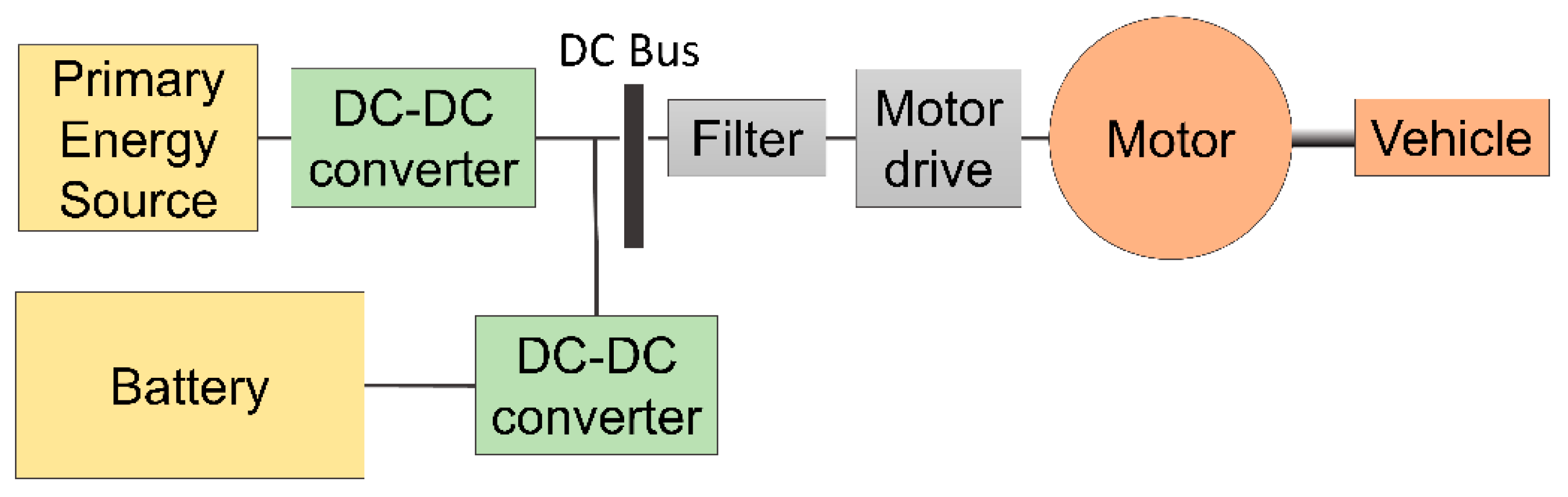
Figure 1 shows, as an example, the block diagram of a hybrid vehicle power distribution system and the main load, composed of the electric motor, the vehicle, the motor drive, and the filter. The vehicle is powered by an electric motor, which needs a motor drive to control its speed and a filter to diminish the propagation of current ripple effects towards the system. The primary energy source, e.g., a fuel cell, needs a DC-DC power converter that adapts and controls its power. The secondary energy source, e.g., a battery, can be connected either directly to the DC bus or via a DC-DC power converter.
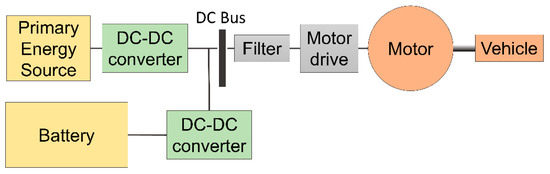
Figure 1.
Block diagram of a hybrid electric vehicle power distribution system.
The vehicle block diagram in Figure 1 shows the different elements in charge of transforming the power sources energy into force and linear speed in the vehicle. This transformation depends on many factors, such as the mass of the vehicle, the radius and the mass of the wheels, and the aerodynamic profile of the vehicle, among others. Besides, the terrain conditions have a considerable influence, e.g., the slope of the terrain and the friction between wheels and road. Another factor could be the environmental conditions such as wind or wet terrain.
Different approaches can be used to model the vehicle. Reviewing the literature, some authors make use of several specific software. ADVISOR® (2002, Nat. Renewable Energy Lab, Golden, CO, USA) is used in [3] to model the vehicle with the aim of developing a power management strategy for an urban driving profile. MATLAB® (2017a, MathWorks, Natick, MA, USA) toolbox PSAT (2.1.11, University College Dublin, Dublin, Ireland) is used in [4] to model Zero-Emission Buses, and SIMULINK® (2019, MathWorks, Natick, MA, USA) is used in [5] to simulate a parallel hybrid powertrain and analyze the fuel consumption.
Another approach is to analyze the forces affecting the vehicle [6,7,8,9,10,11,12,13,14,15]. This approach is used in [6] to develop a sizing method for Hybrid Electric Vehicles (HEV), in [7] to analyze the sensitivity of the performance of a Battery Electric Vehicle (BEV), and in [8,9] to develop the energy consumption model of a plug-in HEV. In addition, this modeling approach is used in [10] to develop a technical assessment of utilizing an electrical variable transmission system in HEV, in [11] this approach is used to model and simulate an electric propulsion system of an EV, and in [12] is used to validate a HEV dynamic model for energy management including tire pressure distribution. Finally, in [13], this modeling approach is used to analyze the drivability of plug-in HEV, including the gear transmissions effects and, in [14,15] is used to design a control strategy for HEV with continuously variable transmission. These models are known as backward-facing vehicle models, which assume that the required demand is always met.
The electric motor model is another key element. State of the art shows that some studies use DC motors [16,17] while other studies use AC motors, e.g., induction motors in [18,19,20], permanent magnet synchronous motors in [18,21,22,23] and, finally, switched reluctance motors in [17,23,24]. The procedure used in each type of motor is similar, although the set of equations and control techniques could be different between them.
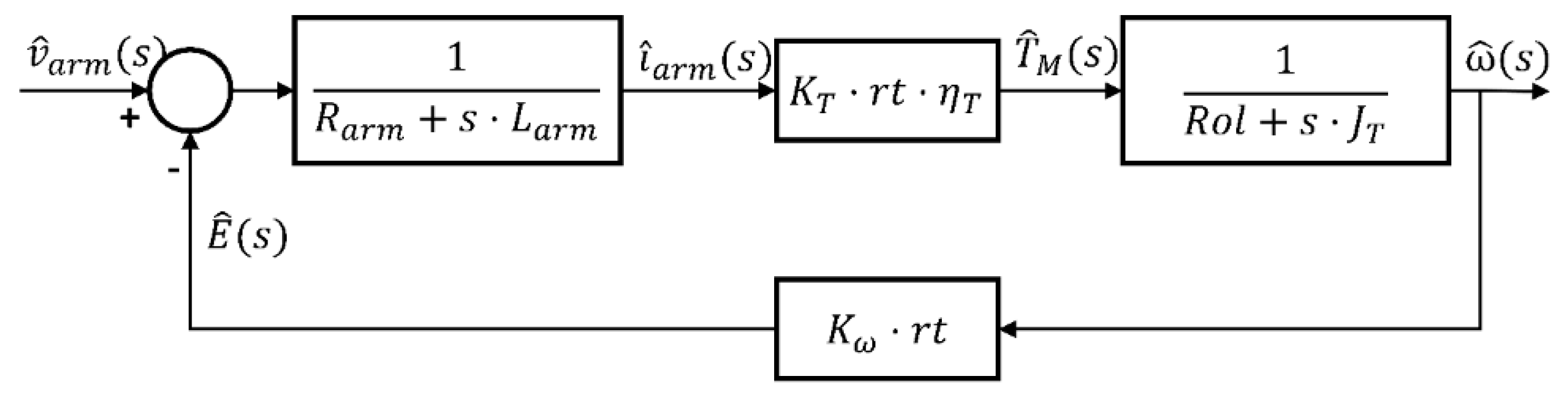
In addition, the electric motor needs a motor drive to control the desired vehicle speed. This motor drive must provide to the entire system good stability and dynamic response, which is achieved with the outer speed loop compensator and the inner current loop compensator, as shown in Figure 2.
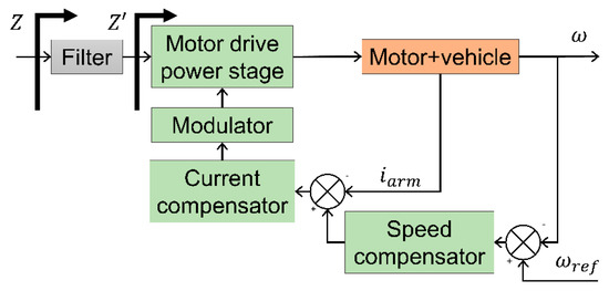
Figure 2.
Block diagram of the motor drive along with the motor and vehicle.
On the other hand, the dynamic of each power converter included in the power distribution system is affected by the other power converters. Thus, the input impedance of the filter-motor drive-electric motor-vehicle combination must be considered to ensure system stability. As shown in Figure 1, the primary energy source, e.g., a fuel cell, is connected to the DC bus via a DC-DC power converter. The secondary energy source, the battery, is also connected to the DC bus via a bidirectional DC-DC power converter. In this type of architecture, stability cannot be guaranteed by default, unlike those architectures with the battery connected directly to the bus. For this reason, the impedance of the loads connected to the DC bus, in this case, the vehicle, motor, motor-drive, and filter, including the speed and current compensator, must be calculated, as shown in Figure 2.
Therefore, one of the main goals of the paper is to develop step-by-step a complete electric model of a light hybrid electric vehicle propulsion system, considering the motor, motor drive, and the light vehicle (including the vehicle mass, the radius and the mass of the wheels, the aerodynamic profile of the vehicle, among others). The model parameter values affect the relationship between the power demanded to the sources and the vehicle speed.
The second goal is to obtain the analytical expression of the small-signal model of the entire system composed of the electric motor, the motor drive (with two control loops), and the vehicle. This analytical expression shows the relationship among the wheel speed, the wheel torque, the electric motor torque, the electric motor current, and the current demanded to the DC bus, in closed-loop.
This model allows developing the electrical simulation and the optimal design of the vehicle power distribution system, as well as to get a controlled speed of the vehicle and a stable system.
Although the modeling procedure can be extended to other types of vehicles, this paper focuses on light vehicles, those whose weight is less than 1000 kg and which are mainly used in cites or in industrial speed-limited areas.
The third main goal is to obtain the input impedance model of the set composed of the input filter, the motor drive, the motor, and the vehicle, which is needed to assure the stability of the entire system. This analytical model results are compared to those obtained from the switched circuit and the averaged circuit simulated with PSIM® (2015, Powersim, Rockville, MD, USA).
As this paper is focused on the motor and the vehicle modeling along with their integration in the entire system, the modeling of other parts of the overall system, e.g., the thermal management, battery management system, fuel cell, etc., are not considered.
The paper is organized as follows. First, Section 2 describes the vehicle and the electric motor model. With this information, the control loop to manage the speed vehicle is developed in Section 3. Next, the electrical input impedance analysis is shown in Section 4. Finally, Section 5 summarizes the main obtained conclusions.
2. Time Domain Modeling of the Vehicle and the Electric Motor
This section presents both the vehicle model and the motor model that allow the power profile to be calculated from a specific driving profile. The vehicle model is presented first, then the motor model is analyzed, and finally, the electric equivalent of both the electric motor and the vehicle is presented.
The vehicle model is based on the analysis of the applied forces on the vehicle and its impact on the electric motor operating conditions. These forces produce a torque on the shaft of the wheel that becomes a torque in the motor shaft.
In order to move the vehicle, the motor has to overcome a resistance torque, TR(t) (N·m), which is composed of two main parts, the torque needed to move the vehicle (acceleration torque) TAccel(t), and the torque to overcome the friction and the aerodynamic drag forces (rolling torque) TRoll(t) (1).
The acceleration torque is composed of the torque needed to move the wheels Twm(t) and the torque needed to move the vehicle Tvm(t).
The torque to move the wheels is defined in (3) where Jwm is the moment of inertia of the wheel (kg·m2), v is the speed of the vehicle (m/s), and, mw and r are the mass (kg) and radius (m) of the wheels.
The torque that moves the vehicle is defined in (4) where m is the mass of the vehicle (kg), and ω is the angular speed of the wheel.
A mass concentrated in the wheel surface is supposed in (3) and (4), i.e., the torque needed in the shaft to move the vehicle mass, m, or the wheel mass, mw, is equivalent to the torque needed to move a point particle of mass m or mw at a distance r of the shaft.
The rolling torque TRoll(t) is due to the friction of the wheels Tfr(t) and the aerodynamic resistance Taer(t), both defined in (7) and (10), respectively.
In (7), g is the gravitational constant (m/s2), β is the slope of the terrain (°), and fr is the friction coefficient defined in (8), where Csta and Cdyn are the static and dynamic friction coefficient.
Replacing (8) in (7), and considering the relationship between and , (9) is obtained:
In (10), ρ is the air density (kg/m3), Cx is the aerodynamic coefficient, and S is the frontal surface of the vehicle (m2).
Then, replacing (9) and (10) in (6), the rolling torque results:
Using the angular speed instead of the linear speed and replacing (5) and (11) in (1), (12) is obtained:
Equation (12) has four terms. The first term is the acceleration torque (needed to move the mass of the vehicle and wheels), the second and third ones are the static and dynamic friction torque, respectively, and the last one is the aerodynamic torque. The forces that cause these torques are represented in Figure 3.
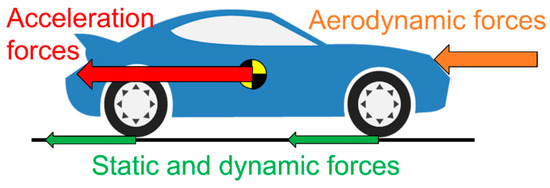
Figure 3.
Forces applied to the vehicle.
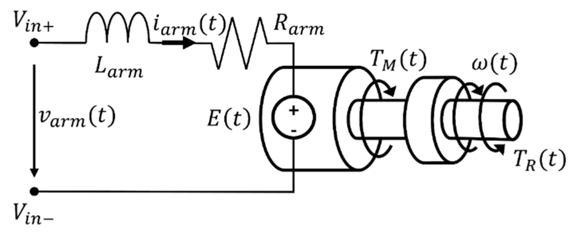
Next, the electric motor model is developed. This motor transforms the electric power into mechanic power in the motor shaft. The DC motor is chosen to explain the procedure step-by-step, although other types of electric motors could be chosen using the same procedure.
Figure 4 shows the model of the electric motor, being ω(t) the angular speed of the wheels (rad/s), TM(t) the motor torque (N·m) on the wheels, iarm(t) the current that goes through the rotor (A) and varm(t) the voltage between the motor connections (V). Rarm, Larm, and E(t) are, respectively, the electrical resistance (Ω), inductance (H), and counter-electromotive force (V) of the electric motor.
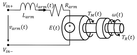
Figure 4.
DC motor model.
The equations of a DC motor are (13) and (14) where K1 and K2 are constant parameters of the motor and, ωmot(t) and Tmot(t) are the angular speed and torque of the DC motor. The electric flux ϕ is assumed constant, which lets replacing K1 and K2, for Kω and KT, which are the speed constant (V/(rad/s)) and the torque constant (N·m/A).
The ratio between the motor shaft and the wheel shaft, rt, allows obtaining the motor torque, TM(t), and the angular speed of the wheel, ω(t). Replacing (15) and (16) into (13) and (14) derives in (17) and (18), which includes the efficiency of the vehicle transmission system and motor, ηT.
The Equation (19) describes the DC electric motor model. On the other hand, in steady-state, TR(t) has to be the same as the motor torque TM(t) that moves the vehicle, as can be seen in (20). Therefore, the Equations (17), (18), (19) and (20) are the four basic equation used to represent a DC electric motor.
Summarizing, the electrical and mechanical equations of the electric motor are (17), (18), (19) and (12). In the model developed, two considerations are assumed, flat terrain and the linear friction coefficient.
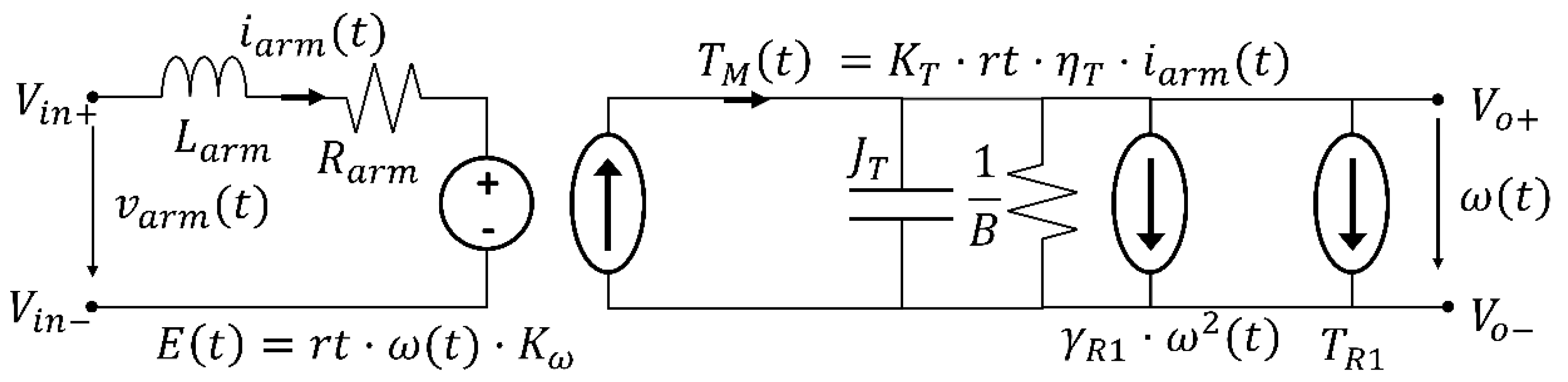
The addends of (12) are shortened in (21). Then, the equivalent circuit of the electric motor is shown in Figure 5.
where:

Figure 5.
Vehicle and electric motor equivalent circuit.
Equation (21) can be interpreted as an electric circuit, where TM(t) can be interpreted as a current, as shown in Figure 5.
3. Control Loop Design
A control circuit is designed with a speed outer loop and a current inner loop to control the motor operation. The vehicle and motor small-signal model must be obtained to achieve this design.
3.1. Vehicle and Motor Small-Signal Model
3.1.1. Vehicle Small-Signal Model
The small-signal model of the vehicle and the motor is obtained by linearizing the terms included in (21) at a working point W, which is the angular speed of the wheels. Concerning the notation, henceforth, the terms â is a perturbation of a variable a. To obtain the linearization of the acceleration torque at W, (26) is replaced in (21):
which gives (27):
where (27) is composed of the motor torque at the working point W, , and the perturbation of the motor torque, , defined in (28) and (29) respectively:
In (28), dW/dt = 0, because W is not a function of time. In (29), is neglected because the terms of the second degree or higher are not considered. Therefore, the motor torque can be expressed, as shown in (30):
Finally, applying the Laplace transformation to (29) gives (31):
where JT and Rol are defined in (22) and (32), considering (24) and (25):
3.1.2. Electric Motor Small-Signal Model
Substituting Equation (17) in (19) and repeating the previously applied procedure gets:
Moreover, proceeding likewise, Equations (17) and (18) gives:
The Laplace transformation of (33), (34) and (35) are (36), (37) and (38), respectively.
Finally, the Equations (31), (36), (37) and (38) give the blocks diagram shown in Figure 6.
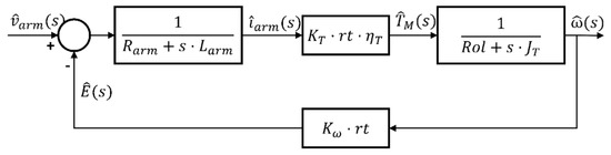
Figure 6.
Block diagram of the small-signal model of both DC motor and vehicle.
3.2. Vehicle and Motor Control Loop
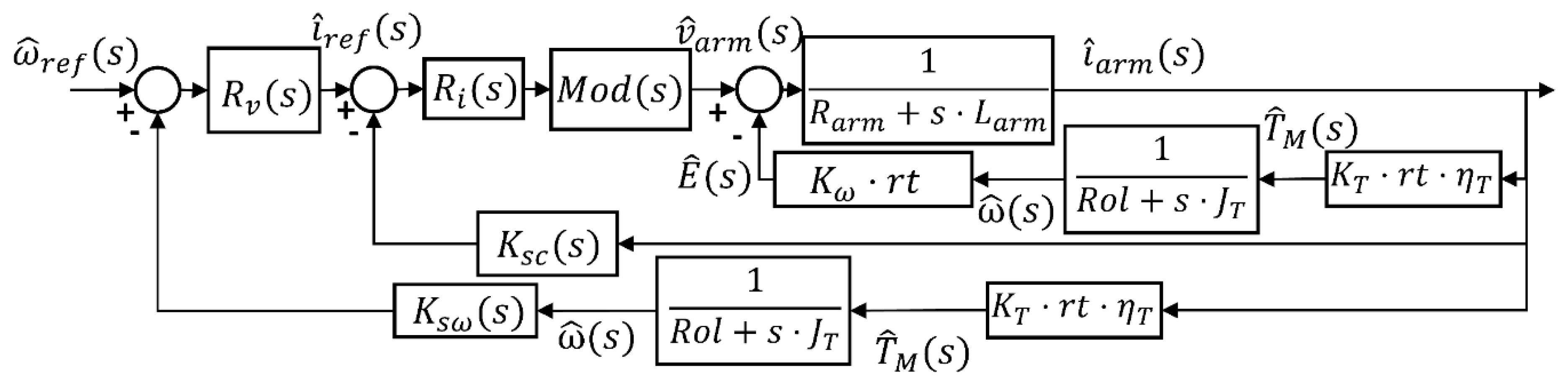
The control loop together with the blocks diagram explained in Figure 2 and Figure 6 is shown in Figure 7. Ri(s) is the transfer function of the current compensator, Mod(s) includes both the modulator and the motor drive power stage, and Rv(s) is the transfer function of the speed compensator. Finally, the terms Ksc(s) and Ksω(s) are the gain related to the internal current loop sensor and external speed loop sensor, respectively. The reference signal is the driving profile, ωref(s).
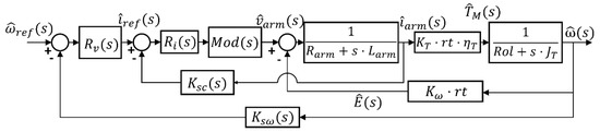
Figure 7.
Block diagram of the small-signal model of DC motor and vehicle together with the control loops.
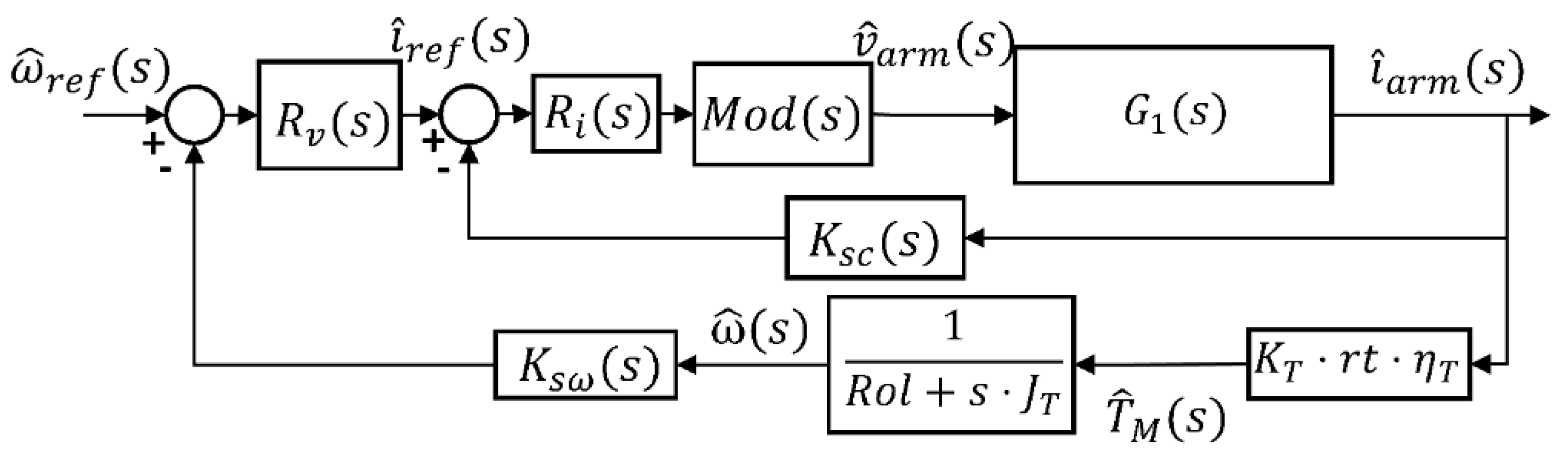
The next step is to simplify the blocks diagram shown in Figure 7. First, the inner loops must be grouped. To achieve that, the blocks of the right side are shifted as shown in Figure 8.

Figure 8.
Block diagram of the modified small-signal model.
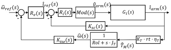
Figure 9.
Block diagram of the small-signal model modified.
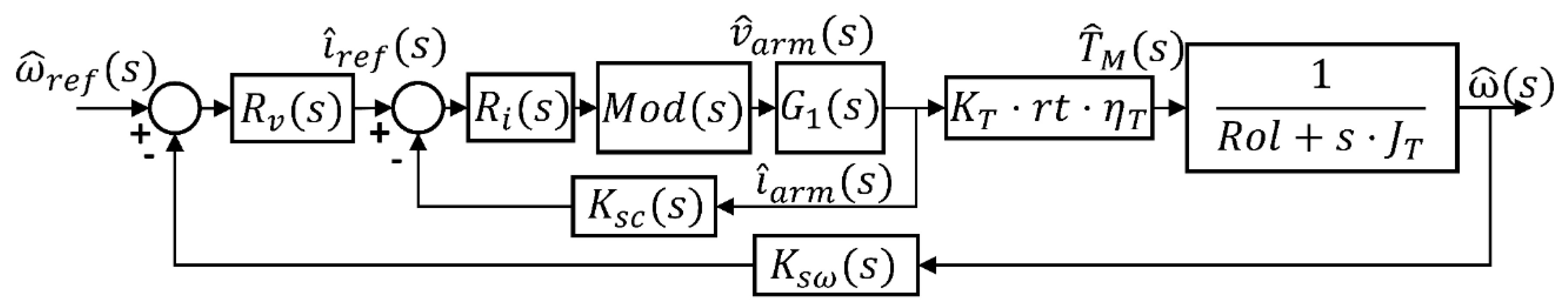
Finally, the two blocks displaced before, now go back to the initial position, as shown in Figure 10.

Figure 10.
Simplified block diagram with inner and outer loops.
Afterward, the transfer function of the current open-loop Ti(s) must be calculated to design the current compensator Ri(s).
Next, the inner loop is simplified in Figure 11, where BCi(s) is the closed-loop transfer function of the current inner loop (41).
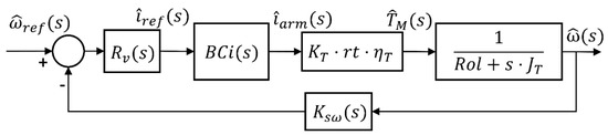
Figure 11.
Block diagram with a simplified inner loop.
From the block diagram shown in Figure 11, the transfer function of the speed open loop Tω(s) can be calculated to design the speed compensator Rv(s).
Based on the Equations (40) and (42), the inner loop compensator and the outer loop compensator can be obtained.
As an example, the data to calculate both compensators, which are obtained using the design software SmartCtrl® (version, manufacturer, city, state abbreviation if USA and Canada, Country) [25], are shown in Table 1. In this case, the gain of the current loop Ksc(s) and speed loop Ksω(s) are assumed constant. The vehicle and motor data are summarized in Table 2 and Table 3, shown in Section 4.

Table 1.
Motor-vehicle compensators data.
Table 2.
Vehicle data. Reproduced with permission from [26].
Table 3.
Electric motor data.
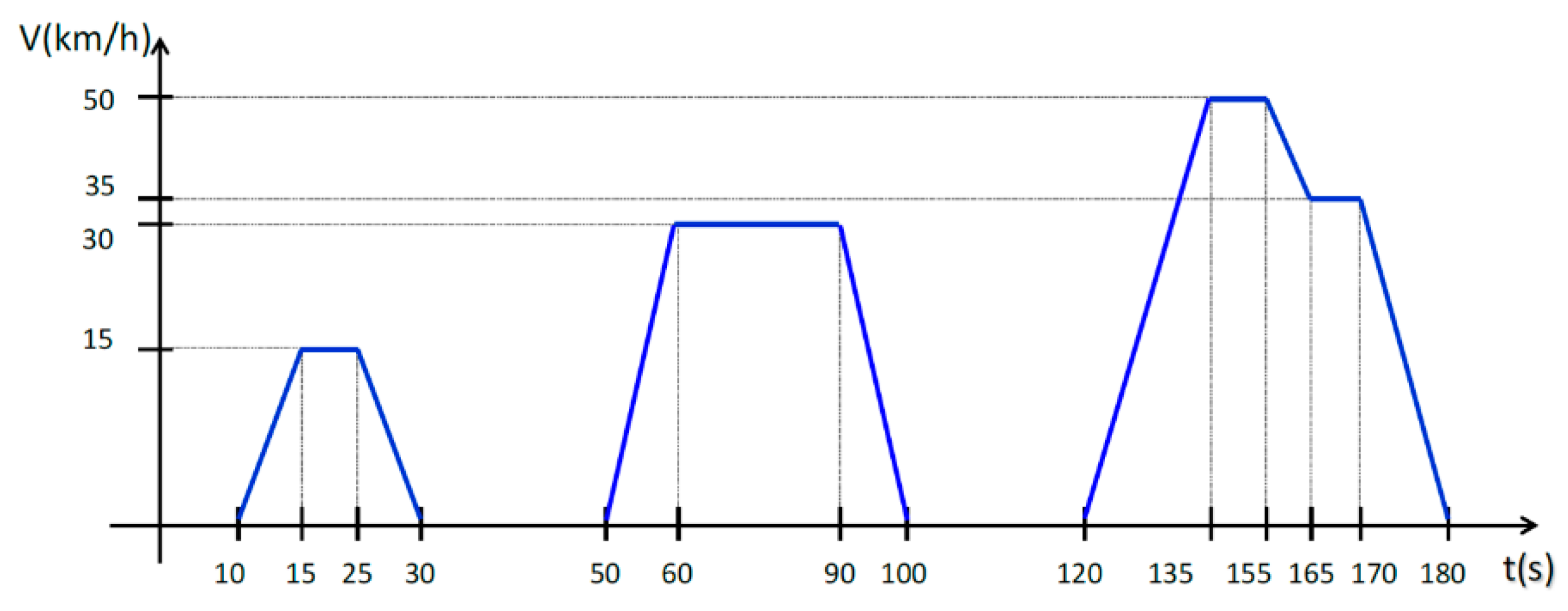
The driving profile shown in Figure 12 is used to evaluate the designed control. It corresponds to a European driving profile, ECE-15, applied to light vehicles.

Figure 12.
Driving profile ECE-15.
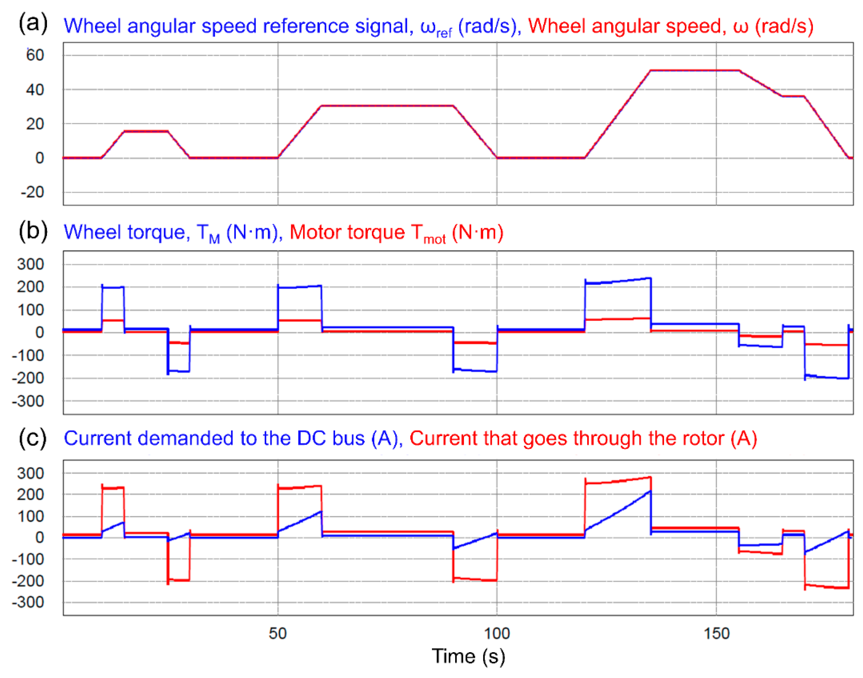
Figure 13 shows the results of applying the ECE-15 driving profile, shown in Figure 12, to the motor-vehicle system. Figure 13a shows the wheel angular speed that must be achieved, ωref, and the simulated, ω. Figure 13b shows both the torque in the wheel, TM, and the torque in the motor, Tmot. The difference between them is due to the ratio between the motor shaft and the wheel shaft, rt. Figure 13c shows the current through the rotor, iarm, and the demanded current to the DC bus. As the motor input voltage is lower than the DC bus voltage, the current through the rotor is higher than the current demanded to the DC bus.
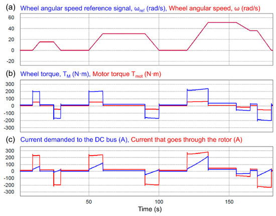
As can be seen in Figure 13, the speed increments or decrements imply positive or negative motor torque, which involve positive or negative currents in the rotor. Thus, using the carried out modeling a driving profile can be transformed into a current profile that has to be supplied by the power distribution system from the DC bus.
4. Electrical Impedance Analysis
In this section, the small-signal input impedance of the system composed of the vehicle, the electric motor, the motor drive, and the filter is obtained. This input impedance can affect system stability.
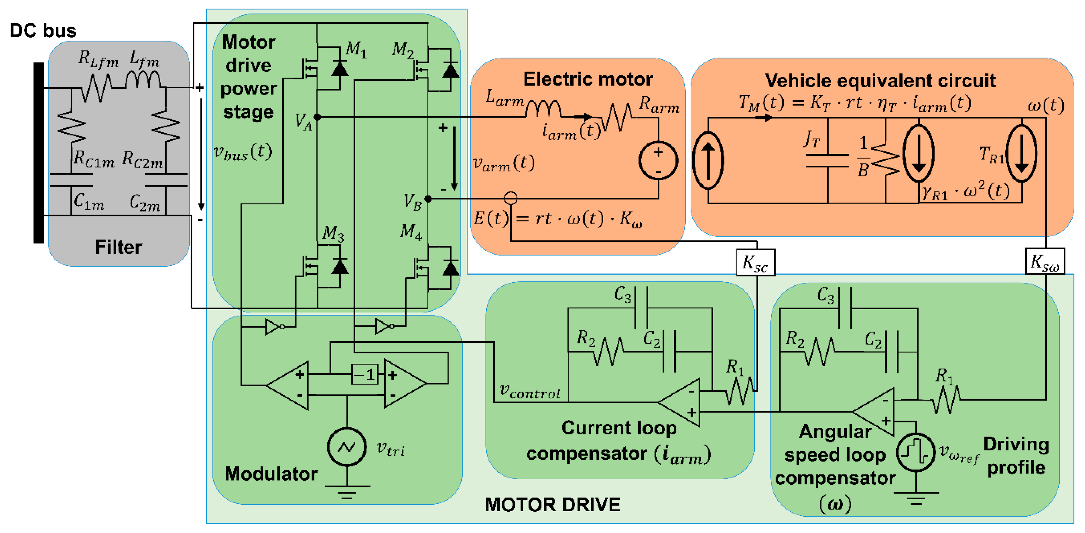
Figure 14 shows the analyzed system, divided into three main blocks. The first one is the motor drive that enables the vehicle to run and brake, which includes an inner loop to control iarm and outer loop to control ω. The second one is the input circuit of the electric motor (shown as an Electric motor). Finally, the last one is the vehicle equivalent circuit. In addition, Figure 14 shows the input filter of the motor drive-electric motor-vehicle system.
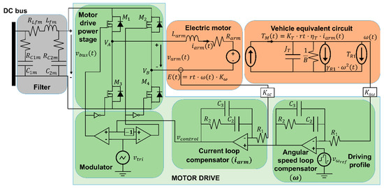
Figure 14.
A system composed of the vehicle, electric motor, motor drive, and filter.
The outer loop compares the angular speed of the motor, ω(t), with the reference signal, which depends on the driving profile. The inner loop uses the output of the outer loop as a reference signal and generates the modulator input signal.
In this analysis, it is assumed that the motor speed dynamics is much slower than the motor current dynamics. This hypothesis allows us to assume that the counter-electromotive force E(t) is constant. Therefore, the reference signal of the current loop, which is the output of the speed loop, can also be assumed constant. Taking this into account, there is no dependence between the electric motor circuit and the vehicle equivalent circuit from the point of view of the current loop operation.
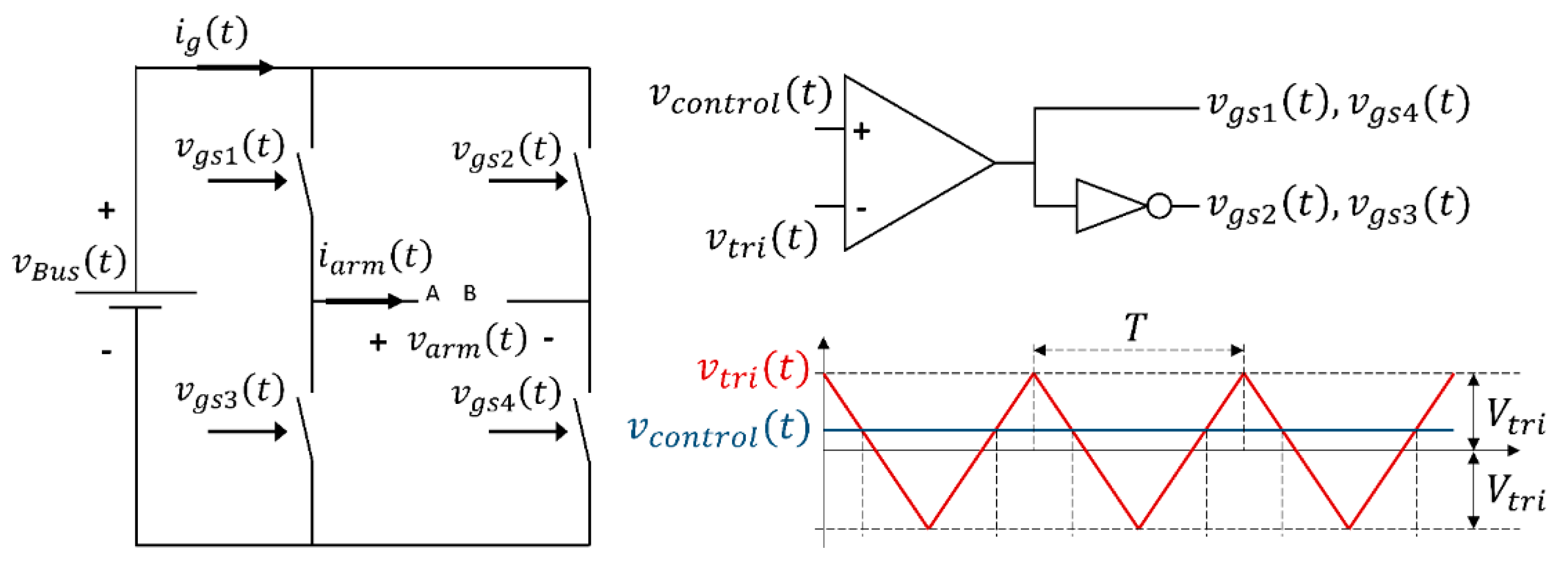
The averaged model of the motor drive shown in Figure 15 is calculated to obtain the electric motor impedance, where vcontrol(t) is the output signal of the inner loop compensator, and vtri(t) is the modulator signal.
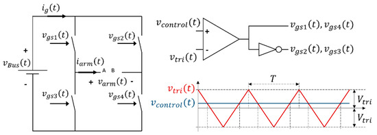
Figure 15.
Motor drive and the pulse-width modulation.
The relation between the bus power, PBus(t), and the motor power, Pmot(t), is given by (43), where ηDF is the efficiency of both motor drive and filter (not included Figure 5):
where Pmot(t) and PBus(t) are:
The averaged output voltage vAB and the averaged input current ig are:
where d is the duty cycle, defined as:
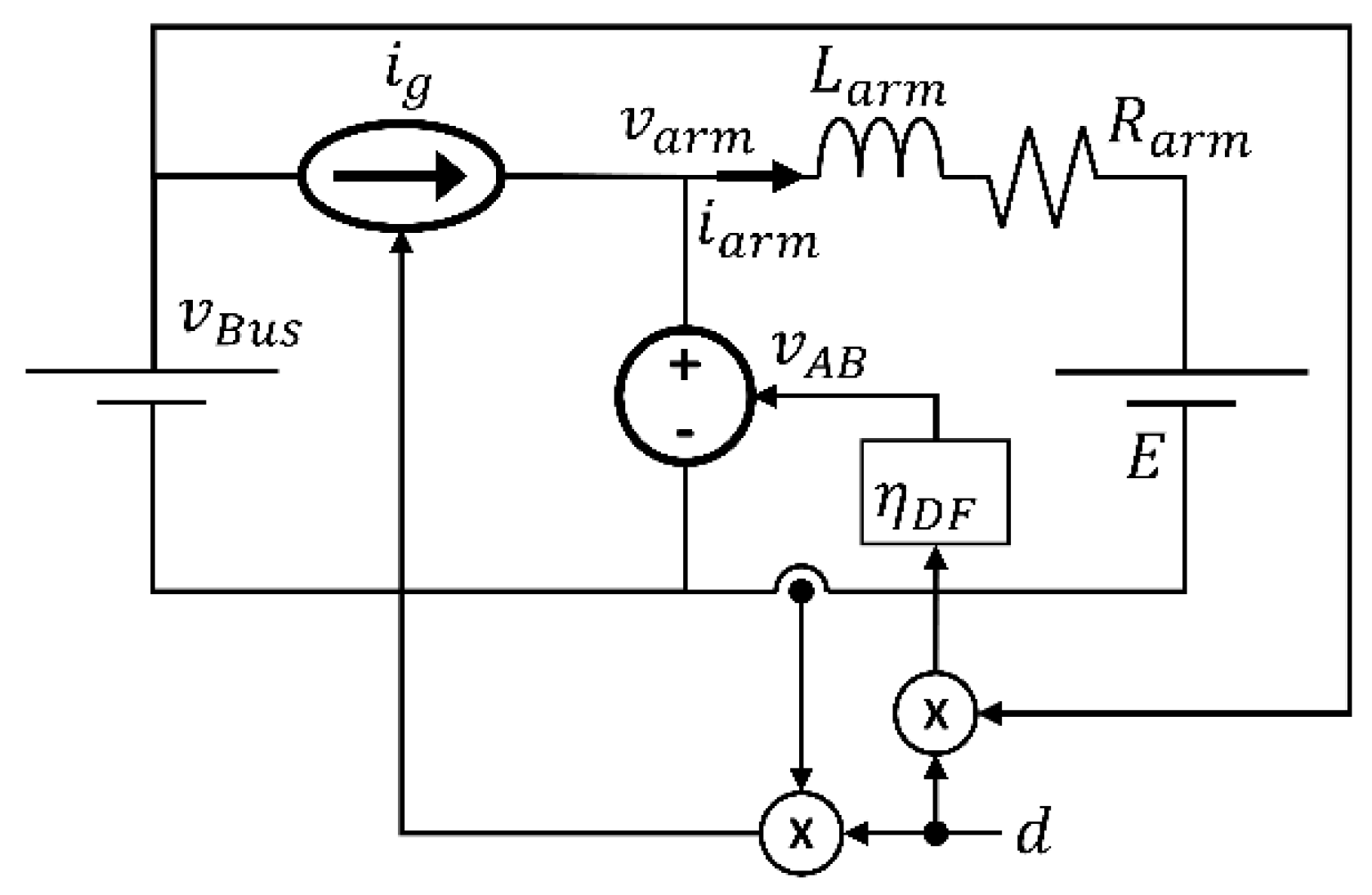
Afterward, once the motor drive averaged model is known, the motor drive-electric motor-vehicle system averaged model can be obtained. The model, shown in Figure 16, uses the previously claimed assumptions.

Figure 16.
Averaged model of the motor drive-electric motor-vehicle system, including the inner current loop.
The obtained model is nonlinear. Therefore, the Equations (46) and (47) must be linearized at the working points Vcontrol, VBus, and Iarm.
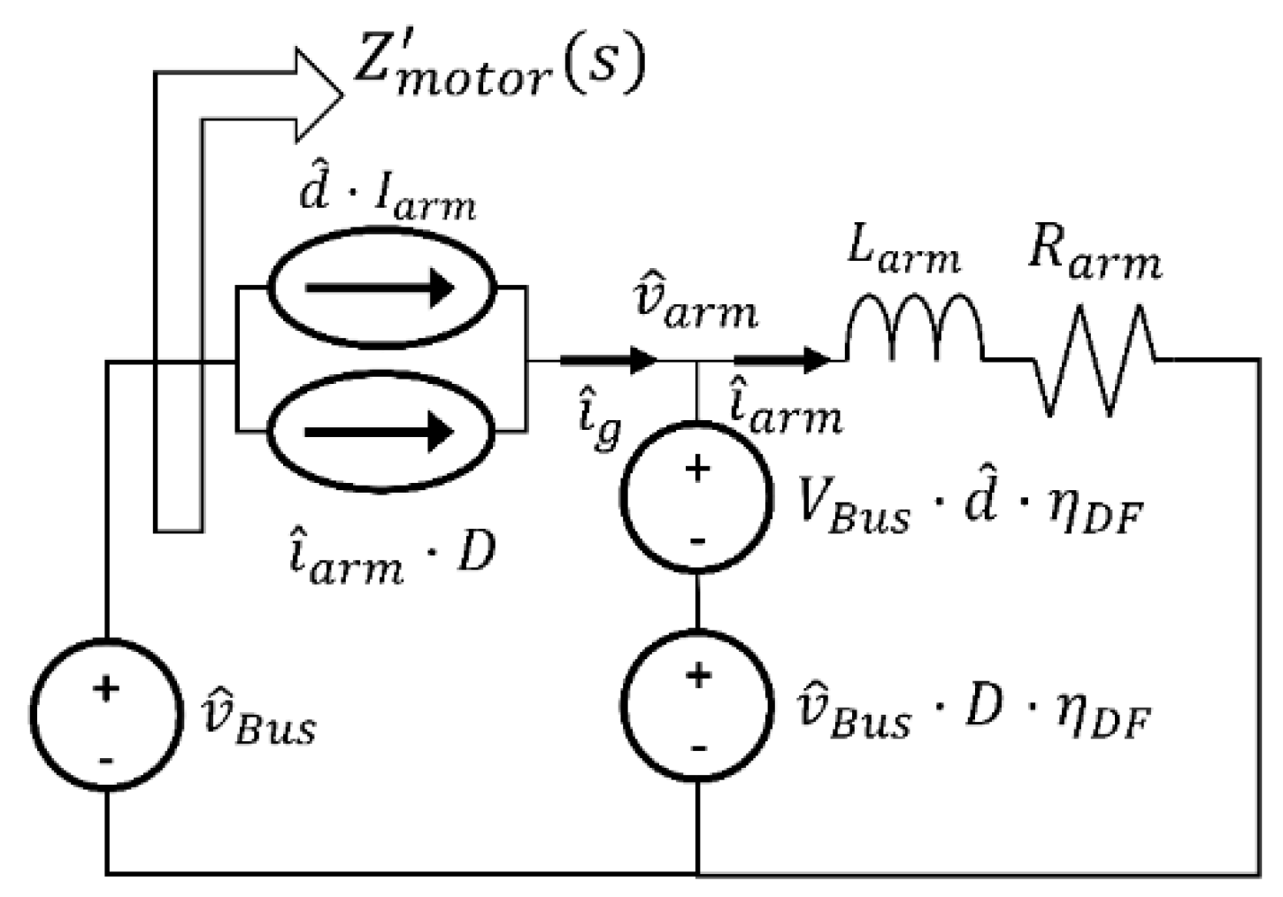
Figure 17 depicts the small-signal model of the motor drive-electric motor-vehicle system without the control loop.

Figure 17.
The small-signal model of the motor drive-electric motor-vehicle system.
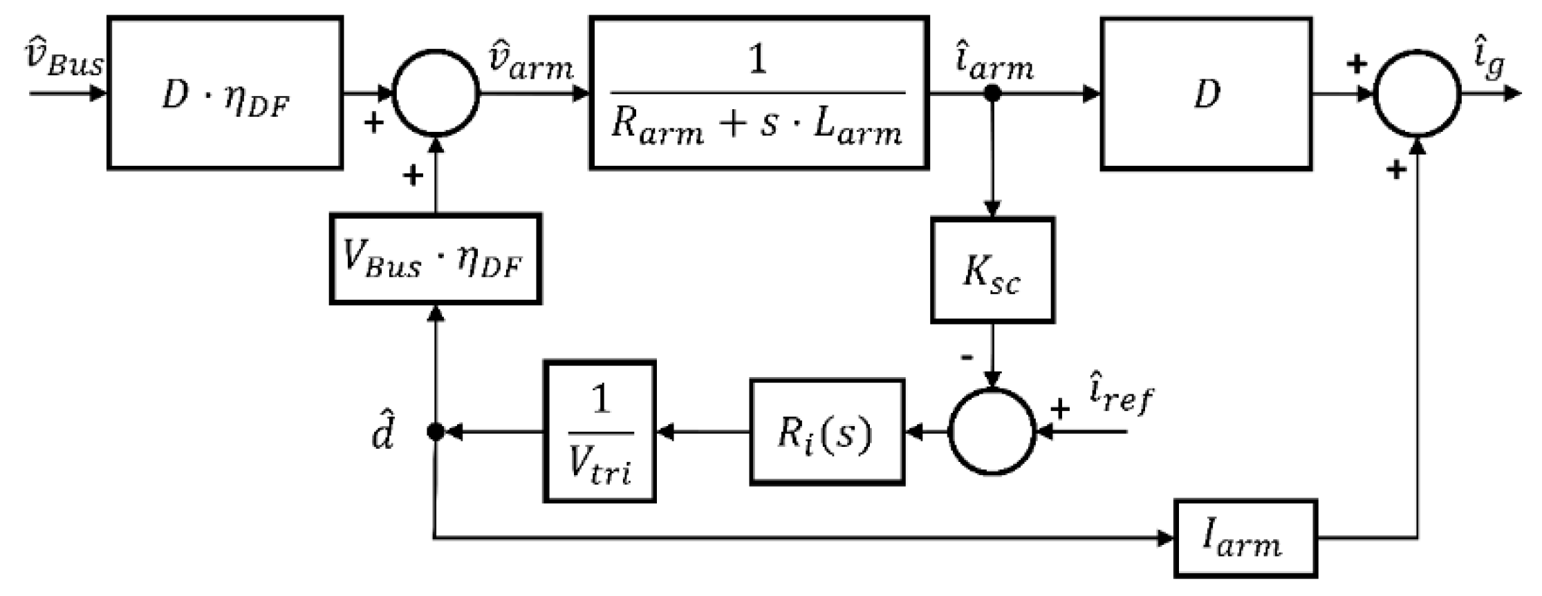
In Figure 17, Z’motor(s) is the motor drive-electric motor-vehicle system input impedance. The block diagram of the motor drive-electric motor-vehicle system small-signal model, together with the control loop, is shown in Figure 18. The equations used to obtain the block diagram are (36), (49), (50), where the counter-electromotive force E(t) is surmised constant.
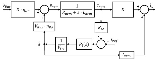
Figure 18.
Block diagram of the motor drive-electric motor-vehicle system, including the inner control loop.
As stated above, the reference of the current is assumed constant. This way, a simplified model is shown in Figure 19.
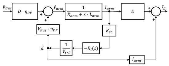
Figure 19.
Simplified block diagram of the motor drive-electric motor-vehicle system with the inner control loop and without current reference signal variation.
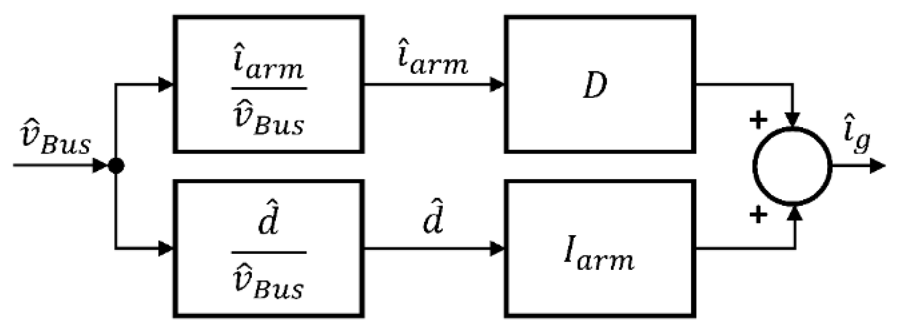
As the goal is to obtain the transfer function that relates the current that goes through the rotor iarm, the duty cycle d, and bus voltage vBus, the blocks diagram shown in Figure 20 can be considered.

Figure 20.
Modified block diagram of the motor drive-electric motor-vehicle system with the inner control loop.
The two diagrams placed on the left side in Figure 20 are named Giv(s) and Gdv(s). Their transfer functions appear in (51) and (52). They are obtained from the blocks diagram in Figure 19.
where:
Replacing (53) in (52) gives:
Once Giv(s) and Gdv(s) are known, the input impedance of the motor drive-electric motor-vehicle system represented in Figure 17, Z’motor(s), can be obtained using the block diagram shown Figure 20.
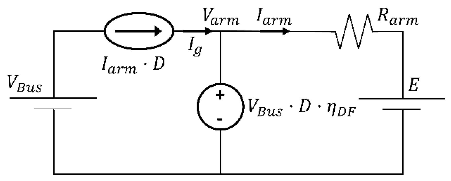
Last, to obtain the input impedance, the working points of D, and Iarm must be calculated. To achieve it, the steady-state circuit shown in Figure 21 is used together with the electric motor mechanical equations.

Figure 21.
The steady-state equivalent circuit of the motor drive-electric motor-vehicle system.
E is defined in (58), where W is the angular speed at the working point:
On the other hand, using the motor torque Equation (59), Iarm is derived in (60).
Finally, D can be obtained, as shown in (61).
The vehicle and electric motor data must be known to develop the impedance analysis. The data used are shown in Table 2 and Table 3, which correspond to a light vehicle and an electric motor model GEM 5BC449JB6007.
If the electric motor allows energy recovery, the motor has two modes. In motor mode, the vehicle is accelerating, and thus, the motor demands energy from the system. In generator mode, the vehicle is decelerating, and therefore, the motor supplies energy to the system. In both modes, the model and behavior of the motor drive, the electric motor, and the control loops are the same. Thus the impedance calculation procedure remains equal.
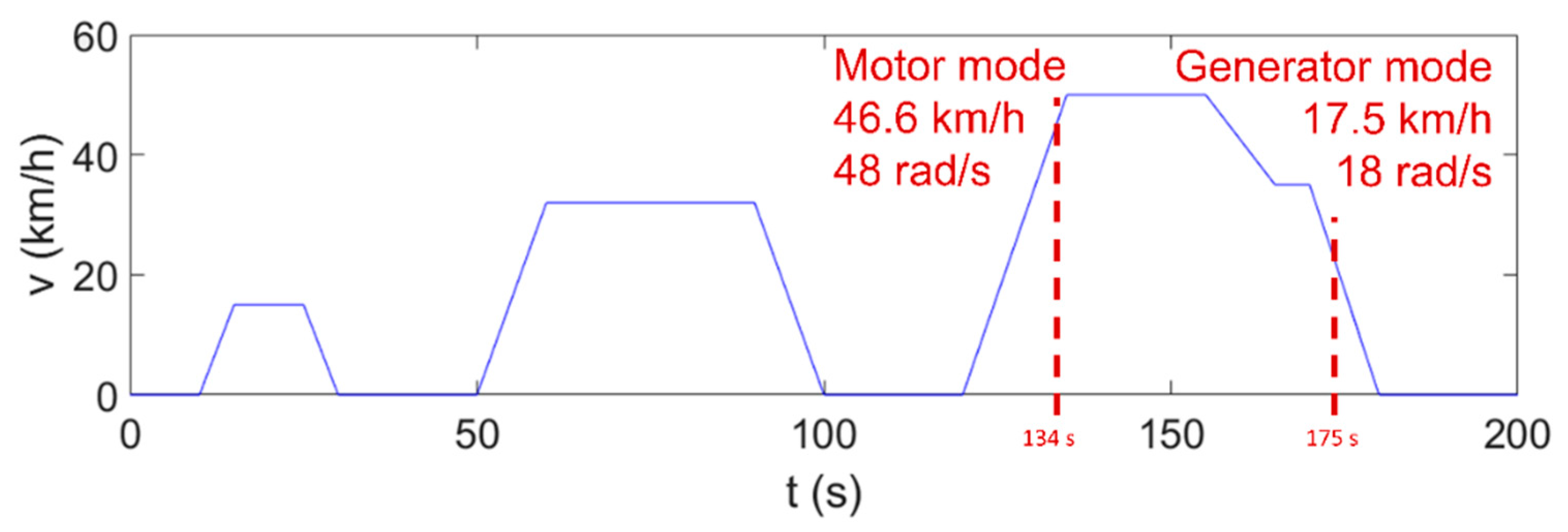
The working point W is chosen using a standard driving profile. This profile depends on the vehicle and the driving pattern used. As commented before, the driving profile chosen is the Urban Driving Cycle (UDC or ECE-15), which represents the typical driving conditions of busy European cities, with 50 km/h maximum speed. The working points in both motor and generator mode are shown in Figure 22, and the corresponding data is shown in Table 4.
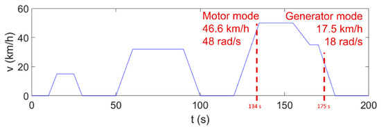
Figure 22.
Working points selected in the ECE-15 driving profile to evaluate the input impedance of the motor drive-electric motor-vehicle system in both motor and generator mode.
Table 4.
The working point in motor and generator mode.
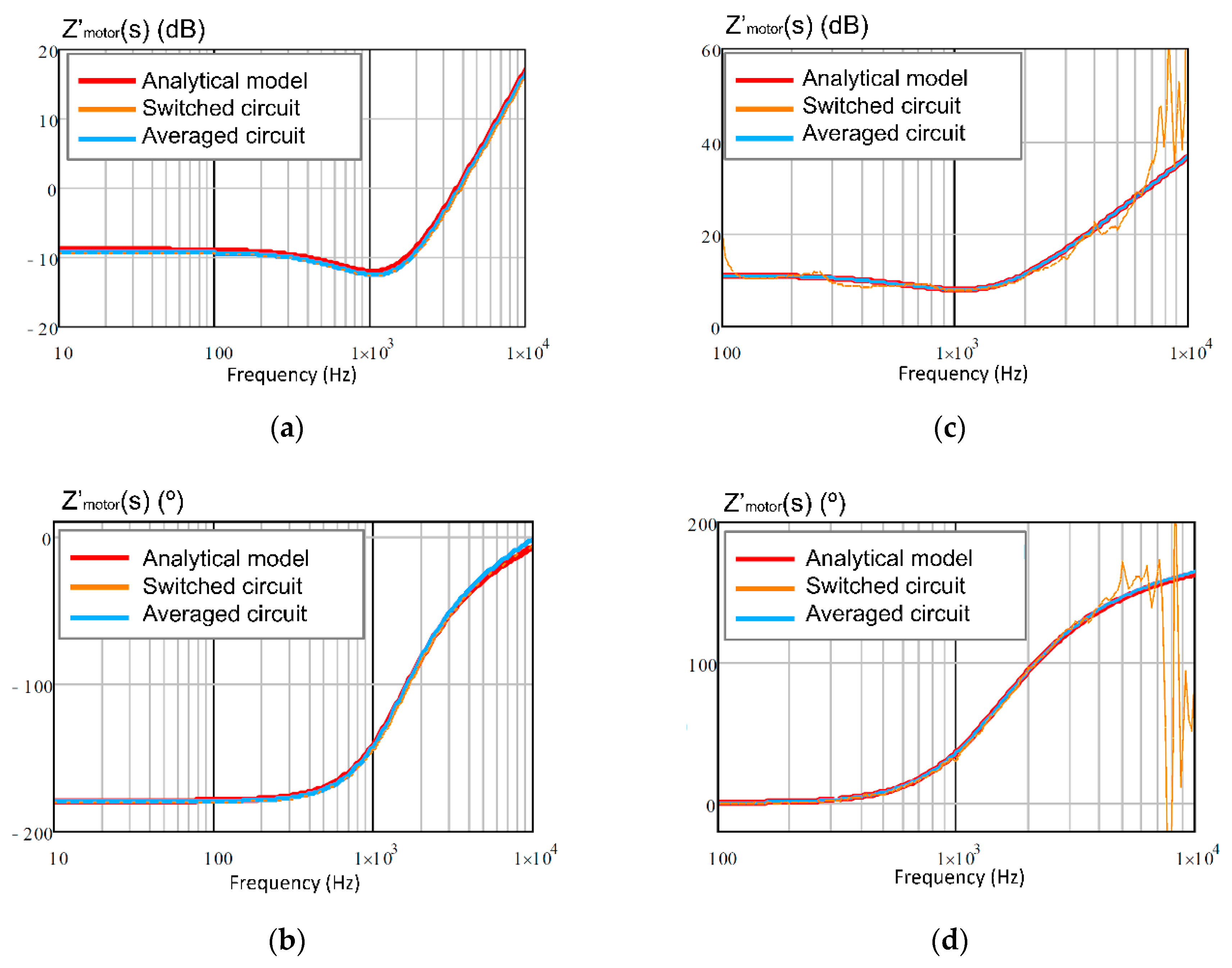
Next, the frequency response of the small-signal input impedance obtained by three different methods are shown in Figure 23a,b for motor mode, and in Figure 23c,d for generator mode. The first method is the frequency response obtained with the averaged circuit, shown in Figure 16, by using Equations (46) and (47). The second method is the frequency response obtained from the switched circuit, shown in Figure 14. The third method is the frequency response obtained from the small-signal analytical model, shown in Figure 17, by using Equations (49) and (50).
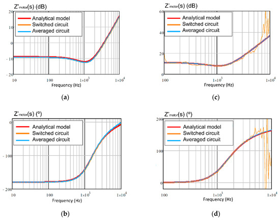
Figure 23.
Frequency response of the small-signal input impedance, Z’motor(s), of the motor drive-electric motor-vehicle system in both motor mode, (a) gain and (b) phase; and generator mode, (c) gain and (d) phase.
In both motor mode and generator mode, the input impedance of the converter presents two parts. Below 1 kHz, the impedance can be represented as a resistance, and above this frequency the input impedance has inductive behavior. Note that the Z’motor(s) does not include the typical input capacitor, which in this case belongs to the filter block. The only difference between motor and generator mode is the phase value, so the motor mode has negative impedance, and the generator mode has positive impedance.
The mean absolute percentage error (MAPE) is measured using the natural impedance values (Ω) instead of dB. On the one hand, by comparing the switched circuit frequency response and the averaged circuit frequency response the MAPE reaches a value of 2.17%. On the other hand, by comparing the small-signal analytical model frequency response and the averaged circuit frequency response, the higher MAPE value is 3.98%.
However, as the transmission of high-frequency ripples to the system must be limited, a filter is placed between the motor drive and the DC bus, as Figure 14 illustrates. Therefore, the impedance including the filter, Zmotor(s), shown in Figure 24, must be obtained.
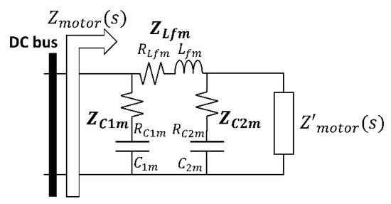
Figure 24.
The input impedance of the motor drive-electric motor-vehicle system, including the input filter.
Then, Zmotor(s) is defined in (62):
Being ZM1(s) and ZM2(s):
The goal of the filter is to reduce the propagation of the high-frequency switching ripple of the motor drive-electric motor-vehicle system towards the rest of the powertrain. The data related to the filter are shown in Table 5.
Table 5.
Input filter data of the motor drive-electric motor-vehicle system.
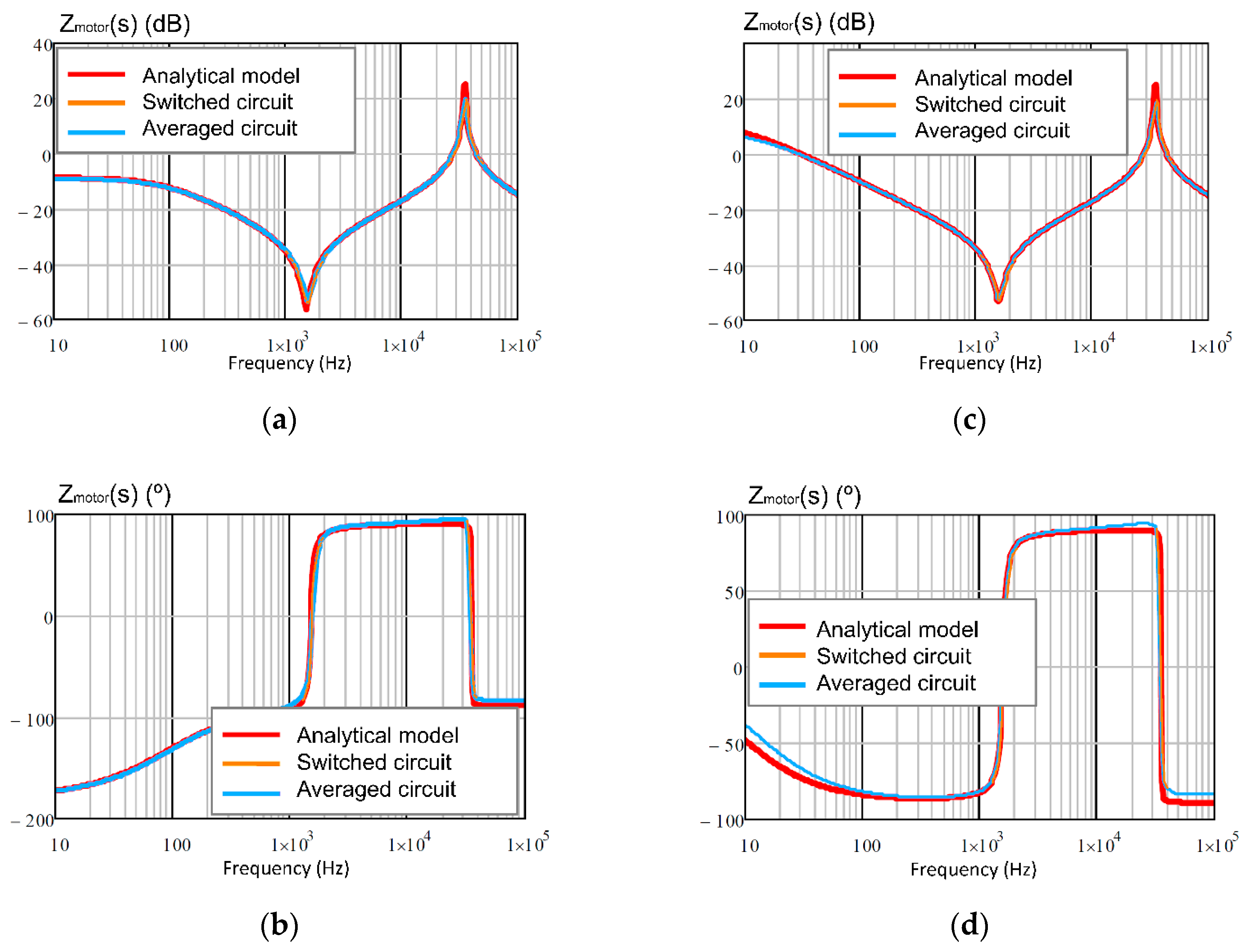
The frequency responses of the small-signal input impedance, Zmotor(s), are shown in Figure 25a,b for motor mode, and in Figure 25c,d for generator mode. Figure 25 shows the averaged circuit, shown in Figure 16, using Equations (46) and (47); the switched circuit, shown in Figure 14; and the small-signal analytical model, shown in Figure 17, using Equations (49) and (50).
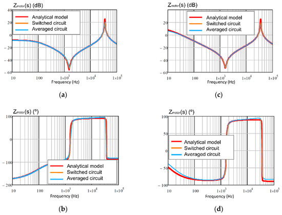
Figure 25.
Frequency response of the small-signal input impedance, Zmotor(s), of the motor drive-electric motor-vehicle system in both motor mode, (a) gain and (b) phase; and generator mode, (c) gain and (d) phase.
In both modes, a resonance and an anti-resonance can be observed. The resonance is imposed by Lfm and C2m, 1.59 kHz, and the anti-resonance depends on the Lfm and C1m, 35.58 kHz.
At low frequency, the filter does not affect, but above 159 Hz the input impedance is determined by the input filter.
The higher MAPE obtained by comparing the switched circuit frequency response and the averaged circuit frequency response is 2.43%. On the other hand, the MAPE reaches a maximum value of 4.6% when comparing the small-signal analytical model frequency response and the averaged circuit frequency response.
5. Conclusions
This paper develops, step-by-step and in detail, the main analyses that must be addressed to obtain a complete electric model of a light hybrid electric vehicle propulsion system, as well as the input impedance expressions necessary to evaluate the system stability.
The complete electric model of a light hybrid electric vehicle propulsion system includes the most important parameters that affect the relationship between the vehicle speed and the energy demanded from the power sources. These parameters are the vehicle mass, the radius and the mass of the wheels, the aerodynamic profile of the vehicle, the electric motor, the motor drive, and the motor and transmission system efficiency, among others.
In addition, the paper shows the procedure to obtain the analytical expression of the small-signal model of the complete analyzed system compound by the vehicle, the electric motor, the motor drive (including two control loops), and the input filter. The inner and outer open-loop gains, which determine the current and speed compensator included in the motor drive, has been obtained from the small-signal model. These loops provide good stability and dynamic response, which helps the motor to achieve the desired speed. With this information, the simulation results show the relationship among speed vehicle, the wheel torque, the electric motor torque, the current demanded by the DC bus, and the electric motor current, in closed-loop.
From the system stability viewpoint, this paper shows the procedure to calculate the small-signal input impedance of the motor drive-electric motor-vehicle-filter system. By using this procedure, the general expression of the input impedance has been obtained. These analytical results have been compared with the input impedance obtained by PSIM®, from the simulation of the complete average circuit and the complete switched circuit. All results are consistent, demonstrating the accuracy of the obtained analytical expressions. This input impedance is especially useful to get the stability of the entire system.
Therefore, this paper provides a complete propulsion system model simple enough to enable the system simulation, once the main components have been designed, with the aim of achieving the system stability and enough transient response.
Author Contributions
C.R. did theoretical analysis, derivation, system implementation, simulation, data processing, and wrote the first original draft paper. A.L. contributed to theoretical analysis and supervision. A.B. was responsible for funding acquisition, supervision, and administration, his contribution was related to the theoretical analysis, data analysis, and the paper reviewing and editing. A.M.-L. helped to write the last version of the draft paper. I.Q. helped with the derivation and to write a first original draft paper.
Funding
This research was funded by the Spanish Ministry of Economy and Competitiveness and ERDF, grant number DPI2014-53685-C2-1-R.
Acknowledgments
This work has been partially supported by the Spanish Ministry of Economy and Competitiveness and FEDER (ERDF), through the research project “Storage and Energy Management for Hybrid Electric Vehicles based on Fuel Cell, Battery and Supercapacitors"—ELECTRICAR-AG- (DPI2014-53685-C2-1-R).
Conflicts of Interest
The authors declare no conflict of interest.
References
- The Electric Vehicle World Sales Database Global Plug-in Sales for Q1-2018. Available online: http://www.ev-volumes.com/country/total-world-plug-in-vehicle-volumes/ (accessed on 24 September 2019).
- Bunsen, T.; Cazzola, P.; Gorner, M.; Paoli, L.; Scheffer, S.; Schuitmaker, R.; Teter, J. Global EV Outlook 2018; International Energy Agency: Paris, France, 2018; p. 78. [Google Scholar] [CrossRef]
- Wei, Z.; Xu, J.; Halim, D. HEV power management control strategy for urban driving. Appl. Energy 2017, 194, 705–714. [Google Scholar] [CrossRef]
- Feng, X.; Lewis, M.; Hearn, C. Modeling and Validation for Zero Emission Buses. In Proceedings of the 2017 IEEE Transportation Electrification Conference and Expo (ITEC), Chicago, IL, USA, 22–24 June 2017; pp. 501–506. [Google Scholar] [CrossRef]
- Kuralay, N.S.; Colpan, C.O.; Karao, M.U. The effect of gear ratios on the exhaust emissions and fuel consumption of a parallel hybrid vehicle powertrain. J. Clean. Prod. 2019, 210, 1033–1041. [Google Scholar] [CrossRef]
- Feroldi, D.; Carignano, M. Sizing for fuel cell/supercapacitor hybrid vehicles based on stochastic driving cycles. Appl. Energy 2016, 183, 645–658. [Google Scholar] [CrossRef]
- Jithin, T.J.; Prasanth, P.; Gautam, V.; Meheranusha, V.; Kumaravel, S.; Ashok, S. A Sensitivity Analysis on Performance of a Typical Single Axle Battery Electric Vehicle. In Proceedings of the 2018 International Conference on Power, Energy, Control and Transmission Systems (ICPECTS), Chennai, India, 22–23 February 2018; pp. 158–164. [Google Scholar]
- Fiori, C.; Ahn, K.; Rakha, H.A. Microscopic series plug-in hybrid electric vehicle energy consumption model: Model development and validation. Transp. Res. Part D 2018, 63, 175–185. [Google Scholar] [CrossRef]
- Geng, S.; Meier, A.; Schulte, T. Model-Based Optimization of a Plug-In Hybrid Electric Powertrain with Multimode Transmission. World Electr. Veh. J. 2018, 9, 12. [Google Scholar] [CrossRef]
- Vafaeipour, M.; El Baghdadi, M.; Verbelen, F.; Sergeant, P.; Mierlo, J. Van Technical Assessment of Utilizing an Electrical Variable Transmission System in Hybrid Electric Vehicles. In Proceedings of the 2018 IEEE Transportation Electrification Conference and Expo, Asia-Pacific (ITEC Asia-Pacific), Bangkok, Thailand, 6–9 June 2018. [Google Scholar] [CrossRef]
- Porru, M.; Serpi, A.; Floris, A.; Damiano, A. Modelling and Real-Time Simulations of Electric Propulsion Systems. In Proceedings of the 2016 International Conference on Electrical Systems for Aircraft, Railway, Ship Propulsion and Road Vehicles & International Transportation Electrification Conference (ESARS-ITEC), Toulouse, France, 2–4 November 2016; pp. 5–10. [Google Scholar] [CrossRef]
- Reeves, K. Validation of a Hybrid Electric Vehicle Dynamics Model for Energy Management and Vehicle Stability Control. In Proceedings of the 2016 IEEE 25th International Symposium on Industrial Electronics (ISIE), Santa Clara, CA, USA, 8–10 June 2016; pp. 849–854. [Google Scholar] [CrossRef]
- Jauch, C.; Bovee, K.; Tamilarasan, S.; Giivenc, L.; Rizzoni, G. Modeling of the OSU EcoCAR 2 vehicle for drivability analysis. IFAC-PapersOnLine 2015, 28, 300–305. [Google Scholar] [CrossRef]
- Li, H.; Hu, X.; Fu, B.; Wang, J.; Zhang, F. Effective optimal control strategy for hybrid electric vehicle with continuously variable transmission. Adv. Mech. Eng. 2019, 11, 1–11. [Google Scholar] [CrossRef]
- Li, H.; Zhou, Y.; Xiong, H.; Fu, B.; Huang, Z. Real-Time Control Strategy for CVT-Based Hybrid Electric Vehicles Considering Drivability Constraints. Appl. Sci. 2019, 9, 2074. [Google Scholar] [CrossRef]
- Pany, P.; Singh, R.K.; Tripathi, R.K. Active load current sharing in fuel cell and battery fed DC motor drive for electric vehicle application. Energy Convers. Manag. 2016, 122, 195–206. [Google Scholar] [CrossRef]
- Valan Rajkumar, M.; Ranjhitha, G.; Pradeep, M.; Pk, M.F.; Kumar, R.S. Fuzzy based Speed Control of Brushless DC Motor fed Electric Vehicle. Int. J. Innov. Stud. Sci. Eng. Technol. 2017, 4863, 2455–4863. [Google Scholar]
- Yang, Z.; Shang, F.; Brown, I.; Krishnamurthy, M. Comprehensive Comparison of Interior Permanent Magnet, Induction and Switched Reluctance Motor Drives for EV and HEV Application. IEEE Trans. Transp. Electrif. 2015. [Google Scholar] [CrossRef]
- Mebarki, N.; Rekioua, T.; Mokrani, Z.; Rekioua, D.; Bacha, S. PEM fuel cell / battery storage system supplying electric vehicle direct Torque Control. Int. J. Hydrog. Energy 2016, 41, 20993–21005. [Google Scholar] [CrossRef]
- Yu, J.; Ma, Y.; Yu, H.; Lin, C. Adaptive fuzzy dynamic surface control for induction motors with iron losses in electric vehicle drive systems via backstepping. Inf. Sci. 2017, 376, 172–189. [Google Scholar] [CrossRef]
- Guo, Q.; Zhang, C.; Li, L.; Gerada, D.; Zhang, J.; Wang, M. Design and implementation of a loss optimization control for electric vehicle in-wheel permanent-magnet synchronous motor direct drive system. Appl. Energy 2017, 204, 1317–1332. [Google Scholar] [CrossRef]
- Guo, D.; Dinavahi, V.; Wu, Q.; Wang, W. Sliding Mode High Speed Control of PMSM for Electric Vehicle Based on Flux-weakening Control Strategy. In Proceedings of the 2017 36th Chinese Control Conference (CCC), Dalian, China, 26–28 July 2017; pp. 3754–3758. [Google Scholar] [CrossRef]
- Sant, A.V.; Khadkikar, V.; Xiao, W.; Zeineldin, H.H. Four-Axis Vector-Controlled Dual-Rotor PMSM for Plug-in Electric Vehicles. IEEE Trans. Ind. Electron. 2015, 62, 3202–3212. [Google Scholar] [CrossRef]
- Dominguez-Navarro, J.A.; Artal-Sevil, J.S.; Pascual, H.A.; Bernal-Agustin, J.L. Fuzzy-logic strategy control for switched reluctance machine. In Proceedings of the 2018 Thirteenth International Conference on Ecological Vehicles and Renewable Energies (EVER), Monte-Carlo, Monaco, 10–12 April 2018; pp. 1–5. [Google Scholar] [CrossRef]
- SmartCtrl 4.0. Available online: https://www.powersmartcontrol.com (accessed on 12 March 2019).
- Raga, C.; Barrado, A.; Miniguano, H.; Lazaro, A.; Quesada, I.; Martin-Lozano, A.; Raga, C.; Barrado, A.; Miniguano, H.; Lazaro, A.; et al. Analysis and Sizing of Power Distribution Architectures Applied to Fuel Cell Based Vehicles. Energies 2018, 11, 2597. [Google Scholar] [CrossRef]
- Powersim PSIM 2015. Available online: https://powersmartcontrol.com/ (accessed on 24 September 2019).


© 2019 by the authors. Licensee MDPI, Basel, Switzerland. This article is an open access article distributed under the terms and conditions of the Creative Commons Attribution (CC BY) license (http://creativecommons.org/licenses/by/4.0/).