Energy and Efficiency Evaluation of Feedback Branch Design in Thermoacoustic Stirling-Like Engines


Abstract
:1. Introduction
2. DeltaEC Model of the TA-SLiCE Prototype
3. Methodology for Design Improvement
3.1. Factors and Response Variable Selection
3.2. Dimensional Reduction ( FFD)
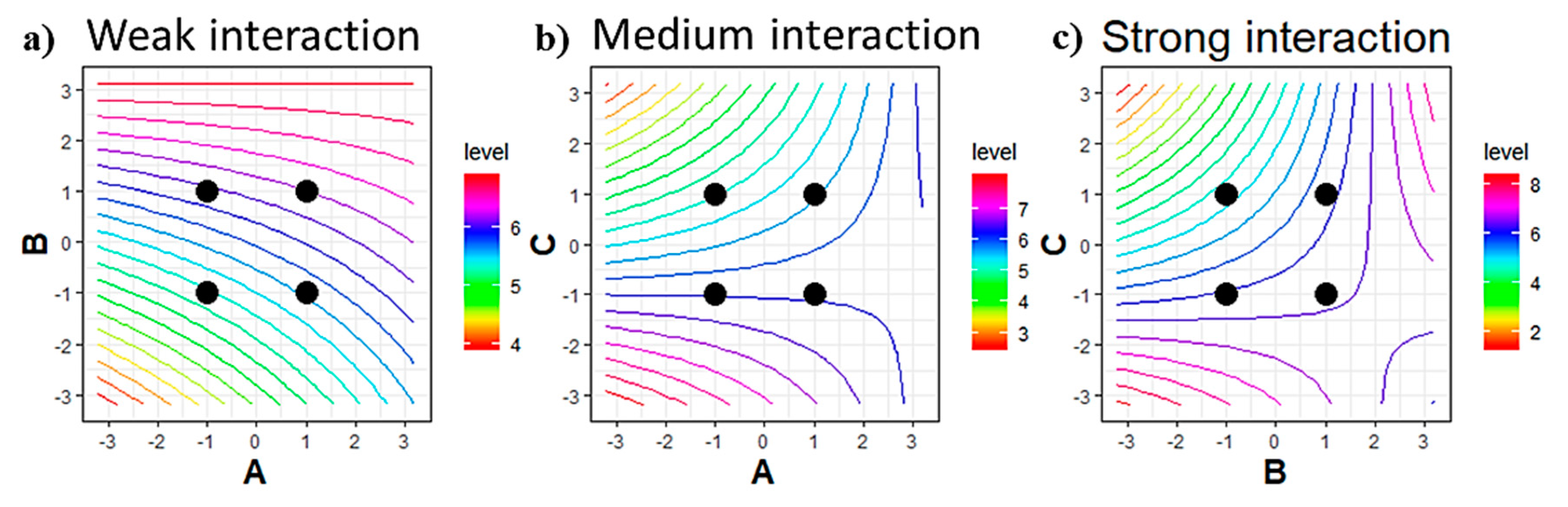
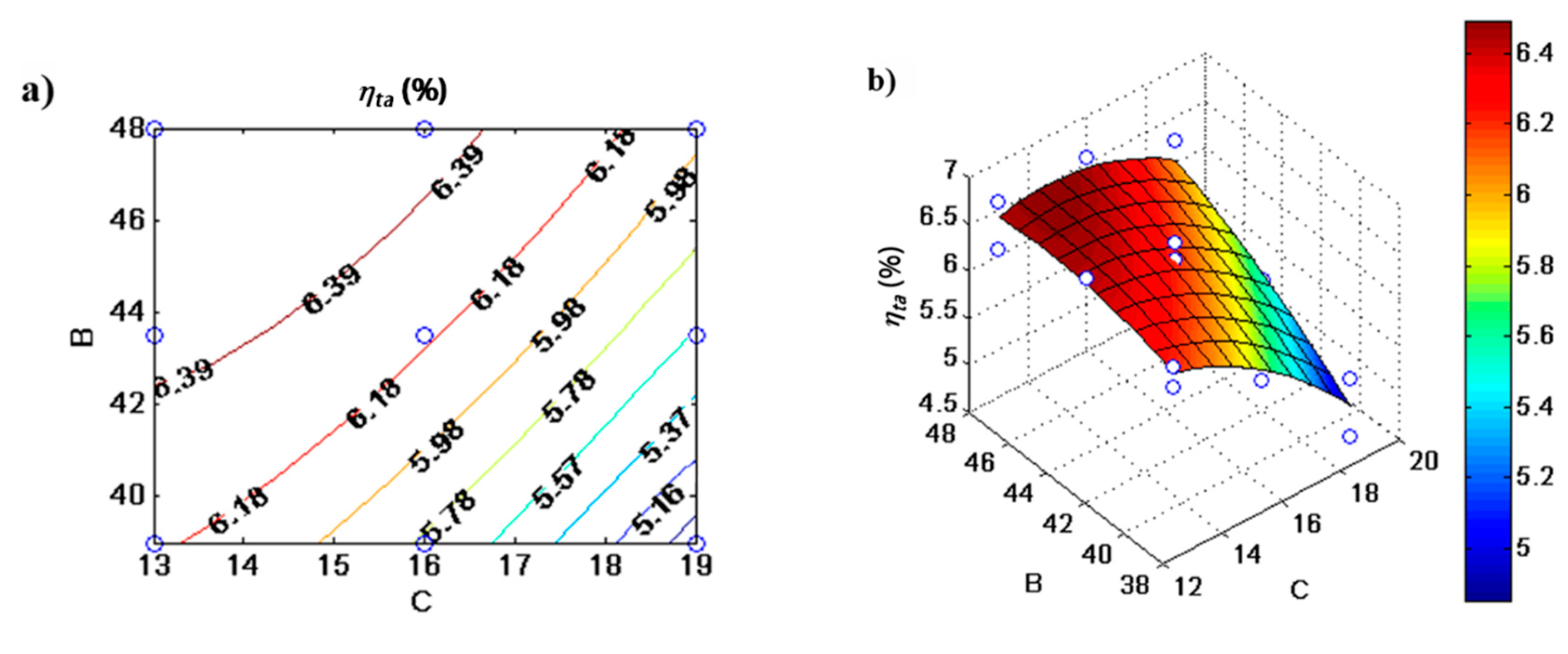
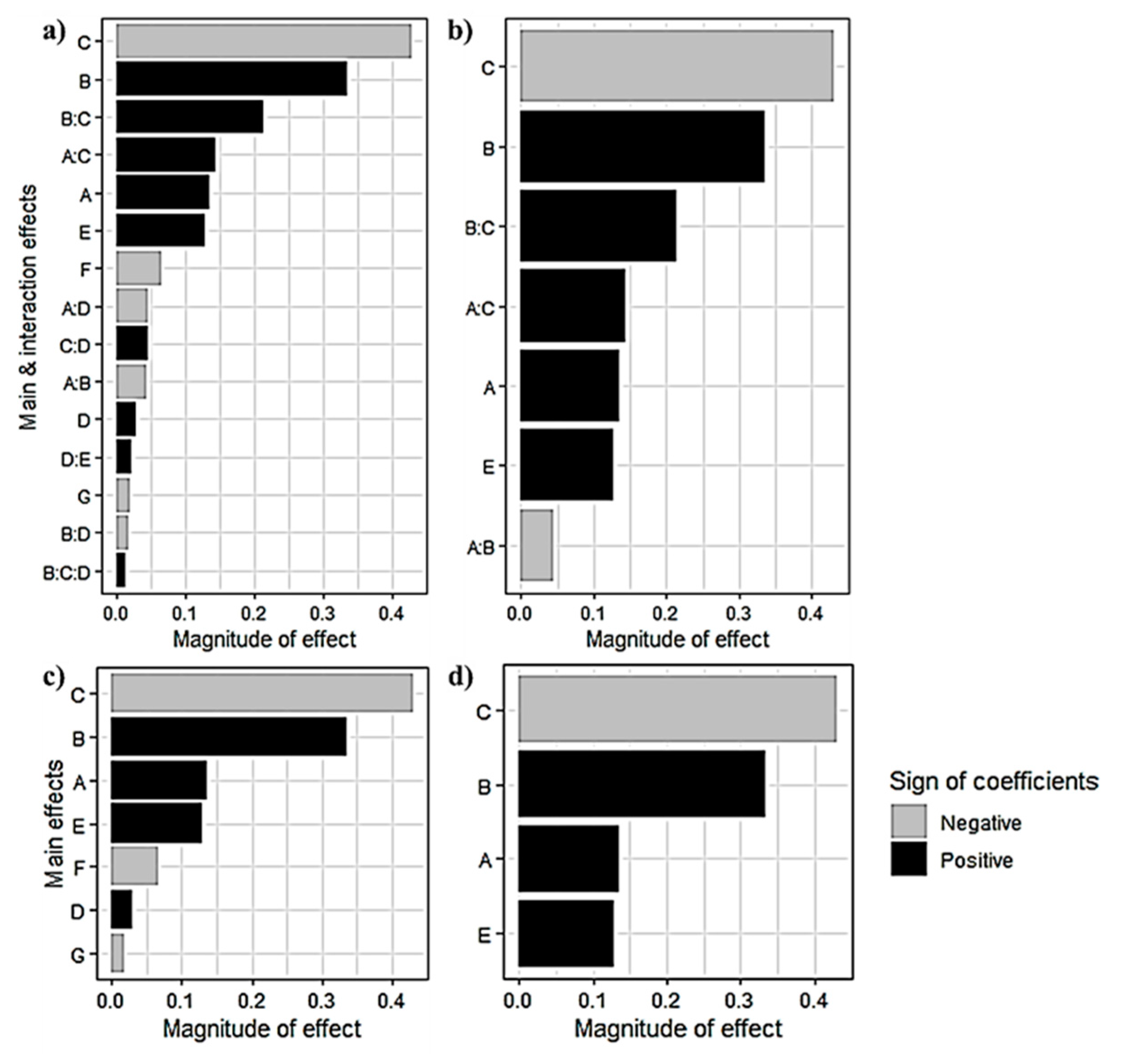
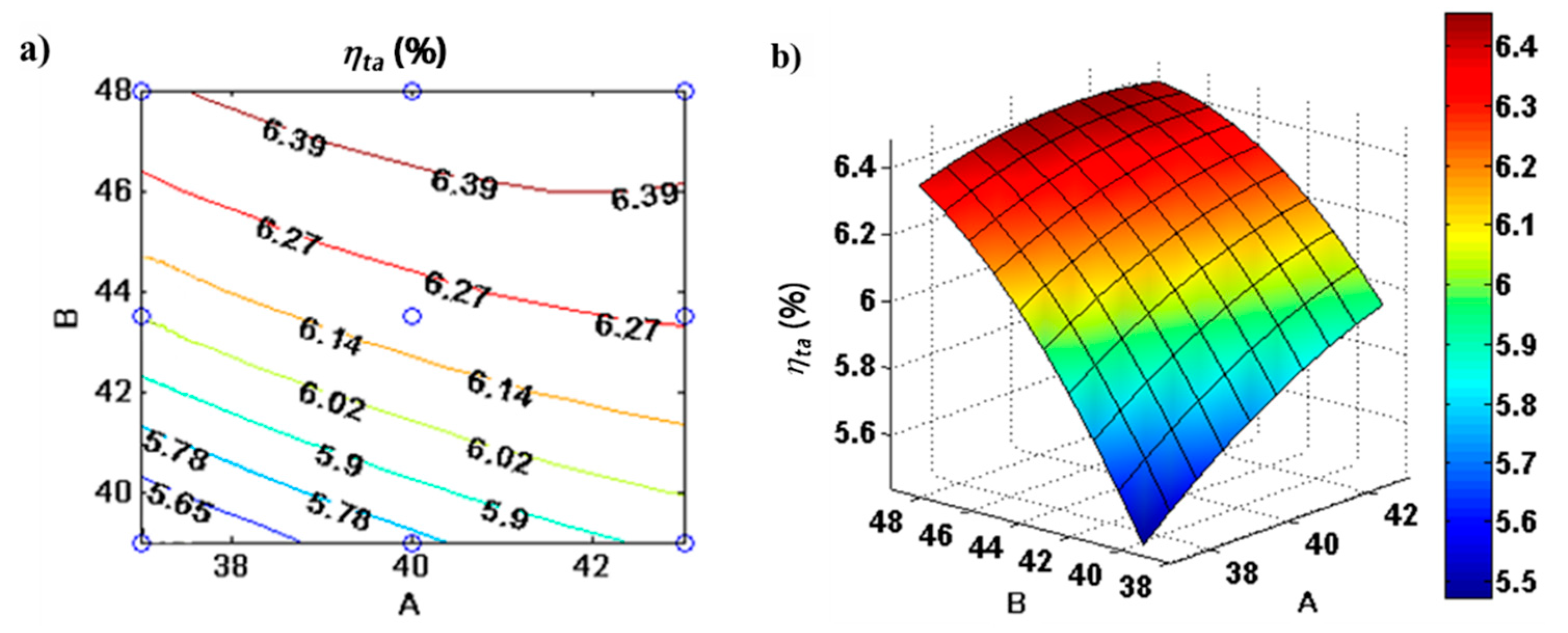
- The compliance inner diameter (B = ) and inertance inner diameter (C = ) are critical parameters for thermoacoustic efficiency. The inertance inner diameter has a reducing effect on the thermoacoustic efficiency, while the compliance inner diameter has an increasing effect;
- The inner diameter of inertance and compliance parameters have significant and positive interaction effects (BC);
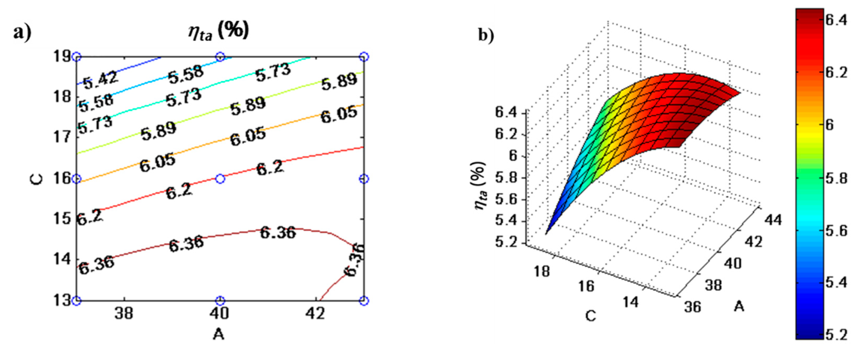
- The operating frequency (A = ) has a positive and relatively smaller impact than factors B and C on thermoacoustic efficiency;
- The operating frequency and inertance inner diameter parameters have positive and mild interaction effects (AC);
- The lengths of the inertance (D = ), the compliance (E = ), the thermal buffer tube (G = G = ), and the hot heat exchanger (F = ) have a negligible effect on thermoacoustic efficiency;
- The operating frequency and compliance inner diameter parameters have negligible interaction effects (AB). Similarly, all the other interactions are negligible.
4. Results
4.1. Response Surface Methodology (RSM)—Faced Centered Design (FCD)
4.2. Model Statistics
4.3. Parametric Analysis
5. Discussion and Conclusions
Author Contributions
Funding
Conflicts of Interest
References
- U.S. Department of Energy Energy efficiency & Renewable Energy. Available online: https://www.fueleconomy.gov/feg/atv.shtml (accessed on 11 October 2019).
- Kölsch, B.; Radulovic, J. Utilisation of diesel engine waste heat by Organic Rankine Cycle. Appl. Therm. Eng. 2015, 78, 437–448. [Google Scholar] [CrossRef] [Green Version]
- Sahoo, D.; Kotrba, A.; Steiner, T.; Swift, G. Waste Heat Recovery for Light-Duty Truck Application Using ThermoAcoustic Converter Technology. SAE Int. J. Engines 2017, 10, 196–202. [Google Scholar] [CrossRef]
- Kim, T.Y.; Kwak, J.; Kim, B. Energy harvesting performance of hexagonal shaped thermoelectric generator for passenger vehicle applications: An experimental approach. Energy Convers. Manag. 2018, 160, 14–21. [Google Scholar] [CrossRef]
- Fernández-Yáñez, P.; Armas, O.; Kiwan, R.; Stefanopoulou, A.G.; Boehman, A.L. A thermoelectric generator in exhaust systems of spark-ignition and compression-ignition engines. A comparison with an electric turbo-generator. Appl. Energy 2018, 229, 80–87. [Google Scholar] [CrossRef]
- Iniesta, C.; Olazagoitia, J.L.; Vinolas, J.; Aranceta, J. Review of travelling-wave thermoacoustic electric-generator technology. Proc. Inst. Mech. Eng. Part A J. Power Energy 2018, 232, 940–957. [Google Scholar] [CrossRef]
- Karlsson, M.; Åbom, M.; Lalit, M.; Glav, R. A Note on the Applicability of Thermo-Acoustic Engines for Automotive Waste Heat Recovery. SAE Int. J. Mater. Manuf. 2016, 9, 286–293. [Google Scholar] [CrossRef]
- Swift, G.W. Thermoacoustics: A Unifying Perspective for Some Engines and Refrigerators, 2nd ed.; ASA Press/Springer: Cham, Switzerland, 2017; ISBN 978-3-319-66932-8. [Google Scholar]
- Ward, B.; Clark, J.; Swift, G. Design Environment for Low-Amplitude Thermoacoustic Energy Conversion DeltaEC Version 6.4b2; Users Guide; Los Alamos National Laboratory: Los Alamos, NM, USA, 2016.
- Saechan, P.; Jaworski, A.J. Numerical studies of co-axial travelling-wave thermoacoustic cooler powered by standing-wave thermoacoustic engine. Renew. Energy 2019, 139, 600–610. [Google Scholar] [CrossRef]
- Backhaus, S.; Swift, G.W. A thermoacoustic-Stirling heat engine: Detailed study. J. Acoust. Soc. Am. 2000, 107, 3148–3166. [Google Scholar] [CrossRef] [PubMed] [Green Version]
- Petach, M.; Tward, E.; Backhaus, S. Design and Testing of A Thermal to Electric Power Converter Based On Thermoacoustic Technology. In Proceedings of the 2nd International Energy Conversion Engineering Conference, American Institute of Aeronautics and Astronauti, Providence, RI, USA, 16–19 August 2004. [Google Scholar]
- Yang, P.; Liu, Y.-W.; Zhong, G.-Y. Prediction and parametric analysis of acoustic streaming in a thermoacoustic Stirling heat engine with a jet pump using response surface methodology. Appl. Therm. Eng. 2016, 103, 1004–1013. [Google Scholar] [CrossRef]
- Hariharan, N.M.; Sivashanmugam, P.; Kasthurirengan, S. Optimization of thermoacoustic refrigerator using response surface methodology. J. Hydrodyn. 2013, 25, 72–82. [Google Scholar] [CrossRef]
- Babu, K.A.; Sherjin, P. Experimental investigations of the performance of a thermoacoustic refrigerator based on the Taguchi method. J. Mech. Sci. Technol. 2018, 32, 929–935. [Google Scholar] [CrossRef]
- Desai, A.B.; Desai, K.P.; Naik, H.B.; Atrey, M.D. Optimization of thermoacoustic engine driven thermoacoustic refrigerator using response surface methodology. IOP Conf. Ser. Mater. Sci. Eng. 2017, 171, 012132. [Google Scholar] [CrossRef]
- Hariharan, N.M.; Sivashanmugam, P.; Kasthurirengan, S. Optimization of thermoacoustic primemover using response surface methodology. HVAC R Res. 2012, 18, 890–903. [Google Scholar]
- Yang, P.; Chen, H.; Liu, Y.W. Application of response surface methodology and desirability approach to investigate and optimize the jet pump in a thermoacoustic Stirling heat engine. Appl. Therm. Eng. 2017, 127, 1005–1014. [Google Scholar] [CrossRef]
- Box, G.; Hunter, J.S.; Hunter, W. Statistics Experimenters; Wiley: New York, NY, USA, 2009; pp. 1–655. [Google Scholar]
- Ihaka, R.; Gentleman, R. R: A Language for Data Analysis and Graphics. J. Comput. Graph. Stat. 1996, 5, 299–314. [Google Scholar]
- Dunn, K.G. Process. Improvement Using Data; McMaster University: Hamilton, ON, Canada, 2010. [Google Scholar]
- Andersson, Ö. Experiment! John Wiley & Sons: New York, NY, USA, 2012; ISBN 9780470688267. [Google Scholar]


| DeltaEC Segment Configuration | Virtual Value |
|---|---|
| BEGIN Operating Conditions | |
| Working gas | Air |
| Mean pressure (pm) | 100 kPa |
| Resonance frequency (f) | 40 Hz |
| Initial temperature of the gas () | 328 K |
| Initial value of pressure amplitude () | 5 kPa |
| Core Branch | |
| Main Cooler (CHX) | |
| Length () | 0.014 m |
| Porosity () | 60% |
| Heat output () | 6 W |
| Regenerator (REG) | |
| Length () | 0.013 m |
| Porosity () | 92% |
| Hydraulic radius () | 0.0002 m |
| Heater (HHX) | |
| Length () | 0.029 m |
| Porosity () | 60% |
| Heat input () | 8 W |
| Thermal buffer tube (TBT) | |
| Length () | 0.101 m |
| Inner diameter () | 0.018 m |
| Secondary Cooler (SCHX) | |
| Length () | 0.01 m |
| Porosity () | 70% |
| Heat output () | 1.9 W |
| Feedback Branch | |
| Compliance (DUCT) | |
| Inner diameter () | 0.0435 m |
| Length () | 0.126 m |
| Inertance (DUCT) | |
| Inner diameter () | 0.016 m |
| Length () | 0.187 m |
| Power Extraction Branch | |
| Mechanical Resonator (IESPEAKER) | |
| Length () | 0.145 m |
| Piston area () | 0.0013 m2 |
| Piston weight () | 0.01 kg |
| Inner diameter () | 0.04 m |
| Mechanical resistance (Rm) | 0.06 N·s m−1 |
| Location & Measurement | Virtual Result |
|---|---|
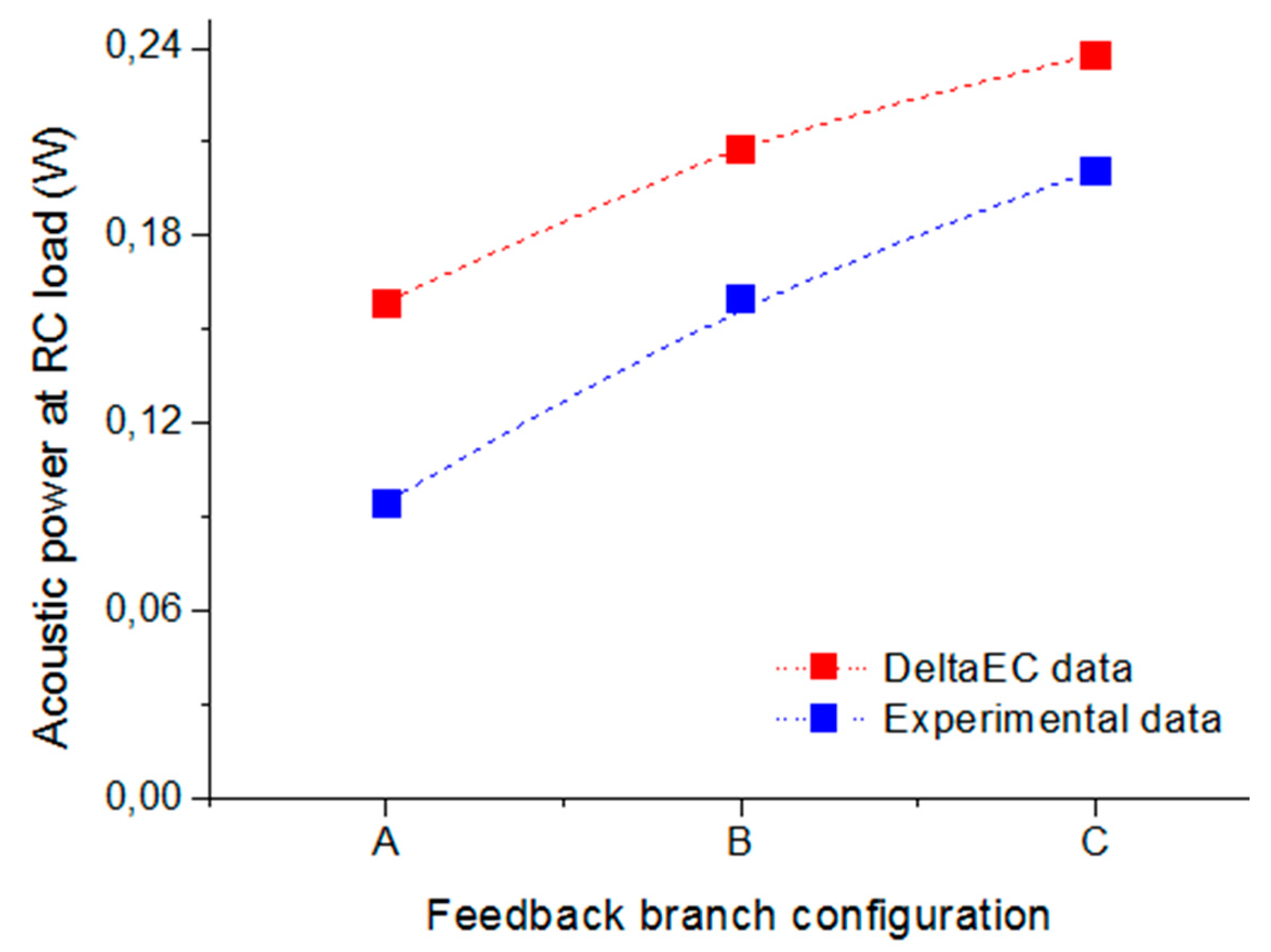
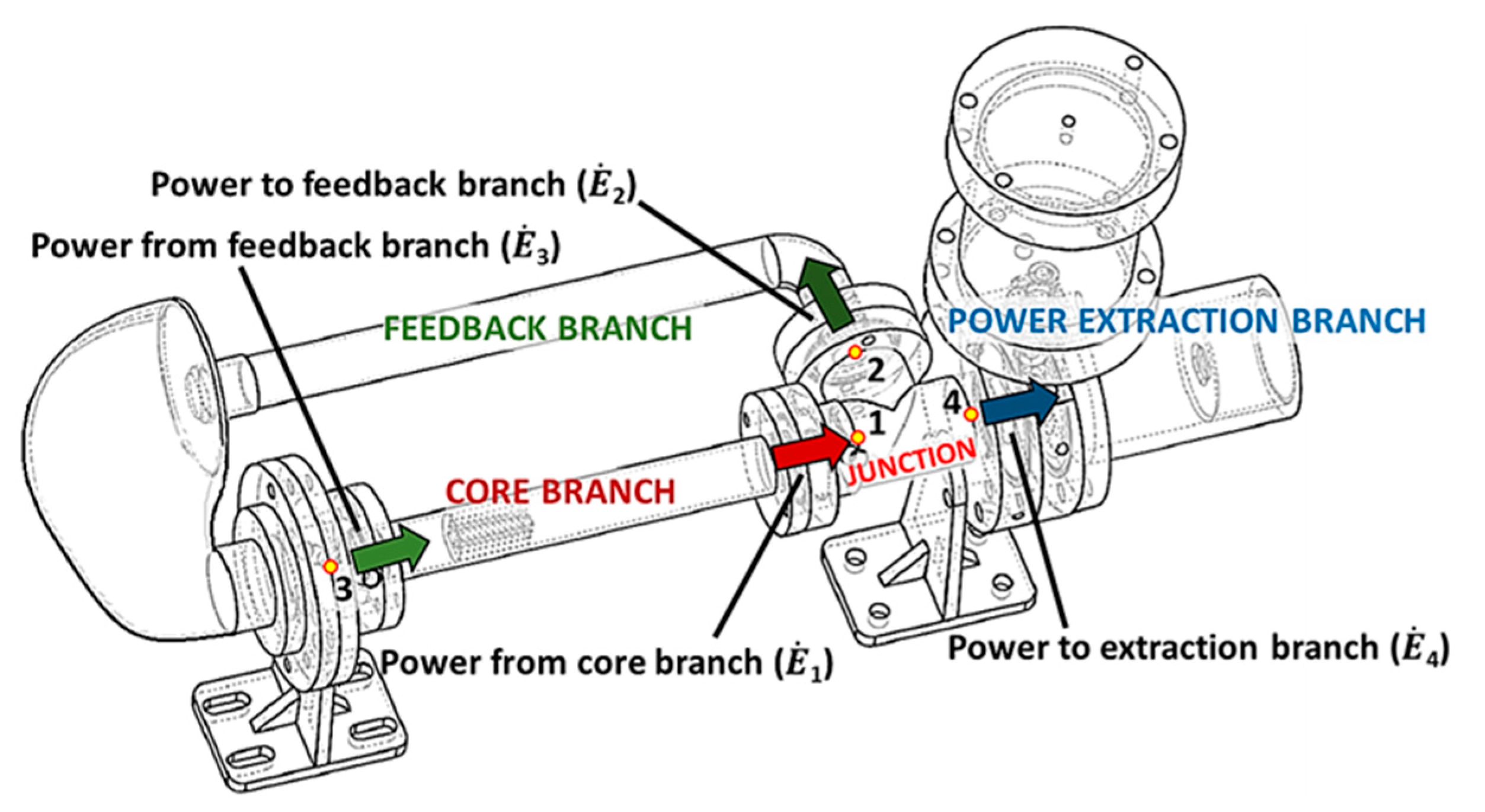
| (1) Acoustic power from core branch | 1.350 W |
| (2) Acoustic power to feedback branch | 0.855 W |
| (3) Acoustic power from feedback branch/to core branch | 0.782 W |
| (4) Acoustic power to power extraction branch | 0.496 W |
| Acoustic power at RC load | 0.238 W |
| Acoustic power rise through core branch | 0.568 W |
| Acoustic power drop through feedback branch | 0.073 W |
| Thermoacoustic efficiency () | 6.199% |
| Factor | Low Level (−1) | High Level (+1) |
|---|---|---|
| Compliance Inner diameter () | 39 mm | 48 mm |
| Compliance Length () | 0.121 m | 0.131 m |
| Inertance Inner diameter () | 13 mm | 19 mm |
| Inertance Length () | 0.182 m | 0.192 m |
| TBT Length () | 0.09 m | 0.112 m |
| Heater Length () | 0.026 m | 0.032 m |
| Resonance Frequency (f) | 37 Hz | 43 Hz |
| Simulation | A | B | C | D | E | F | G | |
|---|---|---|---|---|---|---|---|---|
| 1 | −1 | −1 | −1 | −1 | −1 | −1 | −1 | 6.0072 |
| 2 | +1 | −1 | −1 | −1 | +1 | +1 | +1 | 6.2118 |
| 3 | −1 | +1 | −1 | −1 | +1 | +1 | −1 | 6.4742 |
| 4 | +1 | +1 | −1 | −1 | −1 | −1 | +1 | 6.3441 |
| 5 | −1 | −1 | +1 | −1 | +1 | −1 | +1 | 4.5394 |
| 6 | +1 | −1 | +1 | −1 | −1 | +1 | −1 | 4.9740 |
| 7 | −1 | +1 | +1 | −1 | −1 | +1 | +1 | 5.3908 |
| 8 | +1 | +1 | +1 | −1 | +1 | −1 | −1 | 6.3343 |
| 9 | −1 | −1 | −1 | +1 | −1 | +1 | +1 | 5.9103 |
| 10 | +1 | −1 | −1 | +1 | +1 | −1 | −1 | 6.3628 |
| 11 | −1 | +1 | −1 | +1 | +1 | −1 | +1 | 6.6115 |
| 12 | +1 | +1 | −1 | +1 | −1 | +1 | −1 | 6.0218 |
| 13 | −1 | −1 | +1 | +1 | +1 | +1 | −1 | 4.7358 |
| 14 | +1 | −1 | +1 | +1 | −1 | −1 | +1 | 5.0878 |
| 15 | −1 | +1 | +1 | +1 | −1 | −1 | −1 | 5.7468 |
| 16 | +1 | +1 | +1 | +1 | +1 | +1 | +1 | 6.2608 |
| Simulation | A | B | C | xA | xB | xC | TA-Efficiency | TA-Efficiency |
|---|---|---|---|---|---|---|---|---|
| 0 | 40 | 43.5 | 16 | 0 | 0 | 0 | 6.199 | 6.204 |
| 1 | 37 | 39 | 13 | −1 | −1 | −1 | 6.061 | 6.029 |
| 2 | 43 | 39 | 13 | +1 | −1 | −1 | 6.274 | 6.284 |
| 3 | 37 | 48 | 13 | −1 | +1 | −1 | 6.592 | 6.616 |
| 4 | 43 | 48 | 13 | +1 | +1 | −1 | 6.069 | 6.137 |
| 5 | 37 | 39 | 19 | −1 | −1 | +1 | 4.534 | 4.469 |
| 6 | 43 | 39 | 19 | +1 | −1 | +1 | 5.158 | 5.136 |
| 7 | 37 | 48 | 19 | −1 | +1 | +1 | 5.693 | 5.685 |
| 8 | 43 | 48 | 19 | +1 | +1 | +1 | 6.235 | 6.269 |
| FC+ | 40 | 43.5 | 19 | 0 | 0 | +1 | 5.486 | 5.546 |
| FB− | 40 | 39 | 16 | 0 | −1 | 0 | 5.641 | 5.749 |
| FA+ | 43 | 43.5 | 16 | +1 | 0 | 0 | 6.372 | 6.281 |
| FC− | 40 | 43.5 | 13 | 0 | 0 | −1 | 6.494 | 6.423 |
| FB+ | 40 | 48 | 16 | 0 | +1 | 0 | 6.566 | 6.447 |
| FA− | 37 | 43.5 | 16 | −1 | 0 | 0 | 5.944 | 6.024 |
| Coefficients | SS | Df | MS | F-Value | p-Value |
|---|---|---|---|---|---|
| FCD Model | 4.4901 | 9 | 0.4989 | 26.0045 | 0.00039 |
| A (f) | 0.3214 | 1 | 0.3214 | 16.7396 | 0.00346 |
| B | 1.3072 | 1 | 1.3072 | 68.0833 | 0.000007 |
| C | 2.0495 | 1 | 2.0495 | 106.7448 | 0.000002 |
| AB | 0.1345 | 1 | 0.1345 | 7.0052 | 0.01785 |
| AC | 0.2831 | 1 | 0.2831 | 14.7448 | 0.00086 |
| BC | 0.4560 | 1 | 0.4560 | 23.75 | 0.00018 |
| Residual | 0.1151 | 6 | 0.0192 | - | - |
| Lack of fit | 0.1151 | 5 | 0.0230 | - | - |
| Total | 4.6052 | 15 | - | - | - |
© 2019 by the authors. Licensee MDPI, Basel, Switzerland. This article is an open access article distributed under the terms and conditions of the Creative Commons Attribution (CC BY) license (http://creativecommons.org/licenses/by/4.0/).
Share and Cite
Iniesta, C.; Olazagoitia, J.L.; Vinolas, J.; Gros, J. Energy and Efficiency Evaluation of Feedback Branch Design in Thermoacoustic Stirling-Like Engines. Energies 2019, 12, 3867. https://doi.org/10.3390/en12203867
Iniesta C, Olazagoitia JL, Vinolas J, Gros J. Energy and Efficiency Evaluation of Feedback Branch Design in Thermoacoustic Stirling-Like Engines. Energies. 2019; 12(20):3867. https://doi.org/10.3390/en12203867
Chicago/Turabian StyleIniesta, Carmen, José Luis Olazagoitia, Jordi Vinolas, and Jaime Gros. 2019. "Energy and Efficiency Evaluation of Feedback Branch Design in Thermoacoustic Stirling-Like Engines" Energies 12, no. 20: 3867. https://doi.org/10.3390/en12203867
APA StyleIniesta, C., Olazagoitia, J. L., Vinolas, J., & Gros, J. (2019). Energy and Efficiency Evaluation of Feedback Branch Design in Thermoacoustic Stirling-Like Engines. Energies, 12(20), 3867. https://doi.org/10.3390/en12203867