Three-Dimensional Numerical Simulation of Geothermal Field of Buried Pipe Group Coupled with Heat and Permeable Groundwater

Abstract

The flow of groundwater and the interaction of buried pipe groups will affect the heat transfer efficiency and the distribution of the ground temperature field, thus affecting the design and operation of ground source heat pumps. Three-dimensional numerical simulation is an effective method to study the buried pipe heat exchanger and ground temperature distribution. According to the heat transfer control equation of non-isothermal pipe flow and porous media, combined with the influence of permeable groundwater and tube group, a heat-transfer coupled heat transfer model of the buried pipe group was established, and the accuracy of the model was verified by the sandbox test and on-site thermal response test. By processing the layout of the buried pipe in the borehole to reduce the number of meshes and improve the meshing quality, a three-dimensional numerical model of the buried pipe cluster at the site scale was established. Additionally, the ground temperature field under the thermal-osmotic coupling of the buried pipe group during groundwater flow was simulated and the influence of the head difference and hydraulic conductivity on the temperature field around the buried pipe group was calculated and analyzed. The results showed that the research on the influence of the tube group and permeable groundwater on the heat transfer and ground temperature field of a buried pipe simulated by COMSOL software is an advanced method.

1. Introduction

Ground heat exchanger (GHE), which is also called a geothermal heat exchanger, has emerged as a promising and globally accepted way of exploiting shallow geothermal energy. Typically, circulating heat-carrying fluids flow in a U-shaped channel inserted in a vertical borehole and absorb or discharge heat from or to the ground [1]. The performance of ground source heat pump (GSHP) systems, constructed with many GHEs, is determined by ground stratigraphy in which thermal conductivity, groundwater flow, and the initial temperature play an essential role [2,3]. Knowledge of the thermal processes in the ground is not only critical for the optimal design and operation of systems (GSHP) [4,5,6], but is also a prerequisite in evaluating their relevance and the hazards related to the local climatic conditions and geological context [7].

In order to estimate the heat transfer of borehole heat exchangers (BHEs), based on the pioneering work of Ingersoll et al. [4], diverse numerical and analytical methods have been proposed [8]. Plenty of research has focused on the system design, penalty temperature prediction [9], parameter estimation [10,11], quasi-steady heat transfer around a borehole [12], and progress in conventional models for borehole GHEs [13]. The buried depth of BHEs is about 60–300 m, where groundwater exists and its flow benefits the heat transfer and reduces or eliminates the accumulating imbalance effects of heat transfer [14,15,16,17,18,19].

The thermal response test (TRT), designed based on the infinite line source model (ILS), is the most common approach to describe the heat conduction process in homogeneous media with a constant temperature at infinity [20]. Several studies have been conducted to analyze the importance of groundwater on heat transfer in TRTs. Diao et al. [21,22] obtained an analytical solution of two-dimensional temperature response with uniform permeability through a line heat source in the infinite field by means of the Green function analysis. Molina-Giraldo et al. [23] deduced an analytical solution through the use of the moving finite line source model (MFLS) with the consideration of the groundwater flow and axial effects. Wagner et al. [24,25] proposed a parameter estimation method which was sensitive to conduction and advection to calculate the actual Darcy velocity based on MFLS. Aranzabal et al. [26] complemented the standard TRT analysis and estimated the thermal conductivity profile from the borehole temperature profile during the test.

With the wider utilization of GSHPs, the scale of projects is increasing with hundreds, even thousands, of groups of borehole heat exchangers [27]. The heat transfer in the underground heat exchanger groups is coupled and interacts with each other in the actual operation process, so some single hole research conclusions cannot be directly applied [28]. The long-term research models for buried pipe groups mainly include the two-dimensional heat transfer model and three-dimensional heat transfer model. Most researchers have often used two-dimensional models to study the long-term variation of the temperature field in a buried tube region [29,30,31]. Jia constructed 2D and 3D unsteady heat transfer models of vertical U-tube GHEs based on practical projects [32]. Yang et al. established a 3D heat transfer model of a ground heat exchanger that couples thermal conduction with groundwater flow, and pointed out that the heat transfer capacity of staggered arrangement was higher than that of an aligned arrangement, which is made more obvious by the groundwater flow [33].

In summary, the research on the heat transfer model of buried pipes has always been a difficult point in the technology of ground source heat pump systems. The influence of groundwater flow on the heat transfer of buried pipes has been of high concern, and relevant research has made great progress. However, many of the buried pipe models have been simplified, based on the mobile line heat source. The true line heat source can give an exact solution, and the splitting of the flow field and the temperature field cannot obtain a more accurate analytical solution model. It is more practical to establish a physical model that is exactly the same as the shape of the actual buried pipe [34].

There are few studies on the interaction between long-running buried pipe groups, and the impact of groundwater flow on buried pipe groups has rarely been considered. Numerical simulation is very time consuming in solving the formation temperature field of the three-dimensional buried tube group thermal-permeability coupling in the whole year or the whole life cycle, especially in calculating the temperature distribution of all-time nodes and spaces of the large buried tube group.

In the research work of this paper, based on the non-isothermal pipe flow module in the finite-element numerical simulation software COMSOL, the buried pipe was simplified into a three-dimensional curve, and the fluid heat transfer, velocity, and pressure in the buried pipe were solved. A new simplified model of the buried pipe was proposed to improve the efficiency and accuracy of the finite element numerical model calculation. The porous medium heat transfer module and the groundwater flow module were used to solve the heat-transfer coupling heat transfer process in the soil. The influence of the buried pipe group and the thermal transfer coupling on the formation temperature field was studied after one year of operation. The simplified model could accurately solve the temperature response of the formation in the long-term heat transfer process of the buried tube group with limited computational resources.

This paper is mainly composed of the following parts: First, the governing equation of the heat transfer in the formation coupling heat transfer of the buried pipe was given, then the simplified physical model of the buried pipe heat transfer was established. Second, based on the sandbox test data and on-site thermal response test data, the finite element simulation software COMSOL was used to simulate and verify the full-scale three-dimensional buried tube thermal-permeability coupling model, which confirmed the accuracy and practicability of the simplified model. Third, a numerical model of the thermal infiltration coupling of the full-scale buried pipe group was established. When the different hydraulic conductivities were calculated, the temperature field distribution in the formation after one year of system operation was obtained. The effects of different hydraulic conductivity on the formation temperature field were obtained.

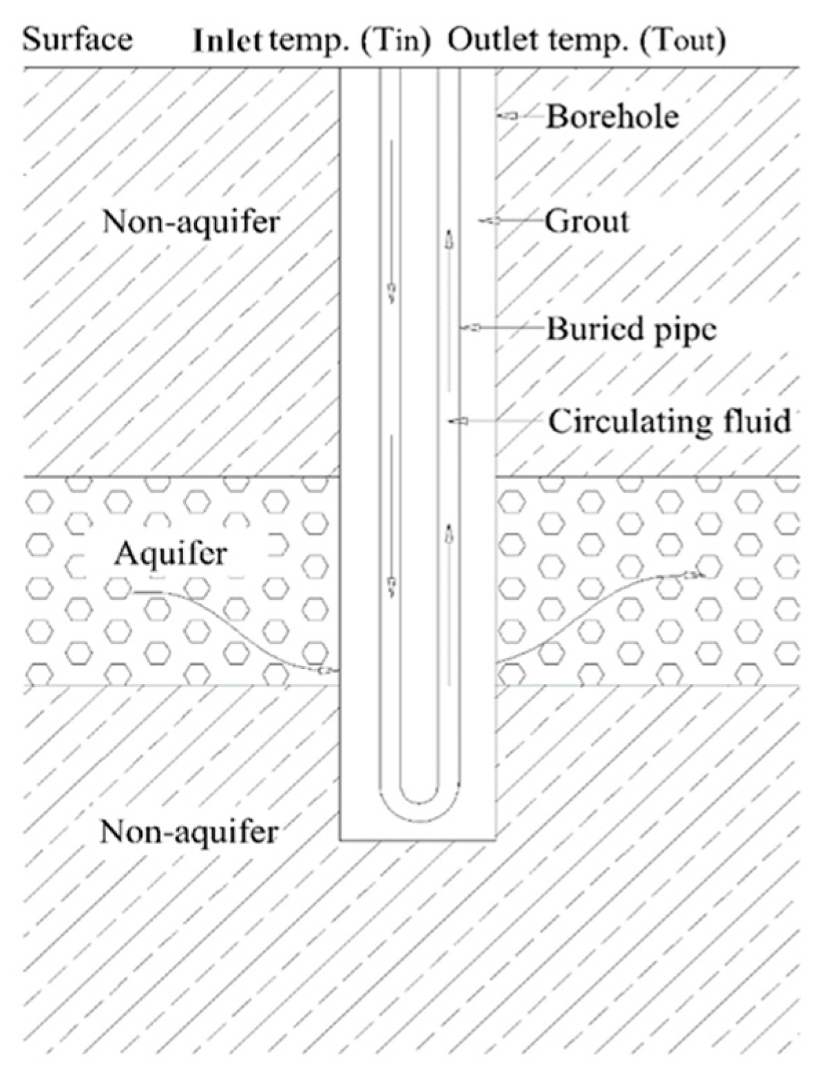
2. Establishment of Heat Transfer Models for A Single Well Buried Pipe Coupled with Flow of Groundwater

The heat exchange process between the buried pipe and the soil can be divided into heat conduction between the circulating fluid in the U-shaped pipe and the pipe wall, heat conduction between the buried pipe wall and the backfill material, and heat conduction between the backfill material and the soil. The non-isothermal pipe flow module based on the finite element numerical simulation software COMSOL Multiphysics 5.3 simulates the heat transfer process of the circulating fluid in the buried pipe; the heat transfer coupling heat transfer process in the soil is simulated by the porous medium heat transfer module and the Darcy permeable module. A schematic diagram of the buried pipe is shown in Figure 1.

2.1. Establishment of Governing Equations for Coupled Model of Buried Pipe with Heat and Groundwater

The control equations of heat transfer between the pipeline and porous formation with Darcy’s fluid are deduced according to the principle of the conservation of energy.

(1)

Energy equation for pipeline flow

It is assumed that the fluid in each section of the pipe is in a fully developed state and is transient-state heat transfer. The velocity, pressure, and temperature at the same section are the same, and change only along the axial direction of the pipe. The circulating fluid in the buried pipe is considered as incompressible flow. The heat balance equation of the fluid in the pipe is as follows:

$$\rho A{C}_p\frac{\partial T}{\partial t}+\rho A{C}_p{\mathrm{u}}_{et}·{\nabla }_{t}T={\nabla }_t·\left(A\lambda {\nabla }_{t}T\right)+\frac{1}{2}{f}_D\frac{\rho A}{2d_h}\left|u\right|u^2+Q_p+Q_{wall}$$

(1)

$$A=\frac{\pi }{4}{d}_i^2$$

(2)

$$f_D=8{[{\left(\frac{8}{R_e}\right)}^{12}+{\left(C_A+C_B\right)}^{-1.5}]}^{\frac{1}{12}}$$

(3)

$$R_e=\frac{\rho \mathrm{u}{d}_i}{\mu }$$

(4)

$$C_A={\left[-2.457\ln ({\left(\frac{7}{R_e}\right)}^{0.9}+0.27\left(\frac{e}{d_i}\right))\right]}^{16}$$

(5)

$$C_B={(\frac{37530}{R_e})}^{16}$$

(6)

$$Q_{wall}={\left(hZ\right)}_{eff}\left(T_{ext}-T\right)$$

(7)

$$Z=\pi d_i$$

(8)

where $\rho$ is the fluid density in the pipe, kg/m³; A is the pipe cross-sectional area, m²; $C_p$ is the isobaric heat capacity of fluid, J/(kg·K); $u_{et}$ is the tangential velocity, m/s; $T$ is the temperature of the fluid, K$; \lambda$ is the thermal conductivity of fluid, W/(m·K);$f_D$ is the friction coefficient;$d_i$ is the pipe inner diameter, m; $\mathrm{u}$ is the mean velocity of fluid, m/s; $Q_p$ is the heat source/sink item in the pipe, W/m (as the pipe in this study does not have an extra heat source, $Q_p$ is zero); $Q_{wall}$ is the heat exchange on the pipe wall, W/m; ${\left(hZ\right)}_{eff}$ is the effective total thermal resistance of the pipe wall, W/(m∙K), which includes the thermal resistance of the pipe and the thermal resistances of the inner and outer pipe wall with the convection layer [35]; h is the heat transfer coefficient, W/(m²∙K); Z is the wetted perimeter of the pipe, m; $T_{ext}$ is the exterior temperature outside pipe, K; and T is the fluid temperature inside the pipe, K [36,37].

(2)

Energy equation for pipeline flow for porous formation

Heat transfer in porous water-bearing formations can be expressed by the following equation:

$$Q_f+Q_{geo}={\left(\rho C_p\right)}_{eq}\frac{\partial T_f}{\partial t}+\rho C_{p}v·\nabla T_f-\nabla ·\left({\lambda }_{eq}\nabla T_f\right)$$

(9)

where $Q_f$ is the heat source/sink item in the formation, W/m; $Q_{geo}$ is the special geothermal heating function (expressed as domain conditions) in the porous media heat transfer interface, W/m. Since there was no extra heat source or sink and special geothermal heating in the ground of this study, the terms of $Q_f$ and $Q_{geo}$ were set as zero; ${\left(\rho C_p\right)}_{eq}$ is the equivalent volumetric specific heat, J/(m³·K); $v$ is the groundwater flow velocity, m/s; $\nabla T_f$ is the incremental temperature of formation, K; and ${\lambda }_{eq}$ is the equivalent thermal conductivity, W/(m·K).

The average value of the thermal parameters of the soil is expressed as a weighting factor, expressed as matrix volume fraction θ. In saturated formation, the pore is occupied by water, while in unsaturated formation, water and air may exist in the pore. Using the volume averaging method, the volumetric specific heat of the heat transfer equation in formation is:

$${\left(\rho C_p\right)}_{eq}={\displaystyle \sum }_i\left({\theta }_i{\rho }_i{C}_{pi}\right)+\left(1-{\displaystyle \sum }_i{\theta }_i\right){\rho }_s{C}_{ps}$$

(10)

where ${\theta }_i$ is the volume ratio of the ith non-solid in the formation$; {\rho }_i$ is the density of the ith non-solid material, kg/m³; $C_{pi}$ is specific heat capacity of the ith non-solid material, J/(kg·K); ${\rho }_s$ is the density of solid, kg/m³; and $C_{ps}$ is the specific heat capacity of the solid, J/(kg·K).

The equivalent thermal conductivity is described as:

$${\lambda }_{eq}={\displaystyle \sum }_i{\theta }_i{\lambda }_i+\left(1-{\displaystyle \sum }_i{\theta }_i\right){\lambda }_{\mathrm{s}}$$

(11)

where ${\lambda }_i$ is the thermal conductivity of the ith non-solid material, W/(m·K) and ${\lambda }_s$ is the thermal conductivity of solid, W/(m·K).

(3)

The permeable equation of fluid flowing in porous formation

According to the universal conservation principle proposed, the mass conservation equation describing the underground hot water system can be written as follows:

$$\frac{\partial }{\partial t}\left({\rho }_w\mathsf{\phi }\right)+\nabla ·\left({\rho }_{w}v\right)={\rho }_q{q}_s$$

(12)

where t is the time, s; ${\rho }_w$ is the groundwater density, kg/m³;$\mathsf{\phi }$ is the effective porosity, dimensionless; $v$ is the permeable velocity of groundwater, m/s; ${\rho }_q$ is the density of source sink source, kg/m³; and $q_s$ is the source sink term, 1/s.

Darcy’s law expresses different permeable flow as follows:

$$v=-\frac{k\rho g}{\mu }\nabla H$$

(13)

where $k$ is permeability, m²; $g$ is the gravity acceleration, m/s²; $\mu$ is the dynamic viscosity of groundwater, Pa∙s; and $H$ is the hydraulic head, m.

2.2. Initial Condition and Boundary Conditions

2.2.1. Initial Condition

Before the fluid flows into the pipe, the temperature of the pipe and formation is distributed as the initial formation temperature.

$${T|}_{t=0}={T_f|}_{t=0}=T_{ei}$$

(14)

where $T_{ei}$ is the initial formation temperature, °C.

2.2.2. Boundary Conditions

The temperature of fluid in the pipe at the surface is the inlet temperature:

$${T|}_{z=0}=T_{in}$$

(15)

where $T_{in}$ is inlet temperature of fluid in the pipe, °C.

The formation temperature does not change along the horizontal at infinity, i.e.:

$${\frac{d{T}_f}{dx}|}_{x\to \infty }={\frac{d{T}_f}{dy}|}_{y\to \infty }=0$$

(16)

The formation at the surface and the bottom is adiabatic, then,

$$-{\lambda }_{eq}{\frac{d{T}_f}{dz}|}_{z=0}=-{\lambda }_{eq}{\frac{d{T}_f}{dz}|}_{z=L}=0$$

(17)

where,$L$ is the depth of the formation, m.

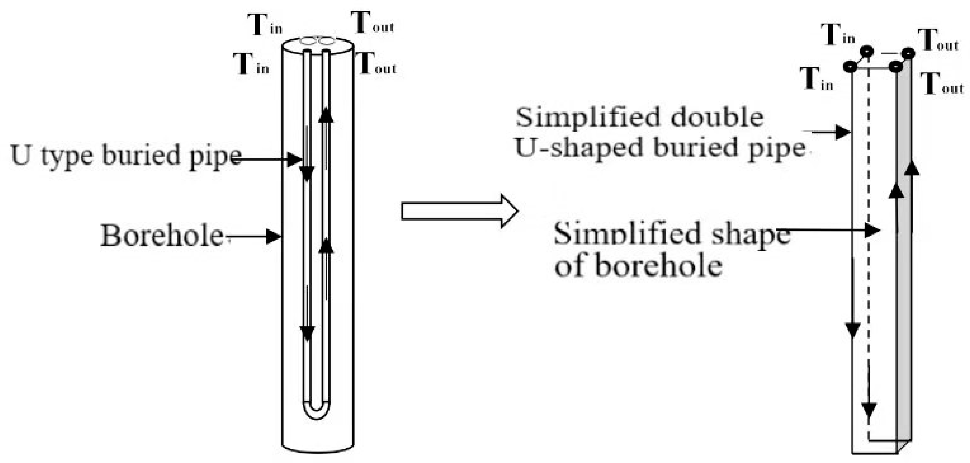
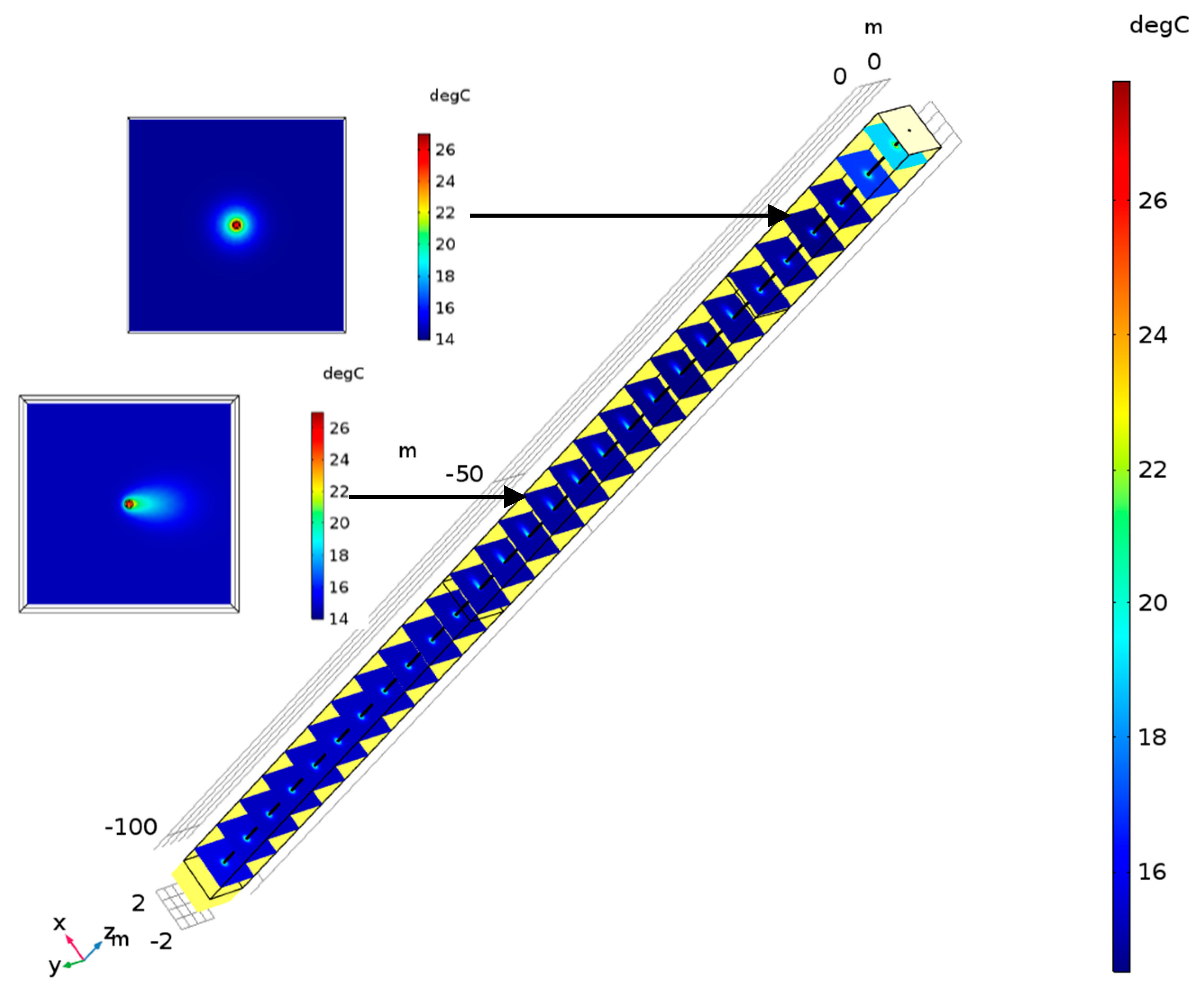
2.3. Simplification of the Buried Pipe Model

As the length of the buried pipe often exceeds 100 m, and the radial dimension of the buried pipe is within 36 mm, conducting the length of the buried pipe is much larger than the radial dimension, which is not conducive to the division of the buried pipe mesh and the network is in poor quality. The non-isothermal pipe flow module in COMSOL can simplify the problem of pipe flow with a finite diameter to the problem of fluid flow velocity, temperature, and pressure in the calculation curve, which is beneficial to mesh segmentation and greatly improves the efficiency of the pipe fluid simulation calculation.

The drilling hole was simplified into a very long cuboid with a long length of borehole depth and a square end with sides equal to the borehole diameter. The buried pipe was simplified as curves arranged along the four long sides of the cuboid. The buried pipe was modeled and the model was simplified as shown in Figure 2.

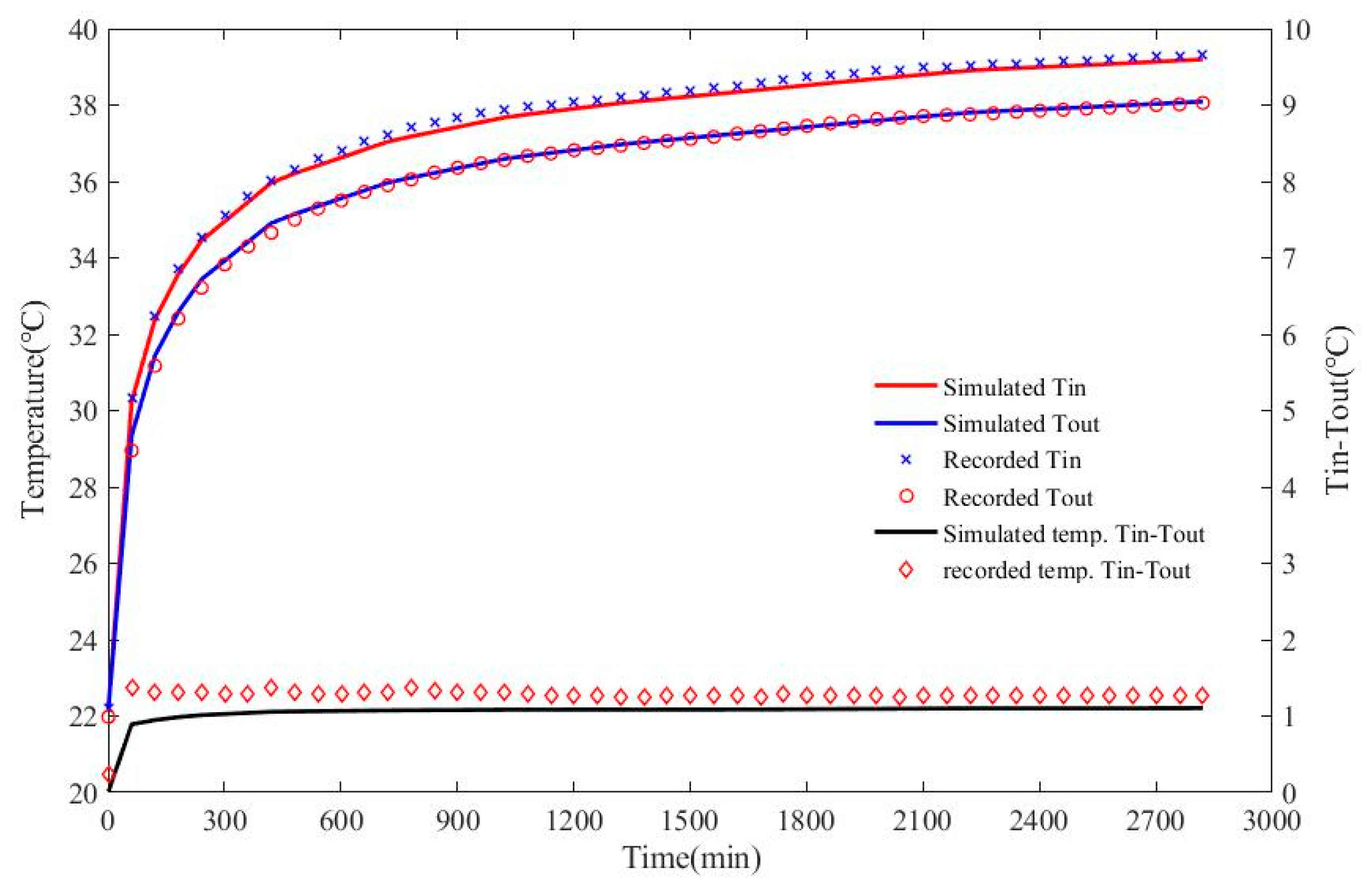
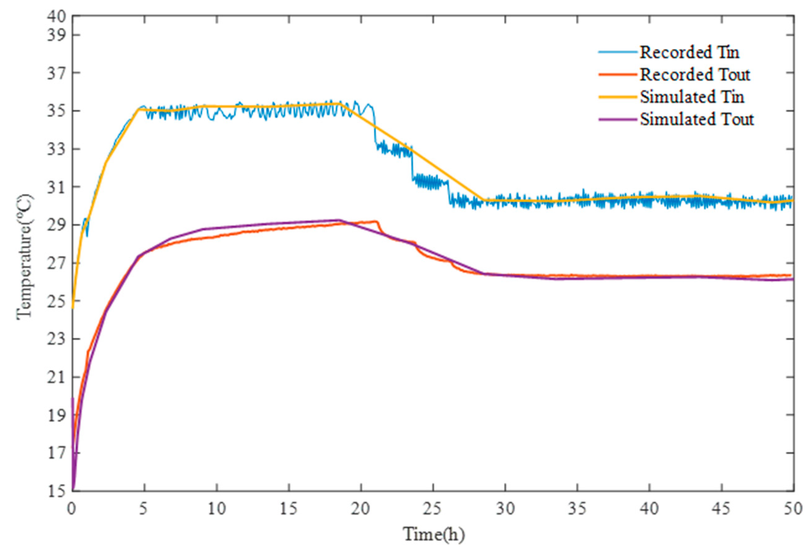
2.4. Simplified Model Verification

Based on the heat-induced coupled heat transfer control equation in Section 2.1 and Section 2.3, a three-dimensional numerical model of a full-scale buried tube thermal-permeability coupling was established by using the non-isothermal pipe flow module of COMSOL, the porous medium heat transfer module, and Darcy permeable module. The non-isothermal pipe flow module simulates the heat transfer of the circulating fluid in the buried pipe, and the porous medium and the groundwater permeable module simulate the heat-induced coupled heat transfer in the soil.

In order to verify the accuracy of the model, this paper first used the sandbox test data to verify the small size model. Then, a full-scale model verification was performed based on the on-site thermal test. The boundary conditions around the soil were set to adiabatic boundaries, the temperature values were the same as the initial values of the formation, and the top surface temperature of the model was set to 25 °C. The inlet of the buried pipe was set to a known flow velocity boundary, and the outlet was set to a constant pressure boundary. The following assumptions were made in the model: (1) The temperature around the tube is equal; (2) The velocity direction of the fluid in the buried tube is along the tube axis; and (3) the heat transfer in the tube wall is quasi-static.

2.4.1. Sandbox Test Verification

The sandbox test presented by Beier was used to verify the model above. The size of the sand box was 18.3 m × 1.8 m × 1.8 m, an aluminum pipe was regarded as the borehole wall where the inner diameter was 12.6 cm and the thickness was 0.2 cm. The length, inner radius, and outer radius of the U-tube pipe were 18.3 m, 2.733 cm, and 3.340 cm, respectively. The volumetric flow rate was 0.197 L/s. The thermal conductivities of the soil and grout were 2.82 W/(m·K) and 0.73 W/(m·K), respectively, and the sand porosity was 0.89, the specific heat capacity was 1900 J/(kg·K), and the density was 1200 kg/m³ [38]. Based on the simplified buried pipe model in Section 2.2 and the sandbox size and test conditions, a numerical model was established. The numerical simulation of the sandbox test was carried out by using the non-isothermal pipe flow module, porous medium heat transfer module, and groundwater permeable module in COMSOL. The results are shown in Figure 3. The solid blue line is the simulated value of the outlet temperature, and the red hollow dot is the recorded value of the outlet temperature. It can be seen that the two agreed well, and the measured outlet temperature value differed from the simulated outlet temperature by a maximum of 0.2 °C, confirming the accuracy of the simplified model.

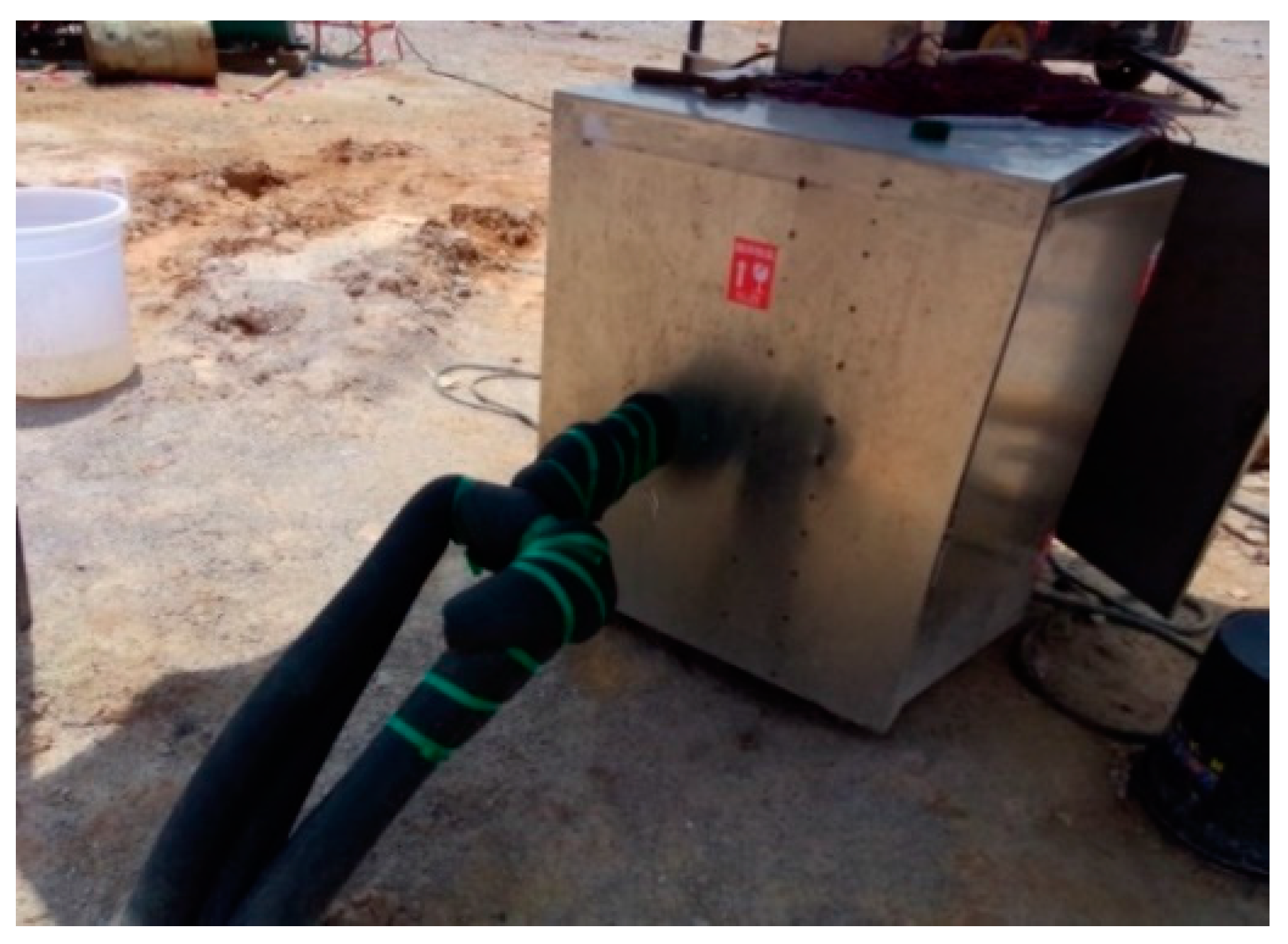
2.4.2. On-Site Thermal Response Test Verification

In order to further verify the simplified model to simulate the mesh length quality, calculation efficiency, and accuracy of the buried pipe with a large aspect ratio, the on-site thermal response test was simulated and verified. The outdoor test address was located in Baimiao Village, Tongzhou District, Beijing, with a total of nine drill holes. The initial temperature of the formation was first measured and then an on-site thermal response test was carried out. Twelve temperature measuring points were arranged in each of the #1 hole and the #2 hole, and the depth and temperature of the temperature measuring point in the hole were as shown in

Table 1. Initial formation temperature.

Depth (m)	−5	−10	−15	−20	−30	−40
#1 temperature (°C)	17.11	14.25	14.81	14.87	14.50	14.80
#2 temperature (°C)	17.13	14.63	14.81	14.88	14.44	14.81
Depth (m)	−50	−60	−70	−80	−90	−100
#1 temperature (°C)	14.87	15.01	15.24	15.37	15.24	15.87
#2 temperature (°C)	14.88	15.06	15.25	15.38	15.19	15.88

.

Then, the on-site thermal response test was carried out on the #1 hole and the #2 hole, respectively. The #1 hole was used for the constant temperature condition. The inlet and outlet temperature data of the buried pipe was used to measure the thermal property parameters of the formation; the #2 hole was used for the constant power condition and buried. The tube inlet and outlet temperature data were used to validate the simplified buried tube model. To obtain a more accuracy thermal conductivity, two situations where the inlet temperature was 30 °C and 35 °C were adopted during the test. The on-site thermal response test is shown in Figure 4.

Based on the on-site thermal response test data, a numerical model of the full-scale three-dimensional thermal response test was established based on the simplified buried pipe physical model. The parameters in the model were the same as the on-site thermal response test parameters, as shown in

Table 2. Thermal response test and formation thermal property parameters.

Name	Unit	Number
The depth of the hole	m	102
The depth of ground pipe	m	100
The diameter of Drilling	mm	150
The outer diameter of buried tube	mm	32
The inner diameter of buried tube	mm	26
U-tube spacing	mm	100
The flow rate of circulating fluid	m³/h	1.1
Effective thermal conductivity	W/(m·K)	1.86
Formation specific heat capacity	kJ/(kg·K)	2.80
U-tube thermal conductivity	W/(m·K)	0.44
The roughness of wall surface	mm	0.0015
The conductivity of backfill material thermal	W/(m·K)	2.3
The capacity of backfill material specific heat capacity	kJ/(kg·K)	0.84

.

The bottom plane of the borehole was divided according to the free-distributed triangle mesh, and then the borehole mesh was generated by sweeping the bottom surface of the source’s surface along the drill depth direction. The total number of mesh was 321,157, the minimum unit mass was 0.28, the average unit mass was 0.83, the minimum unit size was 0.05 m, the maximum unit size was 0.44 m, and the time step was 5 min. The thermal response test simulation results are shown in Figure 5.

We compared the measured outlet temperature value of the buried pipe with the outlet temperature calculated by the numerical model, as shown in Figure 6. The solid line in red in the figure is the simulated outlet temperature, and the purple solid line is the recorded outlet temperature in the thermal response experiment. The outlet temperature calculated by the numerical model was basically consistent with the outlet temperature recorded in the field, and the accuracy of the established three-dimensional numerical model of the buried tube thermal-osmotic coupling was verified. The simplified buried pipe physical model greatly reduced the total number of meshes on the basis of ensuring the quality of meshing. In order to establish a thermal-osmotic coupling model of the buried pipe group in accordance with the actual size under limited computing resources, the foundation was laid.

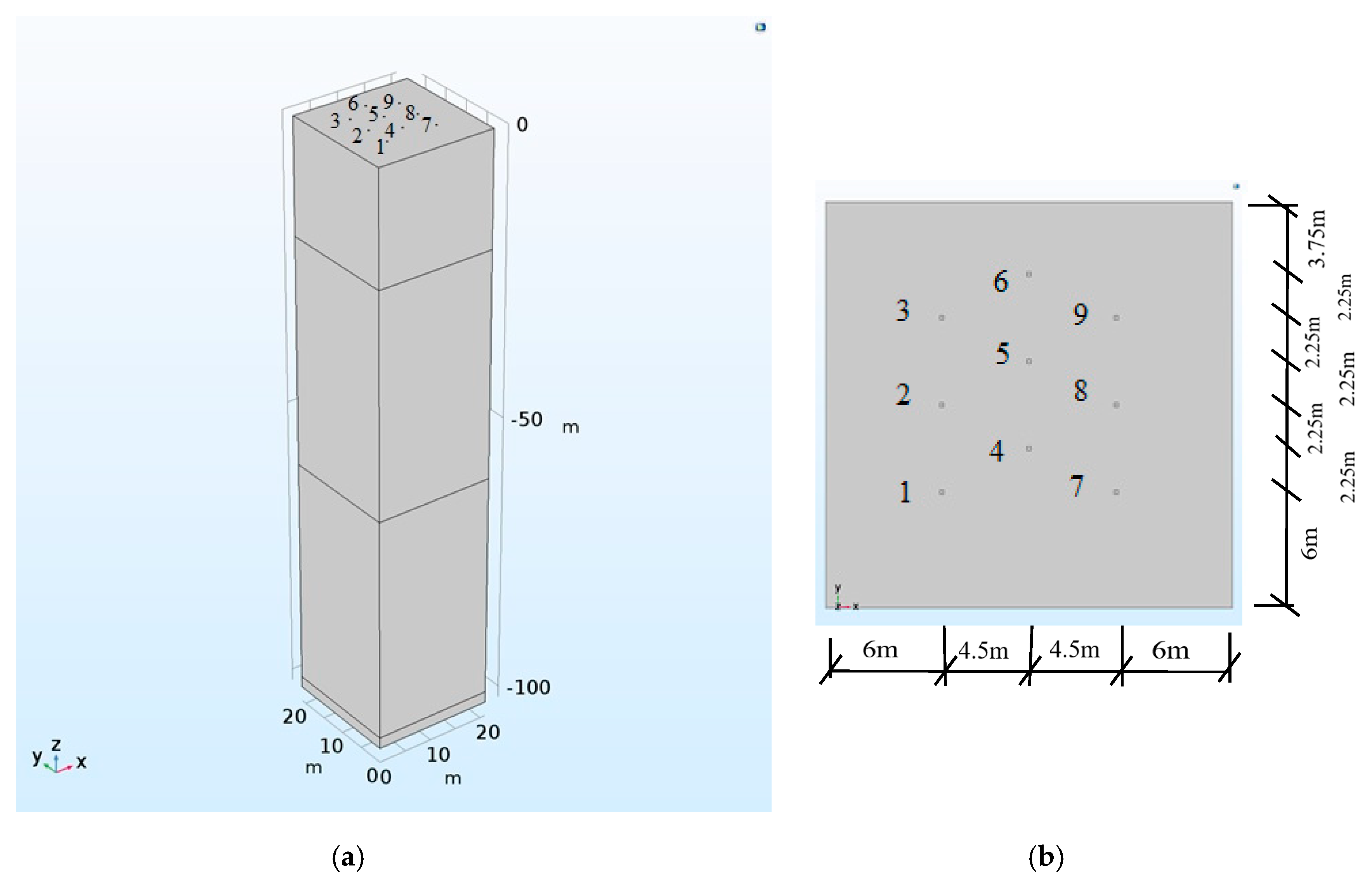
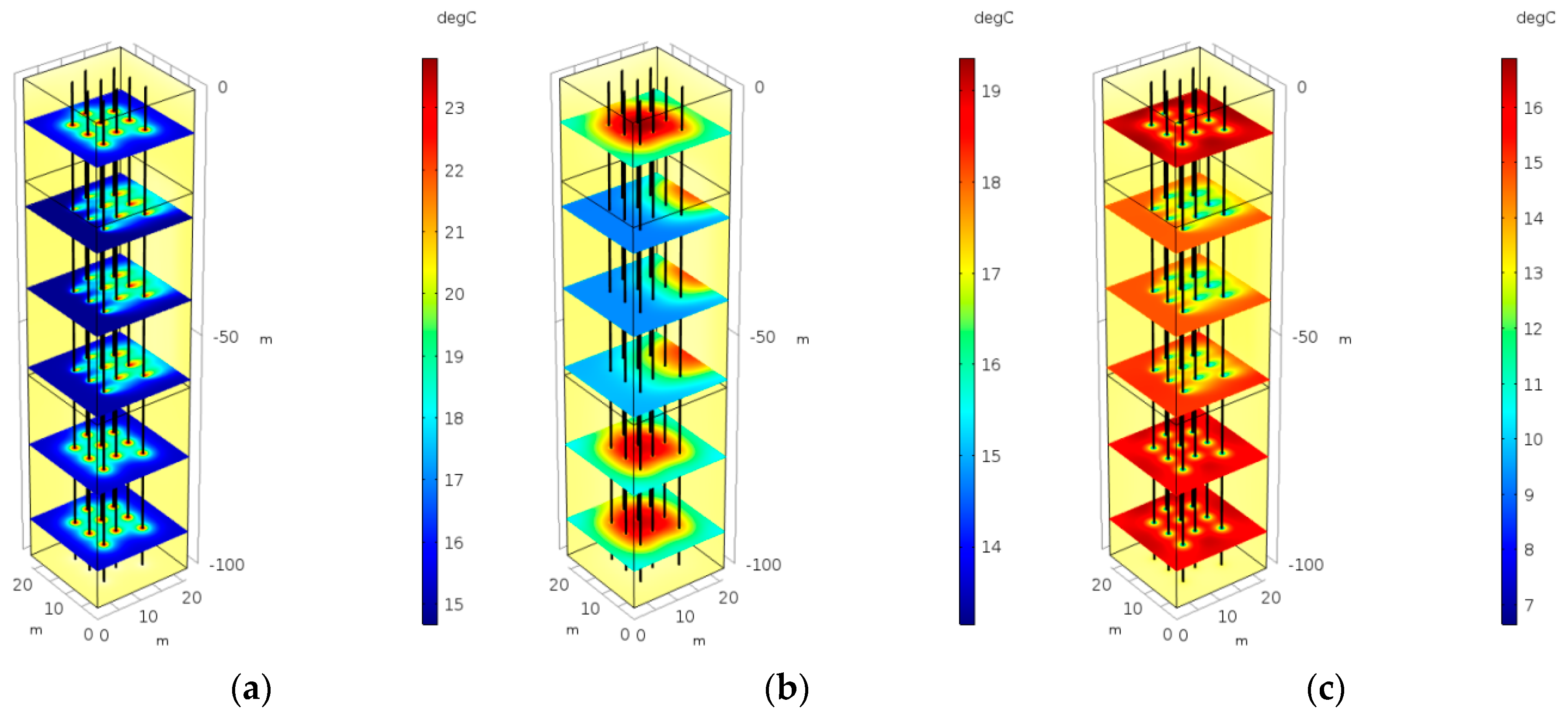
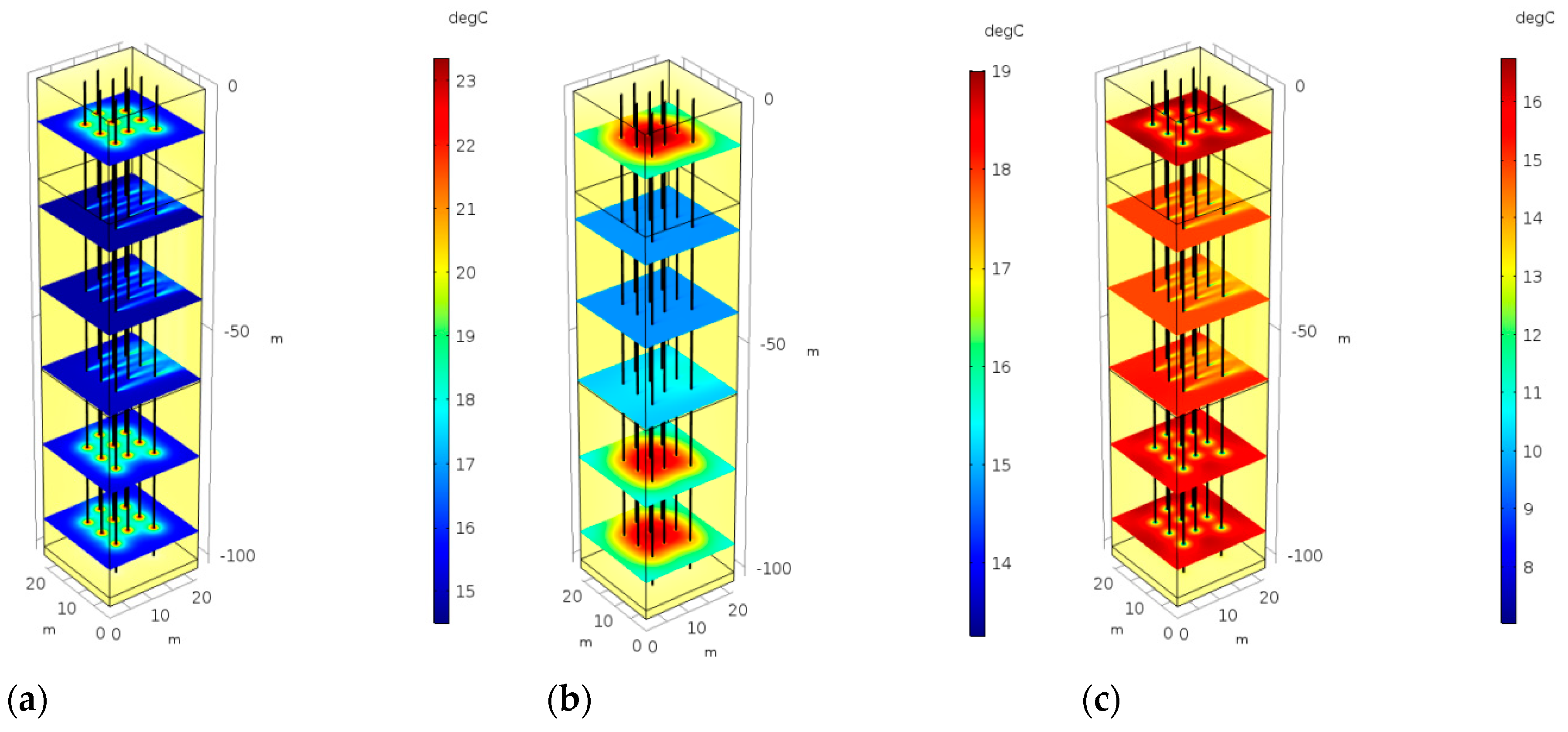
3. Three-Dimensional Numerical Simulation of Influence of Thermal Permeable Coupling of Ground Tube Group on Geothermal Field

Based on the control equation in Section 2.1 of the ground buried tube thermal permeable coupling model and the simplified model of the buried pipe in Section 2.3, the geothermal field coupled with the thermal permeable coupling of the buried pipe group was simulated by the misaligned tube group model.

According to the previous research results, in the case of groundwater permeability, the heat transfer capacity of the misaligned tube group is higher than that of the smoothing tube group, and the permeable effect of the groundwater makes it more obvious. In this paper, a thermal-permeability coupling model of the buried tube group with misaligned arrangement was established. The model length × width × depth = 21 m × 21 m × 102 m (see Figure 7a). The tube group consisted of nine buried pipes. The buried pipe was buried at a depth of 100 meters and the buried pipes were arranged at a distance of 4.5 m (see Figure 7b). The buried pipe passed through three layers, where the first layer was clay, and the second layer was a water-bearing homogeneous pore sandstone. The water flow direction flowed from the hole 1 side to the hole 7 side (Figure 7b), and the third layer was clay.

The initial values of the formation temperature of the buried pipe group thermal permeable coupling model are shown in Table 1. The drilling dimensions and thermal properties of the formation are shown in Table 2.

According to Equations (5) and (6), the groundwater permeable velocity can be calculated by the hydraulic conductivity, k, and the water head, $\nabla H$. The simulation system ran for 360 days, where the 0–120 days circulating fluid flow was 0.16 L/s, the inlet temperature was set to 30 °C, and the ground source heat pump cooling condition was simulated; the 120–240 days circulating fluid flow rate was 0, simulating the shutdown condition; and for 240–360 days, the circulating fluid flow rate was 0.16 L/s and the inlet temperature was set to 6 °C to simulate the heating conditions. The size and thermal property parameters of the formation, grout, and U-tube were the same as the thermal response test in Section 2.4.2.

Discretize the model and the total mesh generation was 850,000. In the borehole domain, it had a minimum mesh size of 0.02 m and a maximum mesh size of 0.15 m. In the formation domain, the mesh sizes were larger than those in the borehole domain, where the minimum mesh size was 0.2 m and the maximum mesh size was 2.5 m. The time step was one day.

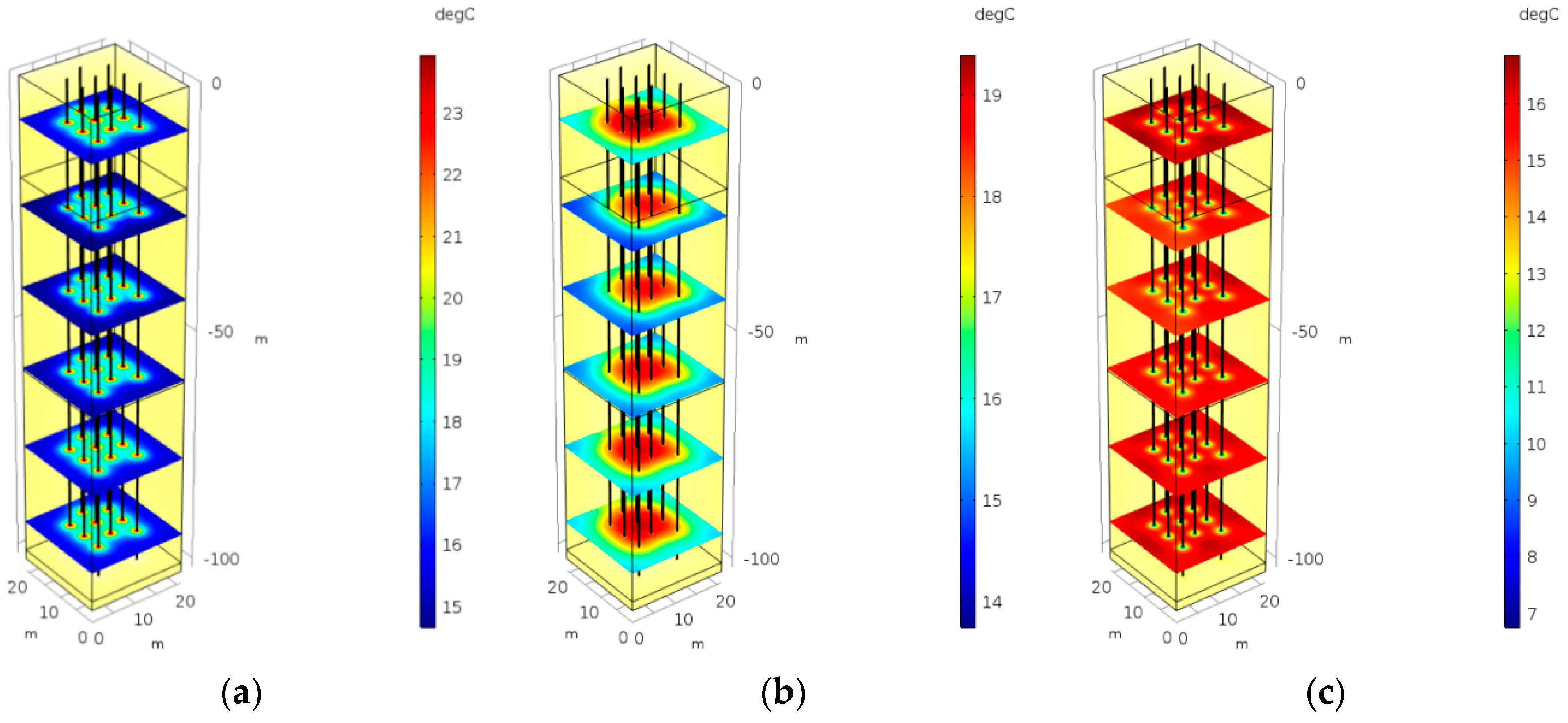
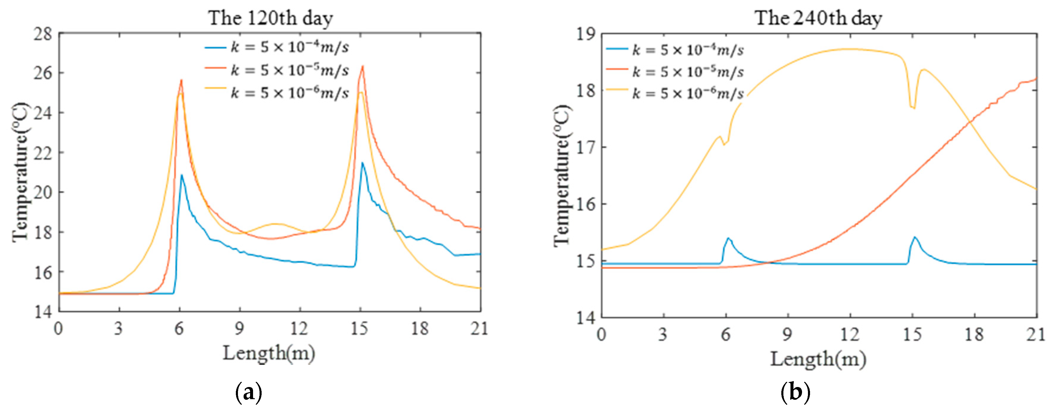
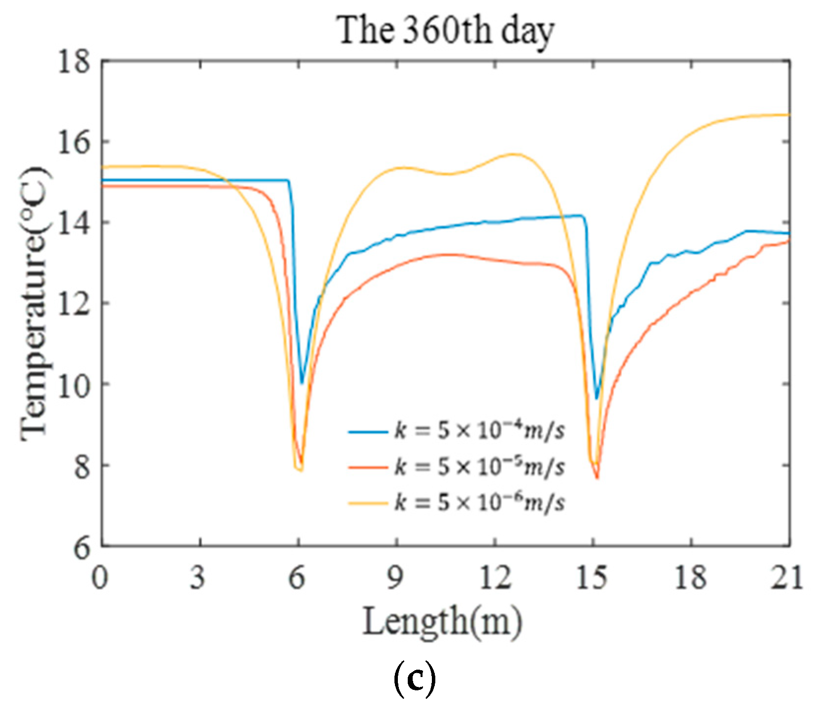
4. Results and Discussion

The head difference ΔH = 0.5 m in the second aquifer, at a different hydraulic conductivity condition of $k=5\times \frac{{10}^{-6}m}{s}, k=5\times \frac{{10}^{-5}m}{s}, k=5\times {10}^{-4}m/s$, after which the simulation calculated the heat removal to the formation for 120 days, stopped for 120 days, and took heat from the formation for 120 days, where the system continuously ran the temperature field in the 360 day formation. Additionally, the effect of the hydraulic conductivity on the temperature field around the buried pipe was studied.

When $k=5\times {10}^{-6}m/s$, the 120 days, 240 days, and 360 days’ formation temperature fields are as shown as Figure 8a–c.

When$k=5\times {10}^{-5}m/s$, the 120 days, 240 days and 360 days’ formation temperature fields are shown in Figure 9a–c.

When $k=5\times {10}^{-4}m/s$, the 120 days, 240 days and 360 days’ formation temperature fields are as shown in Figure 10a–c.

Comparing and analyzing Figure 8, Figure 9 and Figure 10, we observed the following. (1) When the hydraulic conductivity was $k=5\times {10}^{-6}m/s$, the temperature field in the permeable stratum was symmetrically distributed around the borehole. The heat discharged after shutdown was mainly concentrated around the buried pipe, which is beneficial to the formation heat storage. (2) When $k=5\times {10}^{-5}m/s$, the temperature field around the buried pipe in the permeable stratum was offset, and it was distributed in an elliptical shape around the buried pipe. The influence between the buried pipes was small. The heat was transferred to the outside of 9 m with the permeable groundwater. (3) When $k=5\times {10}^{-4}m/s$, the temperature around the buried pipe in the permeable stratum was mainly concentrated in the downstream of the buried pipe, and the heat was transferred to 21 m after the shutdown.

Under different hydraulic conductivity, the temperature value of the connection between the #2 hole and the #8 hole (see Figure 6b) of the 40-meter permeable stratum in the depth of the borehole pipe system after 120 days, 240 days, and 360 days operation was studied and Figure 11 was obtained.

Comparing the analysis of Figure 11a–c, it can be concluded that the misalignment can reduce the mutual influence between the buried pipes. When the hydraulic conductivity is $k=5\times {10}^{-4}m/s$, the temperature outside the buried pipe wall is significantly reduced under the influence of permeable groundwater, and the temperature in the formation returns to the original formation temperature after shutdown.

When the head difference $\nabla H$ is 0.5 m and the hydraulic conductivity $k$ is $5\times {10}^{-6}m/s$, $5\times {10}^{-5}m/s$, and $5\times {10}^{-4}m/s$, respectively, the outlet temperature value of the buried pipe located at the middle of the buried pipe group and Figure 12 can be obtained. When the hydraulic conductivity was $k=5\times {10}^{-4}m/s$, regardless of the heat exhaust condition or the heat extraction condition, the outlet temperature of the buried pipe was more than 1.8 °C lower than the hydraulic conductivity$k=5\times {10}^{-5}\mathrm{m}/\mathrm{s}$, and the permeable groundwater significantly provided the heat exchange efficiency of the buried pipe.

5. Conclusions

In this paper, a new simplified model of buried pipe was proposed. Based on the finite element numerical simulation software COMSOL and the simplified buried pipe model, the same numerical model as the sandbox test and the on-site thermal response test was established using the sandbox test data and the on-site thermal response test data. The results of simulation showed that the simplified ground tube model simulation results agreed well with the experimental data, and the simplified buried tube model improved the meshing efficiency and significantly improved the simulation efficiency.

Based on the simplified buried pipe model, the temperature field in the formation after one year of thermal-permeability coupled heat transfer operation of the buried pipe group under different hydraulic conductivity conditions was studied, and the temperature field distribution of the system under different operating conditions was obtained. By analyzing and comparing the formation temperature field, the influence of groundwater can be neglected only when the head difference is less than 0.5 m and the hydraulic conductivity is less than$k=5\times {10}^{-6}\mathrm{m}/\mathrm{s}$. When the head difference is more than 0.5 m and the hydraulic conductivity is more than $k=5\times {10}^{-5}\mathrm{m}/\mathrm{s}$, the influence of permeable groundwater can effectively avoid the heat accumulation in the formation. The misplaced arrangement of the buried pipes can reduce the mutual influence between the buried pipes. The distribution of temperature fields in the different strata was different, which is closely related to the thermal properties of the formation and the flow of groundwater. When the hydraulic conductivity is more than $k=5\times {10}^{-4}\mathrm{m}/\mathrm{s}$, the flow of groundwater can significantly improve the heat exchange efficiency of the buried pipe.

References

1. Lund, J.W.; Sanner, B.; Rybach, L.; Curtis, R.; Hellstrom, G. Geothermal (groundsource) heat pumps. A world overview. GHC Bulletin 2004, 25, 1–10. [Google Scholar]
2. Bernier, M. Closed-loop ground-coupled heat pump systems. ASHRAE J. 2006, 48, 13–24. [Google Scholar]
3. Nguyen, H.V.; Law, Y.L.E.; Alavy, M.; Walsh, P.R.; Leong, W.H.; Dworkin, S.B. An analysis of the factors affecting hybrid ground-source heat pump installation potential in North America. Appl. Energy 2014, 125, 28–38. [Google Scholar] [CrossRef]
4. Ingersoll, L.R.; Zobel, O.J.; Ingersoll, A.C. Heat Conduction with Engineering, Geological, and Other Applications, Revised ed.; The University of Wisconsin Press: Madison, WI, USA, 1954. [Google Scholar]
5. Li, M.; Lai, A.C.K. Review of analytical models for heat transfer by vertical ground heat exchangers (GHEs): A perspective of time and space scales. Appl. Energy 2015, 151, 178–191. [Google Scholar] [CrossRef]
6. Witte, H.J.L. Geothermal response test with heat extraction and heat injection: Examples of application in research and design of geothermal ground heat exchangers. In Europaischer Workshop uber Geothermische Response Tests; Ecole Poly Technique Federal de Lausanne: Lausanne, Switzerland, 25–26 October 2001. [Google Scholar]
7. Santa, G.D.; Galgaro, A.; Tateo, F.; Cola, S. Modified compressibility of cohesive sediments induced by thermal anomalies due to a borehole heat exchanger. Eng. Geol. 2016, 202, 143–152. [Google Scholar] [CrossRef]
8. Eskilson, P. Thermal Analysis of Heat Extraction Boreholes. Ph.D. Thesis, Lund University, Lund, Sweden, 1987. [Google Scholar]
9. Capozza, A.; De Carli, M.; Zarrella, A. Design of borehole heat exchangers for ground-source heat pumps: A literature review, methodology comparison and analysis on the penalty temperature. Energy Build. 2012, 55, 369–379. [Google Scholar] [CrossRef]
10. Raymond, J.; Therrien, R.; Gosselin, L.; Lefebvre, R. A review of thermal response test analysis using pumping test concepts. Groundwater 2011, 49, 932–945. [Google Scholar] [CrossRef] [PubMed]
11. Zhang, C.X.; Guo, Z.J.; Liu, Y.F.; Cong, X.C.; Peng, D.G. A review on thermal response test of ground-coupled heat pump systems. Renew. Sustain. Energy Rev. 2014, 40, 851–867. [Google Scholar] [CrossRef]
12. Lamarche, L.; Kajl, S.; Beauchamp, B. A review of methods to evaluate borehole thermal resistances in geothermal heat-pump systems. Geothermics 2010, 39, 187–200. [Google Scholar] [CrossRef]
13. Yang, H.X.; Cui, P.; Fang, Z.H. Vertical-borehole ground-coupled heat pumps: A review of models and systems. Appl. Energy 2010, 87, 16–27. [Google Scholar] [CrossRef]
14. Wang, F.H.; Yu, Bin.; Yan, L. Heat transfer analysis of groundwater flow for multi-pipe heat exchanger of ground source heat pump. CIHESC J. 2010, 61, 57–62. [Google Scholar]
15. Wang, H.; Qi, C.; Du, H.; Gu, J. Thermal performance of borehole heat exchanger under groundwater flow: A case study from Baoding. Energy Build. 2009, 41, 1368–1373. [Google Scholar] [CrossRef]
16. Chiasson, A.D.; Rees, S.J.; Spitler, J.D. A preliminary assessment of the effects of groundwater flow on closed-loop ground-source heat pump systems. ASHRAE Trans. 2000, 106, 380–393. [Google Scholar]
17. Fan, R.; Jiang, Y.; Yao, Y.; Deng, S.; Ma, Z. A study on the performance of a geothermal heat exchanger under coupled heat conduction and ground-water advection. Energy 2007, 32, 2199–2209. [Google Scholar] [CrossRef]
18. Lu, G. Analysis of effect of groundwater seepage on heat transfer in under ground heat exchanger. Fujian Construct. Sci. Technol. 2011, 1, 62–63, 74. [Google Scholar]
19. Luo, J.; Tuo, J.; Huang, W.; Zhu, Y.; Jiao, Y.; Xiang, W.; Rohn, J. Influence of groundwater levels on effective thermal conductivity of the ground and heat transfer rate of borehole heat exchangers. Appl. Therm. Eng. 2018, 128, 508–516. [Google Scholar] [CrossRef]
20. Spitler, J.D.; Gehlin, S.E.A. Thermal response testing for ground source heat pump systems – An historical review. Renew. Sustain. Energy Rev. 2015, 50, 1125–1137. [Google Scholar] [CrossRef]
21. Diao, N.R.; Li, Q.Y.; Fang, Z.H. An analytical solution of the temperature response in geothermal heat exchangers with groundwater advection. J. Shandong Univ. Archit. Eng. 2003, 18, 1–5. [Google Scholar]
22. Diao, N.; Li, Q.; Fang, Z. Heat transfer in ground heat exchangers with groundwater advection. Int. J. Therm. Sci. 2004, 43, 1203–1211. [Google Scholar] [CrossRef]
23. Molina-Giraldo, N.; Bayer, P.; Blum, P. Evaluating the influence of thermaldispersion on temperature plumes from geothermal systems using analytical solutions. Int. J. Therm. Sci. 2011, 50, 1223–1231. [Google Scholar] [CrossRef]
24. Wagner, V.; Blum, P.; Kubert, M.; Bayer, P. Analytical approach for groundwaterinfluencedthermal response tests of grouted borehole heat exchangers. Geothermics 2013, 46, 22–31. [Google Scholar] [CrossRef]
25. Wagner, V.; Bayer, P.; Bisch, G.; Kubert, M.; Blum, P. Hydraulic characterizationof aquifers by thermal response testing: Validation by large scale tank laboratoryand field experiments. Water Resour. Res. 2014, 50, 1–15. [Google Scholar] [CrossRef]
26. Aranzabal, N.; Martos, J.; Montero, Á.; Monreal, L.; Soret, J.; Torres, J.; García-Olcina, R. Extraction of thermal characteristics of surrounding geological layers of a geothermal heat exchanger by 3D numerical simulations. Appl. Therm. Eng. 2016, 99, 92–102. [Google Scholar] [CrossRef]
27. Guan, X. China’s ground source heat pump development and utilization prospects. China Sci. Technol. Inf. 2010, 21, 21–23. [Google Scholar]
28. Yavuzturk, G. Modeling of Vertical Ground Loop Heat Exchangers for Ground Source Heat Pump Systems; Oklahoma State University: Stillwater, OK, USA, 1999. [Google Scholar]
29. Li, X.G.; Zhao, J.; Zhou, Q. Numerical simulation on the ground temperature field around U pipe underground heat exchanger. J. Acta Energ. Sol. Sin. 2004, 25, 703–707. [Google Scholar]
30. Gao, Q.; Li, M.; Yan, Y. Effect on ground source field heat transfer of original earth temperature and configuration of multi-borehole. J. Therm. Sci. Technol. 2005, 4, 34–40. [Google Scholar]
31. Zhao, J.; Wang, H.J. Numerical simulation on heat transfer characteristics of soil around compact pile-buried underground heat exchangers. J. HV AC 2006, 36, 11–14. [Google Scholar]
32. Jia, Y.B.; Wang, Y. Comparative analyses on 2D and 3D buried tube-group heat transfer models in GCHP system. J. Grad. Univ. Chin. Acad. Sci. 2013, 30, 311–316. [Google Scholar]
33. Yang, G.J.; Guo, M. Research on group arrangement method of ground heat exchanger under coupled thermal conduction and groundwater seepage conditions. Renew. Energy Resour. 2014, 32, 1182–1187. [Google Scholar]
34. Li, P.; Li, M.; Ma, W.; Xiao, L. Temperature responses of ground heat exchanger clusters based on full-scale line-source solution. J. Central South Univ. 2017, 48, 2818–2822. [Google Scholar]
35. Han, C.J.; Yu, X. Sensitivity analysis of a vertical geothermal heat pump system. Appl. Energy 2016, 170, 148–160. [Google Scholar] [CrossRef] [Green Version]
36. Oberdorfer, P.; Hu, R.; Rahman, M.; Holzbecher, E.; Sauter, M.; Mercker, O.; Pärisch, P. Coupled Heat Transfer in Borehole Heat Exchangers and Long Time Predictions of Solar Rechargeable Geothermal Systems; COMSOL: Milan, Italy, 2013. [Google Scholar]
37. Yu, Y.; Liu, G.; Jiang, B. Finite element analysis of ground source heat pump based on non-isothermal pipe flow. J. Zhejiang Univ. Sci. Technol. 2015, 27, 218–224. [Google Scholar]
38. Beier, R.A.; Smith, M.D.; Spitler, J.D. Reference data sets for vertical borehole ground heat exchanger models and thermal response test analysis. Geothermics 2011, 40, 79–85. [Google Scholar] [CrossRef]
Figure 1. Schematic diagram of the buried pipe.
Energies 12 03698 g001
Figure 2. Borehole with U-pipe and its simplified model showing the relative position of the buried pipes.
Energies 12 03698 g002
Figure 3. Sandbox test verification.
Energies 12 03698 g003
Figure 4. Thermal response tester.
Energies 12 03698 g004
Figure 5. The results of the on-site thermal response test simulation.
Energies 12 03698 g005
Figure 6. On-site thermal response test verification.
Energies 12 03698 g006
Figure 7. The model of buried pipe group physical model: (a) three dimensions and (b) cross section.
Energies 12 03698 g007
Figure 8. When k = 5 × 10 6 m / s , the formation temperature field at different times: (a) 120 days; (b) 240 days; (c) 360 days.
Energies 12 03698 g008
Figure 9. When k = 5 × 10 5 m / s , the formation temperature field at different times: (a) 120 day; (b) 240 days; (c) 360 days.
Energies 12 03698 g009
Figure 10. When k = 5 × 10 4 m / s , formation temperature field at different times: (a) 120 days; (b) 240 days; (c) 360 days.
Energies 12 03698 g010
Figure 11. Temperature at the junction of #2 and #8 holes in the −40 m section at different times: (a) 120 days; (b) 240 days; (c) 360 days.
Energies 12 03698 g011aEnergies 12 03698 g011b
Figure 12. Effect of hydraulic conductivity on outlet temperature.
Energies 12 03698 g012