Reactive Power Optimization of a Distribution System Based on Scene Matching and Deep Belief Network

Abstract

With a large number of distributed generators (DGs) and electrical vehicles (EVs) integrated into the power distribution system, the complexity of distribution system operation is increased, which arises to higher requirements for online reactive power optimization. This paper proposes two methods for online reactive power optimization, a scene-matching method based on Random Matrix (RM) features and a deep learning method based on Deep Belief Network (DBN). Firstly, utilizing the operation and ambient Big Data (BD) of the distribution system, we construct the high-dimension Random Matrices and extract 57 state features for the subsequent scene-matching and DBN training. Secondly, the feature-based scene-matching method is proposed. Furtherly, to effectively deal with the uncertainty of DGs and to avoid the performance deterioration of the scene-matching method under a new unknown scene, the DBN-based model is constructed and trained, with the former features as the inputs and the conventional reactive power control solutions as the outputs. This DBN model can learn the nonlinear complicated relationship between the system features and the reactive power control solutions. Finally, the comprehensive case studies have been conducted on the modified IEEE-37 nodes active distribution system, and the performances of the proposed two methods are compared with the conventional method. The results show that the DBN-based method possesses the better performance than the others, and it can reduce the network losses and node voltage deviations obviously, even under the new unknown and unmatched scenes. It does not depend on the distribution system model and parameters anymore and can provide online decision-making more quickly. The discussions of the two methods under different DG penetrations and the historical data volume were given, verifying the adaptability, robustness and generalization ability of the DBN-based method.

1. Introduction

The reactive power optimization of the distribution network can reduce the power losses and improve the voltage quality and the economical operation of a distribution network [1,2,3,4]. By regulating the reactive power compensation equipment such as fixed shunt capacitor banks, online tap changing transformers and SVCs (static VAR compensators), etc. [5,6], the reactive power optimization can realize reasonable distribution of reactive power in the distribution network and reduce the power losses and node voltage deviations. The algorithm is a key issue of the reactive power optimization of the distribution network [7]. The nonlinear characteristic is prominent in reactive power optimization and is composed of multivariate, multi-constraint, discrete variables and continuous variables. The conventional optimization methods are dependent on the model and parameters of the distribution network, which have obvious disadvantages of poor convergence and stability. And in practical application, the optimization computational cost is large and the decision-making time is long, so it becomes more difficult to apply these methods to the real-time control requirements of the complicated active distribution system [8,9]. In recent years, some of the heuristic intelligent algorithms have been widely developed for reactive power optimization [10,11,12,13], and although these methods can process the discrete variables accurately, the initial values of these algorithms are adopted randomly, which may extend the computation time, and tend to fall into local minima.

Recently, distributed generators (DG) and electric vehicles (EV) are widely being used, although the power flow of the distribution network is affected by the intermittency and randomness of DGs and EVs, which increased the difficulty of reactive power optimization of distribution networks [14,15]. Most of the existing literature dealt with the aspects of model simplification and optimization method improvement [16]. In [17], Zheng et al. presented a fully distributed reactive power optimization algorithm that can obtain the global optimum solution of nonconvex problems for distribution networks without requiring a central coordinator. In [18], considering the uncertain fluctuation of the PV output and the load power, a robust optimal allocation of decentralized reactive power compensation devices model for a three-phase four-wire low voltage distribution network (LVDN) was proposed. Although the computational efficiency and convergence of reactive power optimization were improved, the limitations of conventional algorithms still existed. It is important to explore the reactive power optimization method of the distribution network which is not dependent on the models and parameters to ensure the stability and quality of distribution system operation.

Meanwhile, with the improvements of power system sensing and communication, mass operation information can be accessed through various measurement sensors, which brings an opportunity to the innovation of reactive power optimization methods. It is true that data mining and analysis is the key technology. Nowadays, data mining technology is applied to power systems, e.g., Liu et al. introduced a distributed load forecasting method based on local weather information [19], Ouyang et al. proposed a data-driven deep learning framework to forecast the short-term power load [20], and Zhu et al. employed four featured deep learning approaches in forecasting the EVs charging load from the charging station perspective [21].

Although data-driven methods are mainly used in the field of load forecasting as above, relevant studies have confirmed the possibility of applying it to reactive power optimization. In [22], Sheng et al. put forward a big data modeling method for the reactive power optimization based on the theory of the large dimensional random matrix. In [23], Ji et al. proposed a reactive power optimization method based on load distribution matching and the entropy weight method. They matched load scenarios from the historical database that are similar to the current optimization time and selected the optimal control scheme from the historical optimization scheme by entropy weight method. In [24], Cao et al. conducted a study of transient voltage stability analysis based on convolutional neural networks and proposed a reactive power compensation decision optimization algorithm via a deep reinforcement learning approach. In [25], Salles et al. investigated the application of support vector machines (SVMs) to minimize system losses and to maintain an acceptable voltage profile of distribution systems. They used voltage/current measurements provided by active and reactive monitors to control reactive power compensation equipment without the need to perform retraining or repeat optimization simulations.

Reactive power optimization is a complex high-dimensional nonlinear problem. In recent years, thanks to the developments on Big Data (BD) and Artificial Intelligence (AI) technologies, represented by deep learning (DL), data-driven AI-based online decision-making becomes possible [26]. Useful information can be found out by the AI analysis method based on data driven from the historical data and analyzing the implicit rules between the inputs and outputs directly [27,28]. Random Matrix (RM) theory is a universal method for BD analysis, and does not require detailed physical models [29]. Based on the overall consideration of historical data and real-time data, this method has advantages in interpreting the complex system from a high-dimensional point-of-view [30]. The Deep Belief Network (DBN) possesses the benefits of a strong feature extraction ability, simple model structure, being easy to train and a fast convergence speed [31,32]. It is considered as an effective method to solve the complex high-dimensional nonlinear mapping problems [33].

The motivation of this paper is to propose the Big Data (BD) and AI-based distribution network reactive power optimizing method, to take advantage of historical operation BD through Deep Learning, and also to effectively deal with the uncertainty of DGs. Firstly, the high-dimension Random Matrices are constructed, 57 state features are extracted, and the feature-based scene-matching method for reactive power optimization is proposed. Furtherly, to effectively deal with the uncertainty of DGs and to avoid performance deterioration under the new unknown scenes, the DBN-based model is constructed and trained. Lastly, comprehensive case studies were conducted on the IEEE-37 test bed, the performances of these two proposed methods and the conventional method are compared, and the discussions about the influence of the historical data volume, and the adaptability under high DG penetrations, are given.

The main contributions can be summarized as follows:

(1)

Utilizing the operation data and ambient data of a distribution network, this paper proposed two kinds of approaches to construct the high-dimensional Random Matrix and extracted 57 statistical features. These statistical state features of the current scene under optimization were matched with those in the historical database, and the control solution of the matching scene was applied to the current scene directly for reactive power control and voltage management.

(2)

A Deep Belief Network (DBN) with one input layer, two hidden layers and one output layer has been constructed and optimized, with the 57 statistical state features as inputs and the conventional optimized control solutions as output. The historical data were used to train DBN to learn the nonlinear relationship between system features and reactive power control solutions.

(3)

Comprehensive case studies were carried out on the modified IEEE-37 active distribution network, and the optimization effects of the scene-matching method and the data-driven DBN method were compared with the conventional optimization method, and the effects under different historical data volumes and different DG penetrations were also investigated, verifying the effectiveness and excellent generalization ability of the proposed DBN-based model.

The rest of this paper is organized as follows: Section 2 introduces the related theory of RM and DBN. Section 3 introduces the feature-based scene-matching method by constructing RM. Section 4 proposes the data-driven DBN-based method for reactive power optimization. The case studies are given in Section 5. Section 6 discusses the effects of two methods under different historical data volumes and different DG penetrations. Section 7 deduces the conclusions.

2. Related Theory and Work

2.1. Random Matrix Theory

The random matrix (RM) can process independent and identically distributed data. RM has no prerequisites on the data distribution of the source data (such as the Hermitian matrix satisfying the Gaussian distribution, etc.), and only requires a large-enough volume of data (not infinite) [29]. The empirical spectral distribution function of a random matrix has many excellent properties, such as the Single Ring Law, Marchenko–Pastur Law and so on [30]. This paper is mainly based on the Single Ring Law.

Let the random matrix $\mathit{X}\in {\mathit{C}}^{N\times M}$ be an N × M-dimensional complex matrix, and then the matrix X shall be normalized and converted to the standard non-Hermitian matrix $\tilde{\mathit{X}}\in {\mathit{C}}^{N\times M}$, where the transformed row vectors have a mean of $\overline{{\tilde{\mathit{x}}}_i}=0$ and a standard deviation of $\sigma ({\tilde{\mathit{x}}}_i)=1$. To obtain the eigenvalues of the random matrix, for multiple standard non-Hermitian random matrices ${\tilde{\mathit{X}}}_i$(I = 1,2, …, L), firstly we need to transform $\tilde{\mathit{X}}$ into a singular value equivalent matrix ${\tilde{\mathit{X}}}_u\in {\mathit{C}}^{N\times N}$, then define the matrix product as

$$\mathit{Z}={\displaystyle \prod _{i=1}^L{\tilde{\mathit{X}}}_{\mathit{u},i}},$$

(1)

where ${\tilde{\mathit{X}}}_{\mathit{u},i}$ is the singular value equivalent matrix of ${\tilde{\mathit{X}}}_i$. The matrix product Z can be converted to the standard matrix product $\tilde{\mathit{Z}}$. According to the Single Ring Law, the eigenvalues of $\tilde{\mathit{Z}}$ in the complex plane will be roughly distributed between two rings. The outer ring radius is 1, and the inner ring radius is ${\left(1-c\right)}^{2/L}$, where $c=N/M\in \left(0,1\right]$. The image of the Single Ring Law is shown in Figure 1, where L = 1, N = 80, and M = 200.

The linear eigenvalue statistic (LES) can reflect the distribution of eigenvalues of a random matrix. For matrix $\tilde{\mathit{Z}}$, the linear eigenvalue statistic is defined as

$${\varsigma }_N\left(\phi \right)={\displaystyle \sum _{i=1}^N\phi \left({\lambda }_i\right)},$$

(2)

where ${\lambda }_i\left(i=1,2,3\dots ,N\right)$ are the eigenvalue of matrix $\tilde{\mathit{Z}}$ and $\phi (\cdot )$ is the test function. Different linear eigenvalue statistics can be obtained by selecting different test functions.

Each eigenvalue of the matrix product $\tilde{\mathit{Z}}$ is a complex function of the random matrix X. The fluctuation of the eigenvalues can reflect the fluctuation of the matrix elements, and thus reflect the operating state of the corresponding physical system.

2.2. Deep Belief Network (DBN)

The DBN is a deep learning network composed of a basic unit of the Restricted Boltzmann Machine (RBM), which possesses powerful feature extraction capabilities.

2.2.1. Restricted Boltzmann Machine

RBM is a typical probability generation model which has strong unsupervised learning ability, and its input layer neurons and hidden layer neurons are all binary variables. As illustrated in Figure 2, RBM is a bi-level neural network which is composed of n visible nodes and m hidden nodes, with no connection within the layer and full connection between the layers.

RBM is a kind of probability model [34]. For a training sample set with the capacity s, S = {v1, v2, …, vs}, the training goal of RBM is to adjust the parameters of RBM iteratively and maximally fit a given training sample [35]. Based on the optimization theory, it is equivalent to maximize the log-likelihood function $L(\theta )$ of RBN on the training set. Then the model parameter $\theta$ can be solved as follows:

$${\theta }^{*}=\arg \max L(\theta )=\arg \max {\displaystyle \sum _{k=1}^l\log P(v^k|h,\theta )}.$$

(3)

The training of RBM can be performed with the contrastive divergence (CD) algorithm, which takes the first partial derivative of $L(\theta )$ with respect to $\theta$ and then seeks the optimal parameters according to the stochastic gradient descent principle. The derivation process is based on the Gibbs sampling method, which takes a training sample to initialize the visual layer nodes v and conducts the Gibbs sampling k times alternatively, then uses the values of $P(h|v^{(k)})$, $v^{(k)}$ obtained by the k-th sampling to approximate the partial derivative values of $L(\theta )$, then update the parameters according to Equations (4)–(6) to complete the training of a single RBM.

$$w=\rho w+\eta [p(H_i=1|v^{(0)})\cdot v_j^{(0)}-p(H_i=1|v^{(k)})\cdot v_j^{(k)}],$$

(4)

$$a=\rho a+\eta (v^{(0)}-v^{(k)}),$$

(5)

$$b=\rho b+\eta [p(h=1|v^{(0)})-p(h=1|v^{(k)})],$$

(6)

where $\rho$ is the momentum, $\eta$ is the learning rate and k = 1 in this paper.

2.2.2. The Structure and Training Method of DBN

As illustrated in Figure 3, the DBN is composed of several layers of RBM and one layer of the BP neural network in a stacked way. It is a probabilistic generation model, which is to enable the entire neural network to generate data according to the maximum probability through training the weights between neurons.

The training process of DBN is divided into two steps: Bottom-up unsupervised pre-training and top-down supervised parameter fine-tuning [32]. Firstly, unsupervised pre-training is carried out from the input layer to the top hidden layer. This process only needs to input features of the training set to train the stacked RBM layer-by-layer and initialize the parameters of the entire DBN structure. Next, all the RBMs are unfolded to synthesize a complete neural network with the output layer added to the end sequentially. The error back propagation algorithm is used to adjust the parameters of the entire DBN structure from top most to bottom. This process requires inputting label data, which is called supervised fine-tuning. This two-stage training method initializes the network by an unsupervised greedy learning algorithm, which effectively reduced the space of parameter optimization and the training time for supervised fine-tuning.

3. Scene-Matching Method Based on Random Matrix and Features

In the reactive power optimization of a distribution network, when the volume of the operating data accumulated in the historical database becomes large enough, and the operating scenes are sufficient, then the control solution corresponding to the current scene may always be included in the historical database. Therefore, for the system scene under optimization, the optimal control solution can be determined by matching the current scene with the historical database, and the control solution of the most similar and matching scene can be used directly to the current scene.

The features of the distribution network scene are complicated, and this paper combines random matrix theory to process and analyze these features. One of the key problems of reactive power optimization based on RM is how to construct the high-dimensional random matrix and extract state features. Therefore, based on the current data and historical data, this section calculated the corresponding features, and then selected the scenes with similar features at the current time point from the historical database to determine the reactive power optimization solution.

3.1. Distribution System Random Matrix Modeling

Combined with the time series features of various data in the distribution system, a random matrix for scene-matching and reactive power optimization based on a time series can be constructed as follows.

Firstly, by analyzing the data sources affecting reactive power optimization and voltage distribution, four kinds of electric quantity state data (load power, photovoltaic (PV) power, wind turbine (WT) power and charging power of EV) and three kinds of environmental data (temperature, solar radiation intensity and wind speed) are selected to form the random data source of distribution network. Then an $N\times M$ dimension random matrix $\mathit{X}$ is constructed by sampling data of various distribution networks based on time series, where N is the number of state variables and M is the length of the time series.

For the different types of data sources, this section proposes two kinds of approaches to construct Random Matrices.

1.

Construction of the First Kind of Random Matrix

Taking the load random matrix as an example, this part introduced the construction method of the first kind of random matrix. The load random matrix is a random matrix with the load power in the grid as the elements. To satisfy the requirements of constructing RM, the column number (time points) should be far greater than the row number (state variables), at least two times and more. The largest load RM in this paper has 30 loads, so we selected 60 time point data with a 1 min interval before the time point under optimization, to construct the RM. If the interval is too long, the time span became too long, and the features cannot reflect the current status of the distribution network, and if the interval is too short, the features cannot depict the varying trends. Comprehensive experiments have been done and found that 60 time point data with a 1 min interval are most appropriate, and data within 1 h before the time point under optimization can not only reflect the current status, but also depict the varying trends of the network. In the realistic distribution network, different data sources have different sampling intervals, for example the smart meters of the loads and the EV charger upload data every 15 min, but the DGs such as PVs upload data every minute or every five minutes. In order to obtain every minutes’ data, we used the curve fitting and interpolation techniques.

Assuming that the number of load nodes in the distribution network is N, the active powers of 60 min before sampling time t are chosen to represent the load within one hour before sampling time, then the load change of load node i at sampling time t can be expressed as row vector ${\mathit{P}}_{it}$ in a time series:

$${\mathit{P}}_{it}=(p_{i,1}^t,p_{i,2}^t,p_{i,3}^t,\cdot \cdot \cdot ,p_{i,60}^t).$$

(7)

For a power network with N load nodes, the load variation of all load nodes at sampling time t can be expressed by a random matrix ${\mathit{P}}_t\in {\mathit{C}}^{N\times 60}$:

$${\mathit{P}}_t={\left[\begin{array}{c}{\mathit{P}}_{1t}\\ {\mathit{P}}_{2t}\\ ⋮\\ {\mathit{P}}_{Nt}\end{array}\right]}_{\left(N\times 60\right)}.$$

(8)

2.

Construction of the Second Kind of Random Matrix

Due to the small number of state variables such as DG, EV random load, temperature, solar radiation intensity and wind speed, the random matrix model constructed by the first method will not reflect the current scene features well, so the extended random matrix method is needed [29,30].

Taking the photovoltaic random matrix as an example, this part introduced the construction method of the second kind of random matrix. Assuming that there are x photovoltaic power station in the distribution system, the number of state variables that can be measured is x. The photovoltaic power of 60 minutes before the sampling time t was selected to represent the output of photovoltaic within one hour before the sampling time, and the matrix of PV can be constructed according to the time series at the sampling time t. Then the matrix was extended. Firstly, the matrix $\mathit{P}{\mathit{v}}_t$ is copied k times to get the matrix $\mathit{P}{{\mathit{V}}_t}^{\prime }\in {\mathit{C}}^{\left(x\times k\right)\times 60}$, as shown in Equation (9),

$$\mathit{P}{{\mathit{V}}_t}^{\prime }={\left[\begin{array}{c}\mathit{P}{\mathit{v}}_t\\ \mathit{P}{\mathit{v}}_t\\ ⋮\\ \mathit{P}{\mathit{v}}_t\end{array}\right]}_{\left(x\times k\right)\times 60},$$

(9)

where $k=\left[N/x\right]$, square brackets [ ] represents k is the largest integer that not exceeding the numerical value in (N/x). By adjusting the ratio of rows to columns, it is found that when the number of columns is M = 60 and the number of rows is adjusted to 20, a more accurate asymptotic convergence result can be observed, so N is taken as 20 here.

To construct the random matrix and eliminate the correlation of repetitive data, random noise is also introduced into matrix $\mathit{P}{{\mathit{V}}_t}^{\prime }$. Each element of matrix $\mathit{P}{{\mathit{V}}_t}^{\prime }$ is multiplied by random factors within 0.95–1.05 to reduce the interference of the correlation of matrix data on the results, and finally, the random matrix $\mathit{P}{\mathit{V}}_t\in {\mathit{C}}^{(x\times k)\times 60}$ is constructed. The results show that the influence of the random noise on the eigenvalue distribution of the matrix can be neglected.

Similarly, the random matrix construction method is the same for the electrical quantities such as wind power generation, electric vehicle charging power and non-electrical quantities such as temperature, solar radiation intensity and wind speed. Details of random matrix processing and the eigenvalue distribution based on the Single Ring Law can be referred to [29,30].

3.2. Feature Extraction

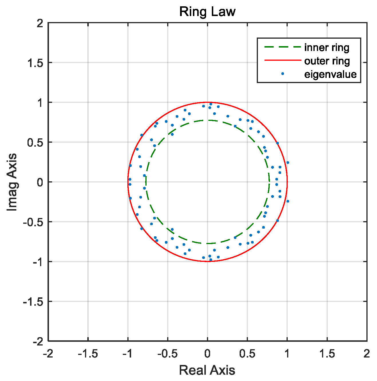
The distribution of the eigenvalues of random matrices varies at different moments, which will change with the operating state of the grid. Since the randomness of a single eigenvalue of a matrix cannot reflect this characteristic, a linear eigenvalue statistic is introduced to reflect the statistical characteristics of eigenvalues and, quantitatively, to describe the state features of a system at a certain moment.

In this section, according to the Single Ring Law, the six statistical indices are defined as mean spectral radius $k_{MSR}$, maximum spectral radius $R_{\max }$, minimum spectral radius $R_{\min }$, outer eigenvalue ratio P₁, upper eigenvalue ratio P₂ and inner eigenvalue ratio P₃, where P₁ to P₃ are used to measure the distribution features of eigenvalues of random matrices outer, on or inner to the dedicated Ring belt (see Figure 1). In order to compare the size of the random matrix conveniently and reflect the fluctuation of a sample, modulus d and the variance Var of random matrix $\mathit{X}$ are also used.

Four electrical data sets (load power, photovoltaic output power, wind turbine output power and EV charging power) and three environmental data sets (temperature, irradiation and wind speed) are selected to construct random matrices, and their eight state features are calculated. Since the total load of the system at current moment can better reflect the system operation, we added the total load as one feature. So, a total of $7\times 8+1=57$ features are extracted at this time. The definitions of these features are shown in Appendix A in detail.

3.3. Scene-Matching Method

The status of the distribution system can be better characterized by these features at that moment. And scene matching is carried out by comparing the similarity of the 57 features. When we want to find the most similar scene to the system under optimization from the historical database, it is necessary to compare the overall deviation between these comprehensive features. The smaller the overall deviation, the higher the similarity. Therefore, the overall deviation between the scene to be optimized and the scene at time t in the historical database is defined as

$$Z_t={\displaystyle \sum _{i=1}^p{k}_i\times {\left(f_i-f{b^t}_i\right)}^2},$$

(10)

where, p is the number of features, $f_i$ is the i-th feature of the time to be optimized, $f{b^t}_i$ is the i-th feature at the time of t in the history of distribution network, and $k_i$ is the weight corresponding to the i-th feature. In this paper, the variance contribution rate of the i-th feature is defined as its weight.

According to Equation (10), the historical scene corresponding to the smallest deviation is the most similar one to the scene under optimization, and the scene matching is realized. The reactive power control solution of the most similar scene is utilized to the current scene directly to control the reactive power and manage the voltages.

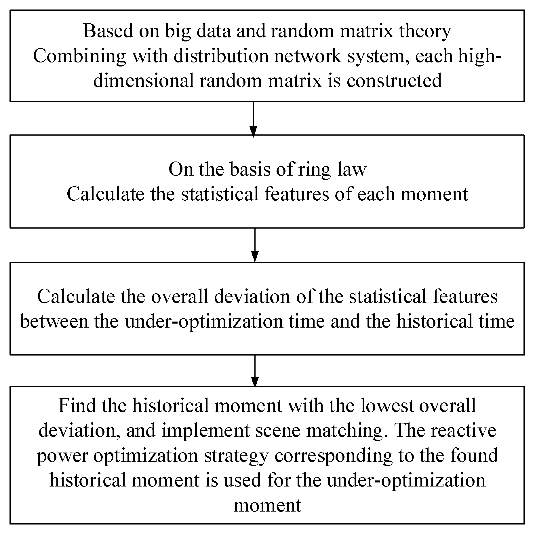
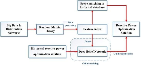
3.4. Scene-Matching Procedure

In summary, the reactive power optimization process of the distribution system based on random matrix theory and the scene matching is shown in Figure 4.

4. DBN-Based Model

In this section, the DBN-based reactive power optimization model is proposed. If the feature of the distribution network system is V and the corresponding reactive power optimization solution is Y, then the reactive power optimization problem of distribution network can be transformed into the searching mapping of $\mathit{V}\to \mathit{Y}$. The DBN is especially suitable for fast and accurate solutions of this kind of problems.

4.1. Construction of the Input Feature Set

One of the key issues of the optimization methods of the distribution network based on deep learning is the construction of the input feature set.

This construction should meet three requirements: The physical meaning is clear, the system dynamic characteristics are presented and the inputs are comprehensive and accessible. The DGs and EV charging stations are affected by weather conditions, temperature and irradiation intensity, etc., so they have strong randomness which results in the operation data of the distribution networks change periodically and present random distribution features. In this paper, 57 features extracted in Section 3.2 are used as the input feature set of DBN in the visible layer. The specific feature variables are shown in

Table A1. 57 features extracted from random matrix.

Index	Features	Index	Features
1	Mean spectral radius of load matrix	30	The ratio of eigenvalues of load matrix in the small circle
2	Mean spectral radius of ev matrix	31	The ratio of eigenvalues of ev matrix in the small circle
3	Mean spectral radius of pv matrix	32	The ratio of eigenvalues of pv matrix in the small circle
4	Mean spectral radius of wind matrix	33	The ratio of eigenvalues of wind matrix in the small circle
5	Mean spectral radius of light intensity matrix	34	The ratio of eigenvalues of light intensity matrix in the small circle
6	Mean spectral radius of temperature matrix	35	The ratio of eigenvalues of temperature matrix in the small circle
7	Mean spectral radius of wind speed matrix	36	The ratio of eigenvalues of wind speed matrix in the small circle
8	Variance of load matrix	37	The ratio of eigenvalues of load matrix outside the large circle
9	Variance of ev matrix	38	The ratio of eigenvalues of ev matrix outside the large circle
10	Variance of pv matrix	39	The ratio of eigenvalues of pv matrix outside the large circle
11	Variance of wind matrix	40	The ratio of eigenvalues of wind matrix outside the large circle
12	Variance of light intensity matrix	41	The ratio of eigenvalues of light intensity matrix outside the large circle
13	Variance of temperature matrix	42	The ratio of eigenvalues of temperature matrix outside the large circle
14	Variance of wind speed matrix	43	The ratio of eigenvalues of wind speed matrix outside the large circle
15	Total load power	44	Maximum spectral radius of load matrix
16	Norm of load matrix	45	Maximum spectral radius of ev matrix
17	Norm of ev matrix	46	Maximum spectral radius of pv matrix
18	Norm of pv matrix	47	Maximum spectral radius of wind matrix
19	Norm of wind matrix	48	Maximum spectral radius of light intensity matrix
20	Norm of light intensity matrix	49	Maximum spectral radius of temperature matrix
21	Norm of temperature matrix	50	Maximum spectral radius of wind speed matrix
22	Norm of wind speed matrix	51	Minimum spectral radius of load matrix
23	The ratio of eigenvalues of load matrix between two circles	52	Minimum spectral radius of ev matrix
24	The ratio of eigenvalues of ev matrix between two circles	53	Minimum spectral radius of pv matrix
25	The ratio of eigenvalues of pv matrix between two circles	54	Minimum spectral radius of wind matrix
26	The ratio of eigenvalues of wind matrix between two circles	55	Minimum spectral radius of light intensity matrix
27	The ratio of eigenvalues of light intensity matrix between two circles	56	Minimum spectral radius of temperature matrix
28	The ratio of eigenvalues of temperature matrix between two circles	57	Minimum spectral radius of wind speed matrix
29	The ratio of eigenvalues of wind speed matrix between two circles

of Appendix A, which can better reflect the operation status of the distribution system.

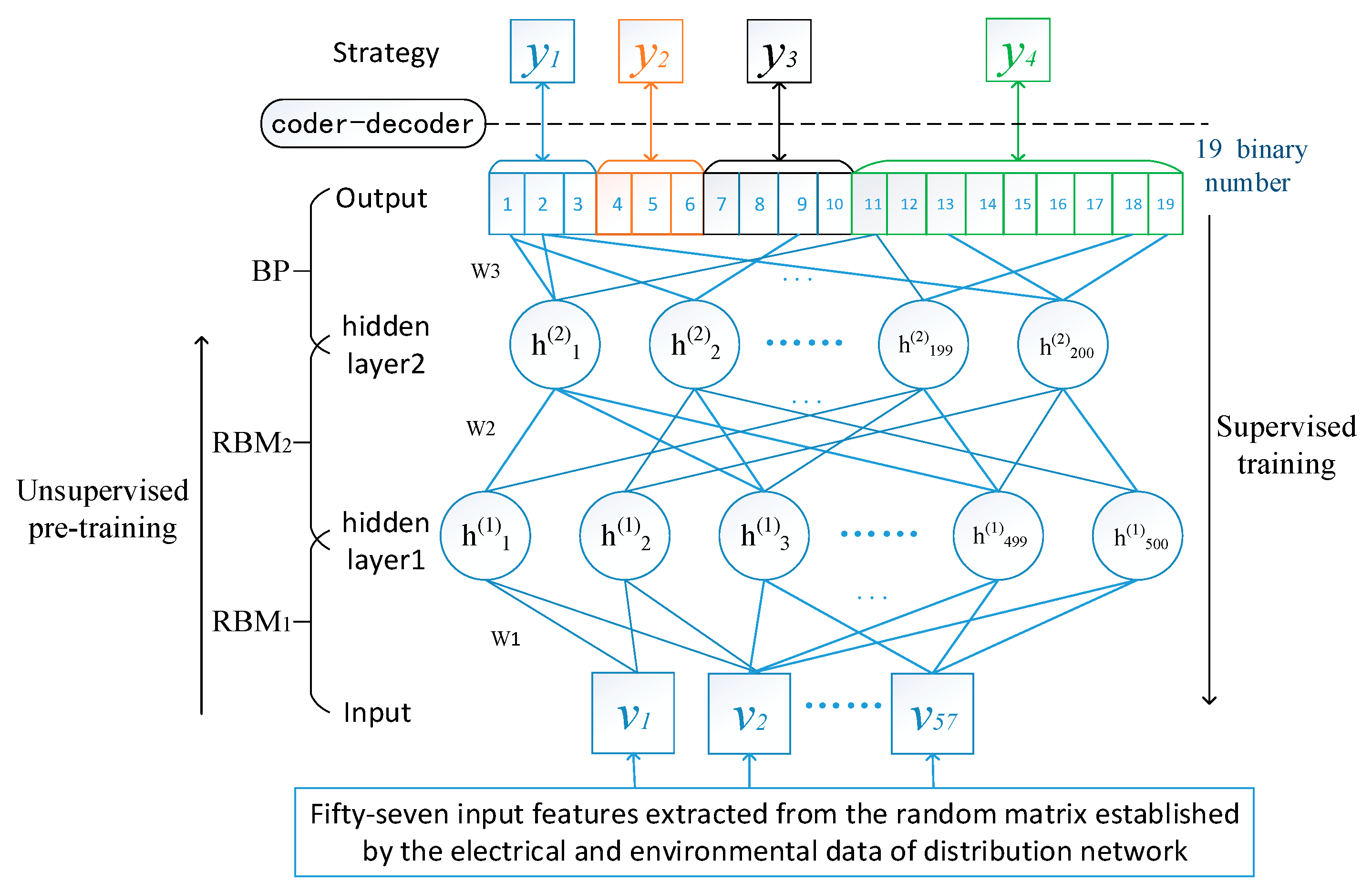
4.2. Control Solution Coder–Decoder

Since each hidden layer and output layer of DBN are binary variables, it is necessary to conduct binary coding for the historical reactive power optimization solution and take these variables as output labels to participate in the reverse supervision training. It is also necessary to decode the output binaries of the DBN model to the practical control solutions such as the tap changer position of the transformer and VAR output of each reactive power device when the offline training and online application are conducted.

The reactive power optimization devices used in the IEEE-37 benchmark model includes two fixed parallel capacitor groups C1 and C2, one OLTC (online tap changer) transformer with ±8 tap changers and one SVC with a capacitor of 300 kvar. The adjusted capacity of C1 and C2 are all 600 kvar (in units of 100 kvar); that is, 0–6. There are 2 × 8 + 1 = 17 tap positions for the transformer, and the SVC output is −300 to 300 kvar. These solutions correspond to 3, 3, 4, 9 bits of binary, and in total the 19-bit binary can be used to represent all reactive power optimization solutions. The control solution codec is actually the mapping of the actual policy and the 19-bit binary output unit of the DBN.

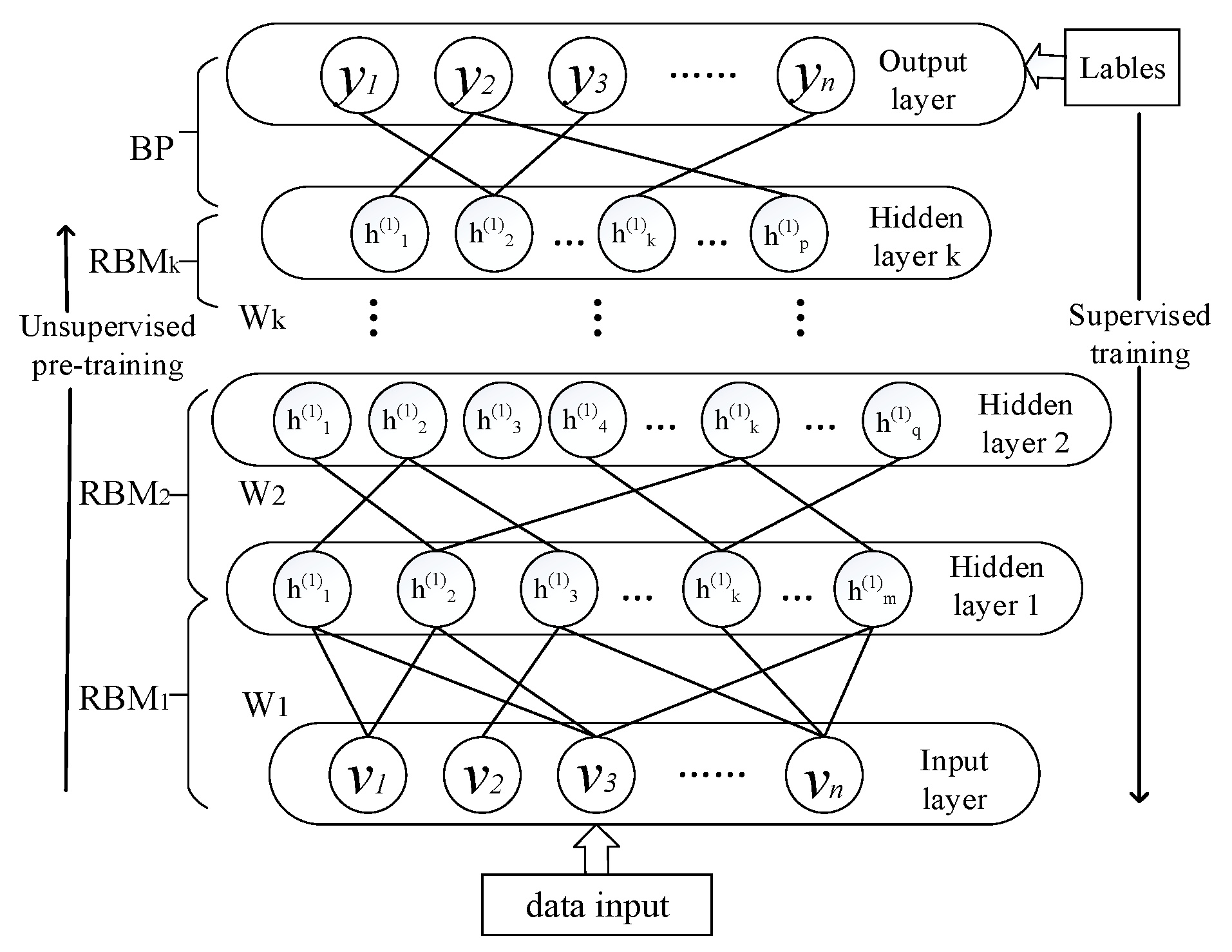
4.3. Modeling Processes

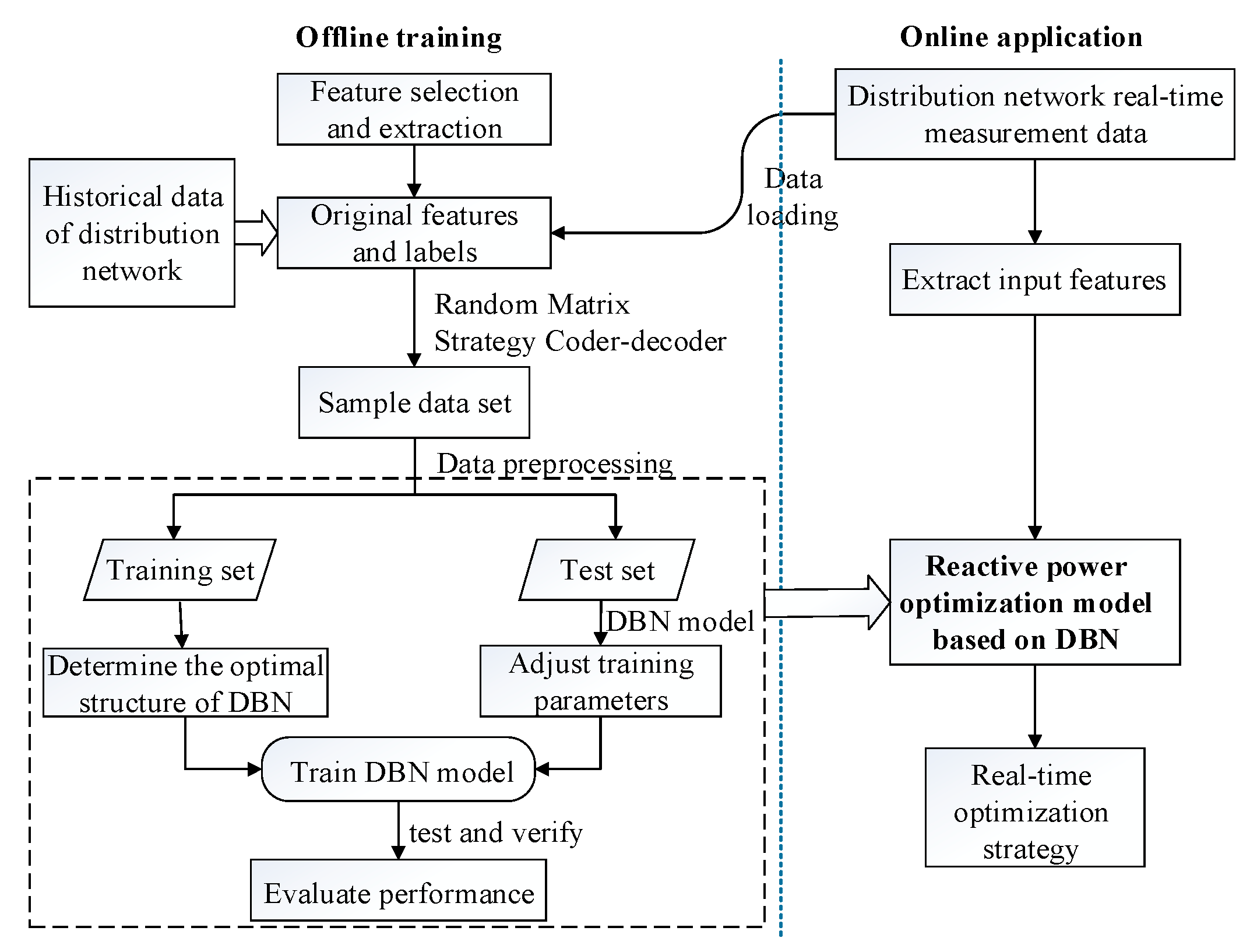
As illustrated in Figure 5, the construction processes of the reactive power optimization model of the distribution network based on DBN is composed of two stages: The offline training and online decision.

On the offline training stage, the main task is learning the corresponding relation between the features of distribution network and reactive power optimization solutions based on the historical data, which is similar to imitating and learning the judgment thinking and experience of the human-being dispatchers.

On the online application stage, it needs to extract high dimensional features quickly from a wide range of measurement data and then input them to the trained DBN model to find out the optimal reactive power control solutions.

Offline modeling processes are summarized as follows:

1.

Sample the historical data set and preprocessing.

Firstly, sample the original data and extract the features from the historical database of the distribution network and compose the feature data set with the random matrix. Meanwhile, code the corresponding reactive power optimization solution and construct the output tag set. In order to narrow the numerical difference of statistic features, the maximum and minimum normalization method expressed in Equation (11) is adopted to normalize the sample data to keep them all in the range of [0,1]. Then divide the normalized sample data set into a training set and test set.

$$C_{inew}=\frac{C_i-C_{\min }}{C_{\max }-C_{\min }},$$

(11)

where $C_i$ and $C_{inew}$ are the statistic features before and after normalization, respectively; and $C_{\max }$ and $C_{\min }$ are the maximum and minimum values of a certain statistic feature in the sample data set, respectively.

2.

Determine the optimal structure of DBN. Determine the number of hidden nodes and hidden layers of DBN network with the experimental method.

3.

Train the DBN model. The training stage includes three steps as follows:

(1)

The unsupervised pre-training. Take the 57 dimensions feature vector of reactive power optimization as inputs and train the RBM layer by layer from bottom-to-top.

(2)

The supervised parameter fine-tuning. Take the statistic features of the trained set as input and the coded reactive power optimization solutions as the corresponding labels. Fine-tune the network parameters from top-to-bottom until reaching the preset number of iterations.

(3)

Training parameter of DBN.

Input the statistic features of the test set into the trained DBN, and then decode the output layer binary data to obtain the actual adjustment solutions of test day. The control solution deviation ratio (SDR) expressed in Equation (12) is taken as the index to measure the performance of DBN training parameters. If the value of SDR is less than the set threshold value, the DBN training parameter will be reset until the SDR is basically stable below the threshold value.

$$er=0.25•(\frac{c_1}{r_1}+\frac{c_2}{r_2}+\frac{t}{r_3}+\frac{s}{r_4}),$$

(12)

where $c_1$, $c_2$, $t$ and $s$ represent the difference values between the input capacities of capacitor bank C1, C2, the transformer tap position, input capacity of SVC and their corresponding values obtained by conventional reactive power optimization solutions. $r_1,r_2,r_4$ represent the maximum capacities of SVC, and $r_3$ denotes the transformer tap position. It has been demonstrated that the smaller the value of $er$, the better the control effects of the control solutions obtained by the model.

4.

Evaluate the performance of the DBN model.

Apply the control solutions obtained by the DBN model to the test bed, and test whether the solutions can achieve the control effects in terms of network loss reducing and node voltage deviations.

5. Case Study

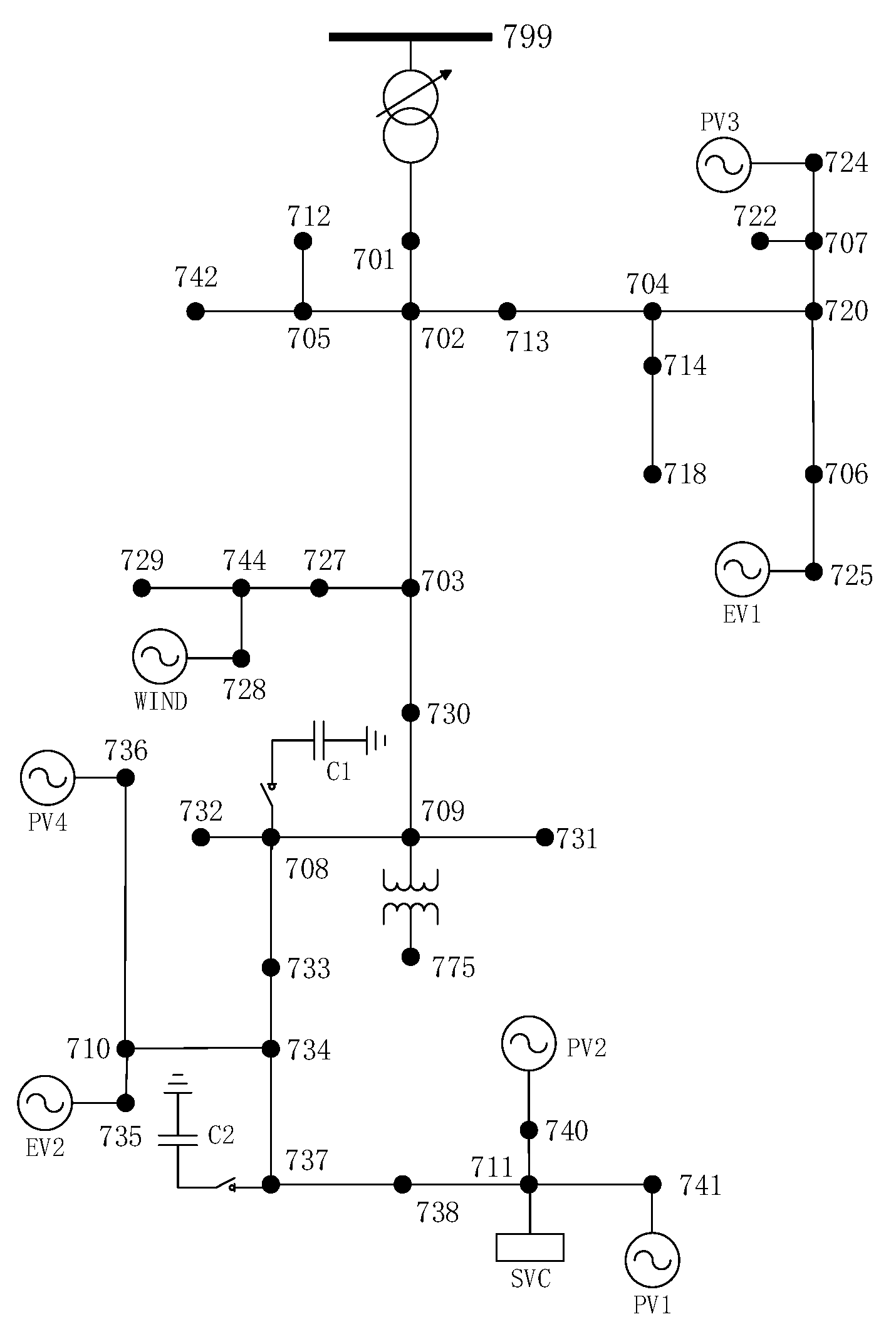
To demonstrate the effectiveness of the proposed method, the case studies were performed on the modified IEEE-37 nodes distribution network through the combined Matlab and OpendDSS software platform. The standard IEEE-37 nodes distribution network was modified moderately to consider stochastic loads and DGs (PV, WT and EV), and the topology and parameters of the modified distribution network are given in Appendix B in detail, see Figure A1 and

Table A2. Information of PV, EV and wind generator.

Connected Device	Position	Capacity
PV1	741	75 kVA
PV2	740	100 kVA
PV3	724	100 kVA
PV4	736	75 kVA
WT	728	300 kW
EV1	725	120 kW (Maximum power)
EV2	735	240 kW (Maximum power)

.

5.1. Conventional Reactive Power Optimization Method

In order to demonstrate the performance of the proposed scene-matching method and DBN model, the Particle Swarm Optimization (PSO) algorithm was selected as the conventional optimization method for comparison, and optimized control solutions in the historical database were also obtained by PSO. The objective of the conventional reactive power optimization in this paper is to minimize the active power loss while satisfying various constraints, and voltage deviation is also considered as small as possible by adding it as a penalty term to the objective function. Some key parameters of PSO were set as follows: The population size is 30, the maximum number of iterations is 50, the inertia factor ranges from 0.4 to 0.9 and the learning factor is 2.

5.2. Construction of Sample Data Set and Historical Database

The simulation model of the modified IEEE-37 nodes system is established based on the annual (8760 hours) historical load data and the actual environment data such as temperature and wind speed. The penetration of DGs including PV and WT is set to 10% (low penetration scenario). Because the access to the historical database of the distribution network is limited, the time-series simulation and calculation were performed in Matlab and OpenDSS software to obtain the original feature database and construct a high dimensional random matrix to extract features. Taking one year for example, it constitutes 8760 hours of historical samples. The hourly reactive power optimization solutions were obtained by PSO. These features and optimization solutions constitute the historical database for scene matching. Meanwhile, these data were processed as the input features and output labels of DBN. Then, the input and output were organized into a sample library to form a training set with 8760 valid historical samples.

5.3. Determining the Structures of DBN

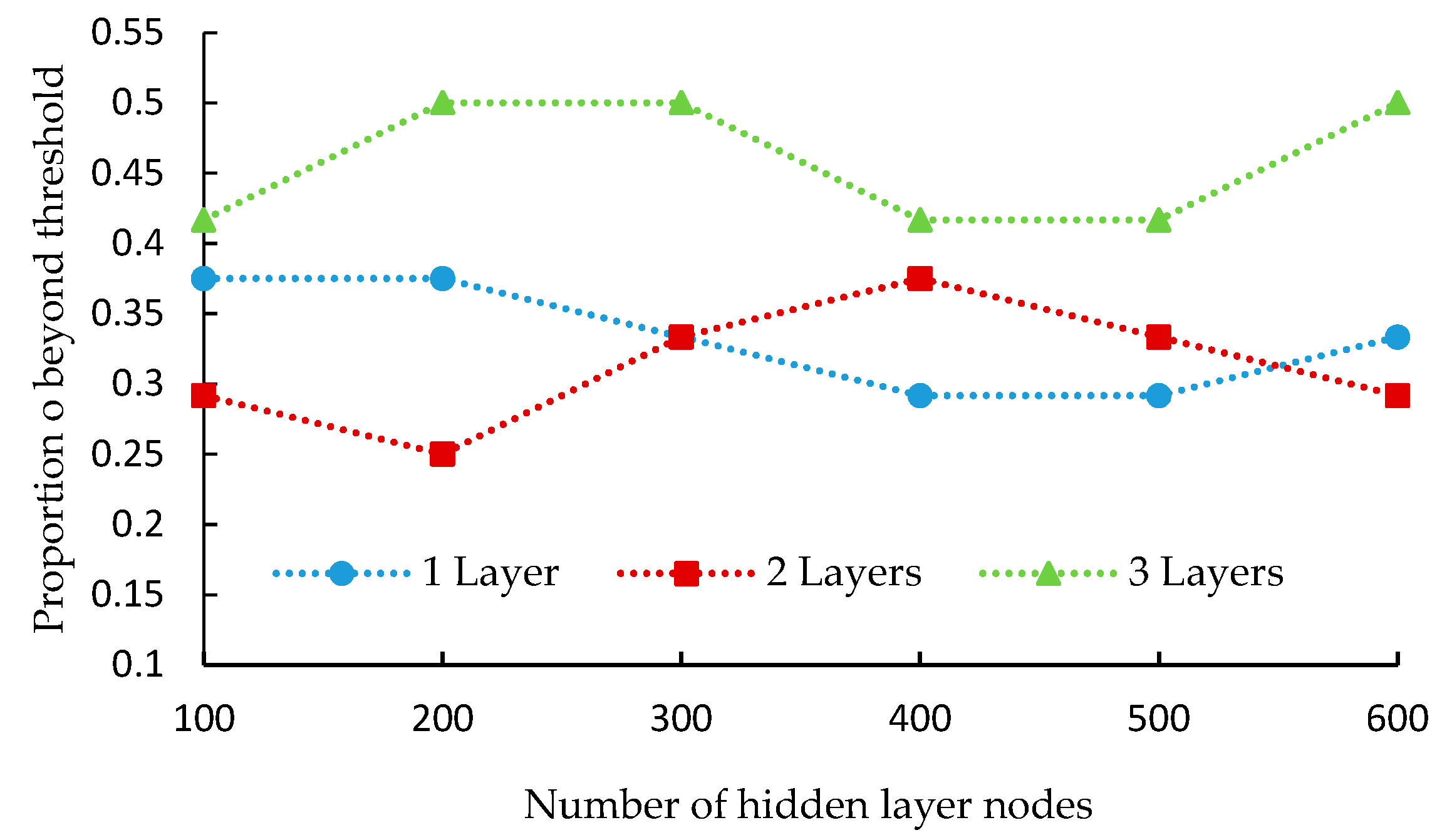
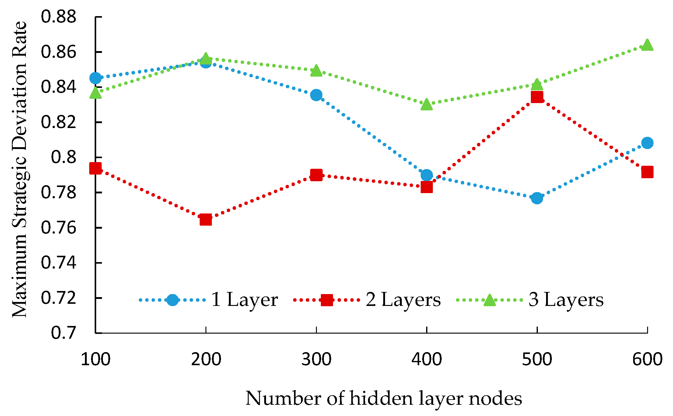
Too many hidden nodes will easily lead to over fitting and conversely will result in insufficient learning ability, thus determining the structures of DBN is a key issue for training DBN. However, no consensus has been reached about how to determine the optimal numbers of hidden layers and nodes. In this paper, we propose the following test method to determine the optimal numbers of hidden layers and nodes.

Firstly, set the network to contain only one hidden layer, and set the number of nodes to 100–600 by the step size of 100 to carry out DBN training, respectively. If the training effects satisfy the following optimal conditions, the corresponding node number is the optimal.

Optimal conditions: The maximum solution deviation rate Mer is the minimal; the above-threshold ratio Rer (the ratio of the hours that er > 0.5 to 24 hours) is the minimal. The definition of er is shown in Equation (12).

Secondly, fix the node number of the first layer, add a second hidden layer and set different node numbers to continue training to select the optimal node number of this layer.

And so on, until the variable values of the optimal condition will no longer decrease.

From the test results, it is found that there is a certain relationship between the training effects and the numbers of hidden layers and nodes, which are shown in Figure 6 and Figure 7.

From Figure 6 and Figure 7, we can see that the values of Mer and Rer are minimal when the hidden layer number is 2 and node number is 500 and 200. As the hidden layer increases to 3 layers, the values of Rer and Mer increases significantly. Therefore, the optimal structure of this DBN model is (57,500,200,19), as shown in Figure 8. Then, adjust the training parameters continuously to build the DBN model with er less than the threshold.

5.4. Results

In this section, we randomly select an actual typical day (24 h) in one year of the distribution network as the day to be optimized, utilize the above method to obtain the hourly features, and form a test data set with 24 under-optimization samples for RM scene-matching and DBN model effect comparison. The optimization results of this day can basically represent the statistical rules of many other days under optimization. These methods have also been applied to every day in a half of a year, and the statistical results of the performance comparison are given in Section 6.

5.4.1. Comparative Analysis

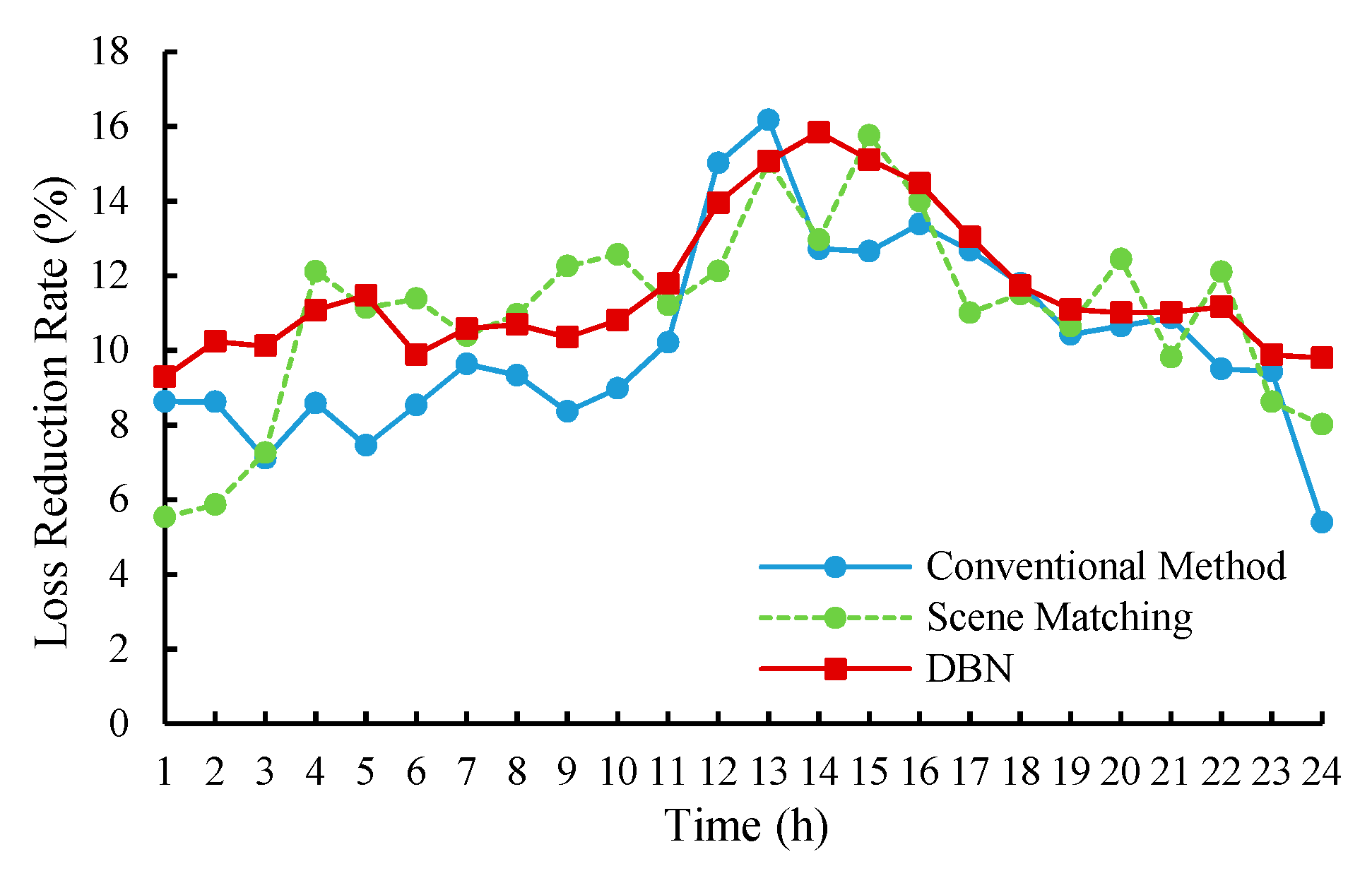
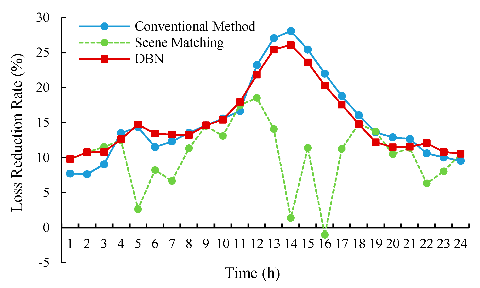
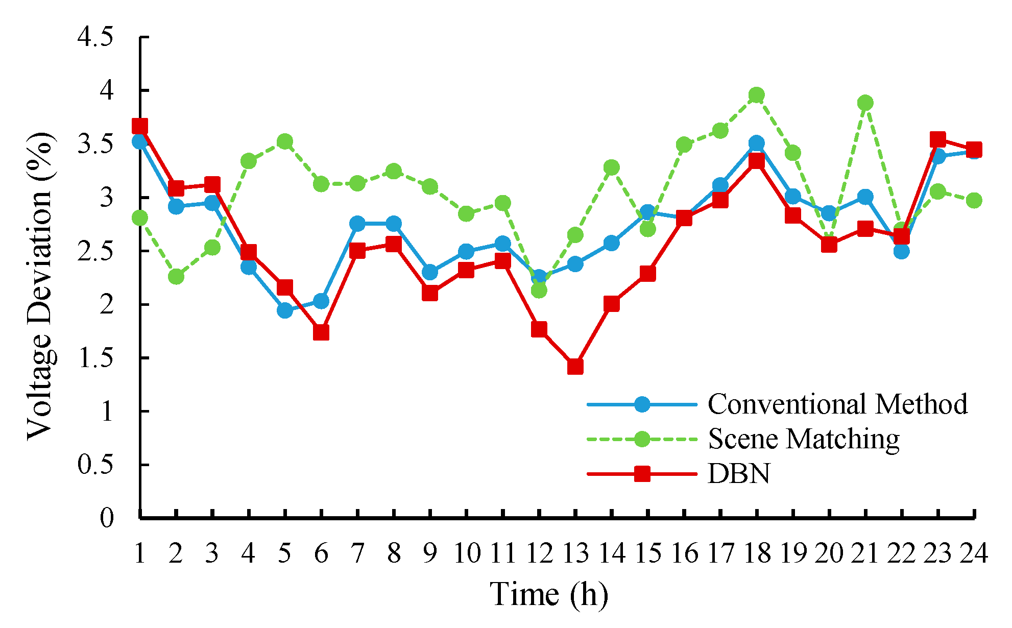
In this paper, the indices of loss reduction ratio and the voltage deviation are chosen to evaluate the reactive power optimization effects.

The active power loss reduction ratio is defined as

$$f_{LR}=\frac{P_0-\Delta P}{P_0}\times 100\%,$$

(13)

where, $P_0$ is the line loss of the distribution network without reactive power control at that time, and $\Delta P$ is the line loss after reactive power optimization at that time. The larger the loss reduction ratio is, the better the control performance is.

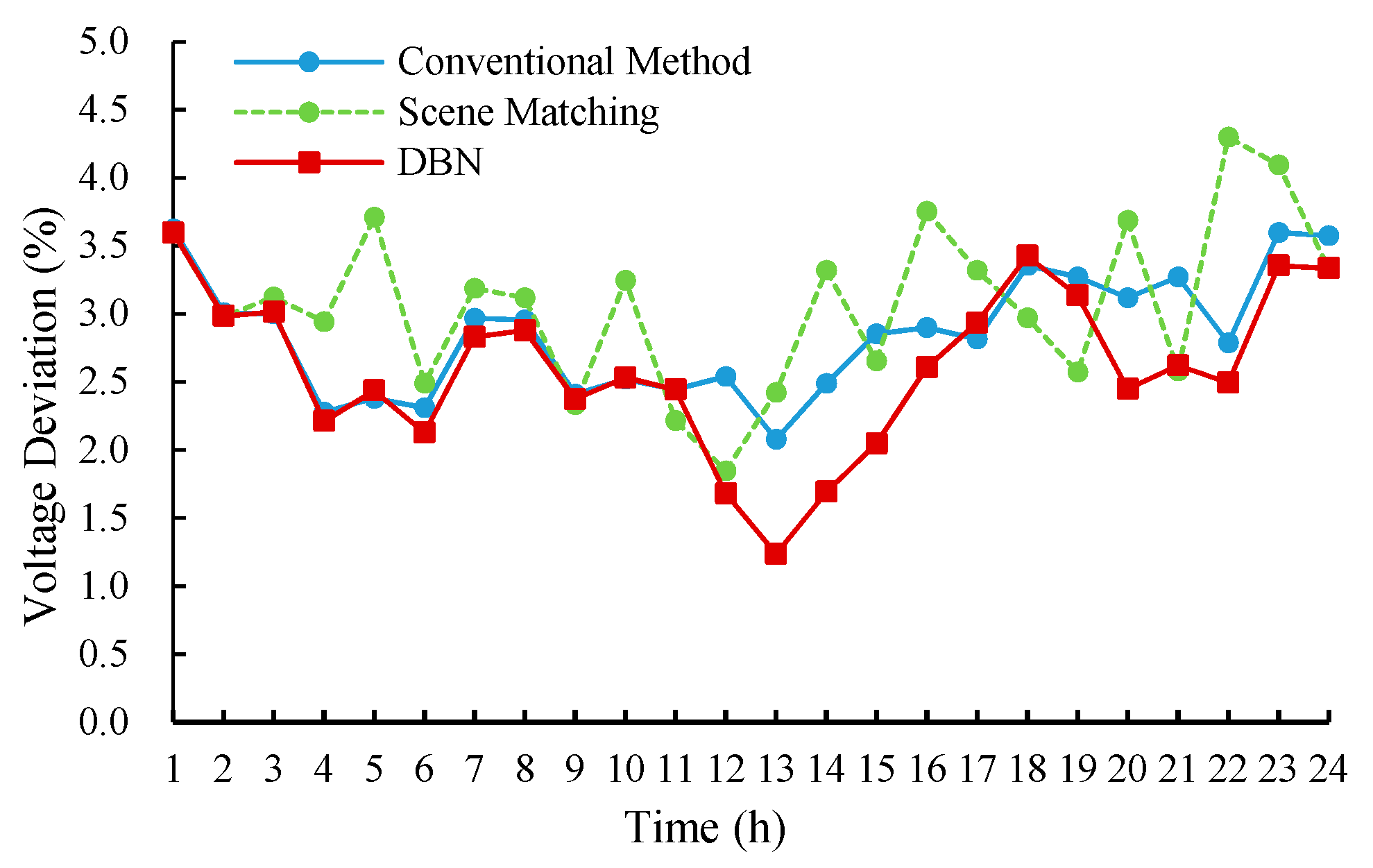
The system voltage deviation is defined as

$$\Delta U=\sqrt{\frac{1}{n}{\displaystyle \sum _{i=1}^n{(\frac{U_i-U_{iN}}{U_{iN}})}^2}}\times 100\%,$$

(14)

where $U_i$ is the actual voltage of i-th node, $U_{iN}$ denotes the nominal voltage and n is the node number. The less the voltage deviation is, the better the control performance is.

The results of loss reduction ratio and voltage deviation are shown in Figure 9 and Figure 10.

Comparing the scene-matching method with the conventional method, it can be seen that the loss reduction performance is similar for the two methods, and the voltage deviation index of the scene matching is slightly larger than the conventional method. Since the scene-matching method can only match similar scenarios in the historical database, it may not be applicable to the current system states.

Besides, the comparisons of the three methods show that the reactive power optimization model based on the DBN had a good performance in reducing power loss and decreasing the voltage deviation. Especially the performance in decreasing voltage deviation is even better than the conventional method.

The solutions obtained by the DBN model are effective and reasonable, which has learned the mapping relation between the operation state of the distribution network and the conventional optimization solutions. Under the guidance of the mined mapping rules, the DBN method can provide control solutions superior to the conventional method.

To further compare the three methods’ performance, we compared the data processing and optimizing time. Firstly, the scene-matching method in this paper for building history matching database need to calculate all kinds of random matrix features of one year’s history data (8760 samples), which costs 37.2 min. Meanwhile, DNB needs to conduct offline model training, and one year’s sample data is utilized, which costs about 26.1 min (DBN network parameter training only needs 0.332 s, and the rest of the time is for input feature data processing).

Once the historical database is built, and the DBN model is trained, we can use three methods to optimize the same scene online and measure the optimization run time of three methods, as shown in

Table 1. Run time of the three methods.

Method	Conventional Method	Scene Matching	DBN
Run Time	54.33 s	1.32 s	0.78 s

. All simulations were conducted under the test environment of MATLAB (Version R2016b) and OpenDss (Version 7.6.5.64), where the PC CPU was a Pentium(R)Dual-Core E5500 @2.80 GHz, and the RAM was 4 GB.

It can be seen that, compared with the conventional methods, the optimization of the two methods proposed in this paper is very fast, satisfying the requirements of the online reactive power optimization. It should be worth mentioning that the scene-matching and DBN-based approach do not depend on the distribution system model and parameters anymore, the only thing they use is the data generated by the distribution network; they are purely data-driven. And they can make the decisions more quickly than ever before because they do not need to perform the online optimizing calculations like conventional methods.

5.4.2. Under Higher DG Penetration

Most of the optimization methods based on being data-driven have limitations, such as they cannot properly analyze the scenes that have not occurred in the historical database, and they also show poor robustness. Meanwhile, due to the high penetration of grid-connected DGs, the node voltage and network loss of the distribution network are gradually increased [36]. Therefore, a more adaptive reactive power optimization method is needed to adjust the system operation states.

To verify the robustness of the methods proposed in this paper, the penetration of DGs (PV and WT) is increased from 10% to 20%. The results of the loss reduction ratio and voltage deviation are shown in Figure 11 and Figure 12.

The results show that the DBN model trained and obtained under the low DG penetration is still available for the reactive power optimization demands in the higher DG penetration scenario. Besides, the performance of loss reducing of the DBN method is similar to the conventional method, and the voltage deviation index of the DBN method is better than the conventional method. However, for the scene-matching method, the performances for loss-reducing and voltage deviation are deteriorated, especially during the noon period when the DG output power increases significantly. That is because it is hard to find out the matching scenarios from the historical database, and the control effects become worse as the matching degree goes down.

Meanwhile, as an innovative data-driven reactive power optimization method, the DBN-based method can learn the nonlinear complicated relationships between system statistic features and reactive power optimization control solutions, which breaks through the bottleneck of the scene-matching methods. It can still provide appropriate reactive power control solutions directly and quickly, even for some new unknown scenes that have not appeared in the historical database. From this perspective, the DBN-based method possesses excellent adaptability and robustness, which can provide a feasible solution to the problem of reactive power optimization of the large-scale grid-connections of DGs.

6. Discussion

In order to exclude the influence of stochastic factors as far as possible, we still take 8760 h of the above year as the historical data, and select another half year (4,344 under-optimization moments) as the test data. That is to say, to expend the tests and verifications in Section 5 from one day (24 h) to half of a year (4344 h). In this section, the conventional method is used as the comparison benchmark, and we mainly compare the differences between the methods proposed in this paper and the conventional method. Therefore, two comparative indicators, network loss acceptability and voltage deviation acceptability are defined as follows:

$$L_W=\frac{\Delta P_D-\Delta P_{CN}}{\Delta P_{CN}}\times 100\%,$$

(15)

where $L_W$ is the network loss acceptability at a certain time, $\Delta P_D$ is the network loss at that time when the system adopts reactive power optimization solution by methods in this paper (RM scene-matching and DBN model), and $\Delta P_{CN}$ is the network loss at that time when the system adopts conventional PSO reactive power optimization.

$$U_W=\Delta U_D-\Delta U_{CN},$$

(16)

where U_W is the voltage deviation acceptability of system at a certain time, $\Delta U_D$ is the system voltage deviation at that time when the system adopts method proposed in this paper, and $\Delta U_{CN}$ is the system voltage deviation at that time when the system adopts the conventional PSO method.

According to the definition of voltage deviation acceptability U_W and network loss acceptability L_W, the smaller their values are, the better the optimization performance is. Specifically, when the U_W or L_W is less than 0, it means that the voltage deviation or the network loss is smaller than the conventional one, that is, the optimization effect is better.

Considering that there are a large number of test samples (4344) to be optimized, in order to compare the optimization effect of the methods more intuitively and comprehensively, we choose the distribution probability of these two indicators in 4344 samples as the statistical indicator of the optimization effect. We define the Excellence-Ratio and Qualified-Ratio as follows:

$$R_e=\frac{N_1}{4344}\times 100\%,\hspace{1em}\hspace{1em}where L_w<0,U_w<0,$$

(17)

$$R_q=\frac{N_2}{4344}\times 100\%,\hspace{1em}\hspace{1em}where L_w<5\%,U_w<1\%.$$

(18)

Among them, the Excellence-Ratio Re is expressed as the proportion of the excellent performance cases among 4344 test moments in half a year, where N₁ is the number of test samples when the Network Loss Acceptability L_W is less than 0 and the Voltage Deviation Acceptability U_W is also less than 0 at the same time, indicating that the optimization effect at this time is comprehensively better than the optimization effect of conventional methods.

The Qualified-Ratio Rq is expressed the proportion of the qualified performance cases among 4344 test moments, where N₂ is the number of test samples when the L_W is less than 5% and the U_W is less than 1%, indicating that the optimization effect at this time is either better than the conventional optimization effect, or slightly lower than the conventional effect but close to it. It is in the acceptable range, and it can meet the current reactive power optimization requirements of the distribution network.

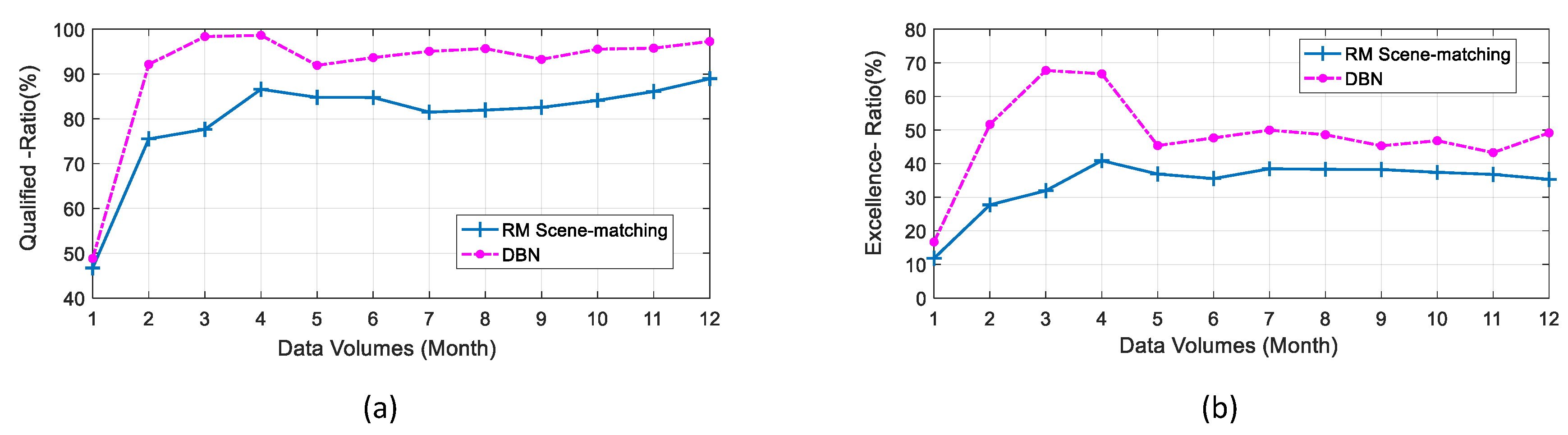
6.1. The Influence of Historical Data Volumes on Optimization Results

In order to further study the influence of each methods on the reactive power optimization effect under different historical data volumes, this section composes 12 data sets with different data volumes from 8760 historical data samples of a year, and increases the data volumes by one month as a unit to form data sets containing historical samples of 1, 2, 3,…, 12 months, respectively, for scene matching and DBN model training. Another half of one year (4344 h) samples of the distribution system are also selected as the test scene to be optimized. The optimization results of various methods under different data volumes are shown in

Table 2. Comparison of reactive power optimization effect of the two methods under different data volumes.

Data Volumes (Month)	Scene-Matching Method		DBN-Based Method
	Qualified-Ratio Rq	Excellence-Ratio Re	Qualified-Ratio Rq	Excellence-Ratio Re
1	46.71%	11.83%	48.83%	16.69%
2	75.51%	27.74%	92.15%	51.70%
3	77.65%	31.95%	98.37%	67.73%
4	86.60%	40.88%	98.64%	66.74%
5	84.78%	36.90%	91.94%	49.37%
6	84.76%	35.54%	93.67%	47.65%
7	81.49%	38.47%	95.07%	49.98%
8	81.95%	38.31%	95.67%	48.60%
9	82.55%	38.24%	93.28%	47.30%
10	84.12%	37.41%	95.56%	46.82%
11	86.10%	36.79%	95.76%	47.28%
12	89.13%	35.34%	97.28%	49.15%

and Figure 13.

It can be seen from the above charts that both the Qualified-Ratio Rq and the Excellence-Ratio Re are increased with the data volume. After four or six months, these changes stop, and Rq and Re start to fluctuate randomly in a certain range.

According to the comprehensive analysis of two methods, when the amount of historical data is small, the performances of both the scene matching and DBN-based methods are poor. However, with the increase of historical data volume, DBN only needs just more than two months of training samples to ensure the reactive power optimization effect of the model, and the Rq and the Re are very high. The scene matching requires up to four months data to ensure a stable Rq between 80%–90%, and both the Re and Rq are lower than the DBN method. It indicated that the overall reactive power optimization performance of DBN is relatively higher, and the DBN model has significant advantages beyond other methods even in the case of fewer training historical data.

6.2. The Influence of Different DG Penetration on Optimization Results

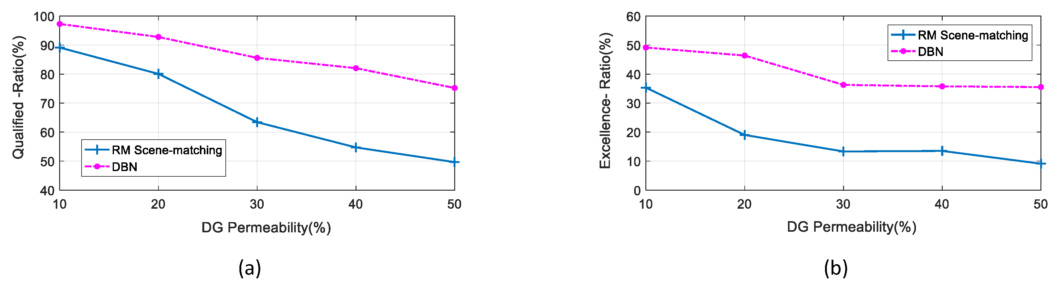
In order to further study the influence of different DG penetration scenarios on the reactive power optimization of each method, this section will increase the DG penetration. The original DG penetration is 10%, and there are five different test scenarios with the DG penetration of the simulation model are set to 10%, 20%, 30%, 40% and 50%.

We selected the data sample for another half year (4344 h) under the five penetration scenario as the test set to be optimized. For RM scene matching, the original 10% low-penetration historical database is still used to match the high penetration scenarios. For DNB optimization, 10% low-penetration training samples were still used to optimize the higher penetration scenario, and the results are shown in

Table 3. Comparison of reactive power optimization effect of the two methods under different DG penetration.

Penetration	Scene-Matching Method		DBN-Based Method
	Qualified-Ratio Rq	Excellence-Ratio Re	Qualified-Ratio Rq	Excellence-Ratio Re
10%	89.13%	35.34%	97.28%	49.15%
20%	80.06%	19.01%	92.79%	46.39%
30%	63.42%	13.33%	85.59%	36.28%
40%	54.72%	13.51%	82.04%	35.77%
50%	49.65%	9.12%	75.21%	35.52%

and Figure 14.

Table 3 shows that with the increase in DG penetration, the Qualified-Ratio Rq and the Excellence-Ratio Re of each method decline to different degrees, and the changing trend is consistent.

Under the scenarios with different penetration, we can see that the solutions generated by the DBN model have better reactive power optimization effect than the scene-matching method, and the Rq and the Re tend to decrease more slowly with the increase of penetration.

The scene-matching method is greatly affected by penetration changes, especially when the penetration exceeds 20%, the optimization effect decreases and the performance gets worse. This is because with the increase of the DG penetration, it becomes harder to find out the most similar and most matching scene from the original historical database.

When the penetration is less than 40%, the Rq and the Re of the DBN-based method are less affected by the high penetration scene of DG, and the effects are still acceptable. The Rq can stay above 80%, the Re remain above 35% and the Rq is only slightly worse when the penetration reaches 50%. This result also indicates that the DBN-based model trained and established under the condition of only 10% penetration is still feasible to the high-penetration scenarios of 20% to 40%, furtherly verifying the robustness and generalization of the proposed DBN-based approach.

7. Conclusions

To take advantages of the Big Data of the huge historical operation data, this paper proposed two data-driven methods for the reactive power optimization of the active distribution network, the feature-based scene-matching method and DBN-based method. The comprehensive case studies were conducted on the modified IEEE-37 active distribution network, and the reactive power optimization effects of the proposed approaches were investigated and compared with the conventional method. The influences of the historical data volume and the adaptability under higher DG penetrations were also discussed. We can derive the following conclusions:

(1)

Combining the random matrix theory with the time-series method, this paper suggested two ways to construct the random matrix and extracted 57 statistical features to represent the operating characteristics of the distribution network. These features can be utilized in the scene-matching method and DBN training for reactive power optimization effectively.

(2)

The data-driven scene-matching method and the DBN-based deep learning method of reactive power optimization are proposed in this paper, as both of them can achieve a similar performance to the conventional method or even better with more than four months historical operation data. The merits of these two data-driven methods are that they do not depend on the distribution system models and parameters anymore and are purely data-driven. The only thing they used were the data generated by the distribution network. They can make the on-line decisions more quickly and satisfy the online optimization requirements of the distribution network operation.

(3)

The DBN-based deep learning method always possesses better performance than the scene-matching approach, even under the unknown higher DG penetration cases, verifying the adaptability, robustness and generalization ability. This paper provided a new and innovative way for the application of Big Data and Artificial Intelligence in reactive power optimization of the distribution network.