An Investigation into the Effects of Weak Interfaces on Fracture Height Containment in Hydraulic Fracturing

Abstract

Hydraulic fracturing is an effective method for developing unconventional reservoirs. The fracture height is a critical geometric parameter for fracturing design but will be limited by a weak interface. Fracture containment occurs when fracture propagation terminates at layer interfaces that are weaker than the surrounding rock. It always occurs in multilayer formation. Therefore, the mechanism of fracture height containment guides fracture height control in hydraulic fracturing. In order to study the fracture containment mechanism, this paper first calculates the propagation behaviour of the fracture in 3D under the influence of a weak interface through a block discrete element method and analyzes the geometric characteristics of the fracture after it meets the weak interface. Then, the induced stress of the hydraulic fracture on the weak interface is calculated by fracture mechanics theory, and the mechanism of blunting at the fracture tip is explained. Then, two kinds of interface slippage that can lead to blunting of the fracture tip are discussed. Based on the behavior of shear slippage at the interface, a control method for multilayer fracturing in thin sand-mud interbed and pay zone fracturing in shale is proposed. The results show that the fracture height is still limited by the weak interface in the formation without the difference of in-situ stress and rock properties. Interface slippage is the main factor impeding fracture propagation. Fracture height containment can be adjusted and controlled by changing the angle between the hydraulic fracture, the interface, and the stress state to strengthen and stiffen the interface. This study has a certain guiding significance for fracture height control in the design of hydraulic fracturing of shale or thin sand-mud interbed reservoirs.

1. Introduction

Hydraulic fracture containment occurs when fracture propagation terminates at layer interfaces that are weaker than the surrounding rock [1]. As shown in Figure 1, the fluid-driven fracture (green region) is initialized and propagates around the well in the pay zone at the early stage. Then, the fracture encounters interfaces (red lines). The fracture cannot penetrate the interface vertically; the height (H) of the fracture is contained, and the fracture can only propagate laterally. Therefore, the fluid-driven fracture is contained in the pay zone. In some cases, such as extraction of shale gas and CO₂ sequestration, fractures must be contained mainly in the pay zone because fractures breaking out into overlying or underlying formations in the water-bearing zone can lead to irreparable water damage to the formation [2,3], similar to Figure 1. On the contrary, in other cases, such as hydraulic fracture in thin sand-mud interbed, fractures must pass through the mud layer to connect isolated hydrocarbon-bearing layers to penetrate through the fracture into the well [4,5]. This is called trans-layer fracturing, shown in Figure 2. The former case requires fracture containment to keep the fracture in the pay zone, whereas the latter case requires no fracture containment to penetrate layers. Therefore, the mechanism of fracture containment is significant for hydraulic fracturing design for different reservoirs.

Over the past half-century of development of hydraulic fracturing technology, many field tests, laboratory experiments, and numerical simulations were conducted on fracture containment. The mechanism for fracture containment is divided into three categories: stress contrast of adjacent layers, rock property contrast between layers, and weak interfaces. At the end of the 20th century, the effect of stress contrast became the main reason for fracture containment. The stress contrast means the differences in in-situ stress between adjacent layers. This is commonly the case in conventional sandstone reservoirs targeted for hydraulic fracture stimulation, which have lower minimum in-situ stress compared with the adjacent shale layers. For example, the stress of the pay zone is lower than the overlying or underlying zone in Figure 1 [4]. This is supported by fracture mechanics theory [6,7,8] and laboratory and field experiments [9,10,11,12]. The literature [13,14,15] also shows that fracture height containment in shale caused by stress differences is common. Therefore, the most obvious explanation for the observed containment of fractures in reservoirs is stress difference between the reservoir and the adjacent cap rock. It is also accepted that properties of different layers have an influence on fracture height. These two reasons are always studied together using analytical [16] or numerical [2,14] methods.

In recent years, researchers have focused on the effects of a weak interface. An experimental study of hydraulic fracture containment was carried out with an analogue layered reservoir constructed from transparent materials by Xing et al. [3,17]. There are four types of fracture geometries: containment, height growth, T-shaped growth, and the combination of height and T-shaped growth with different interface fracture toughness. More numerical investigations into fracture containment related to a weak interface were conducted with different methods. Based on a finite element method, a 3D fluid-solid coupling model was established with Abaqus code by Wang et al. [18] to simulate hydraulic fracturing problems. Their results indicate that when the shear strength of the interface is lower than a critical value, obvious slippage between the barrier layer and the pay zone occurs, and the fracture tip becomes blunted. Tang [19] developed the displacement discontinuity method (DDM) to investigate slippage of weak horizontal interfaces and understand the effects of the slippage on fracture height growth. Weng et al. [4] and Chuprakov and Prioul [1] developed the FracT model to examine shear slippage along the bedding interface. This model considered strength and frictional properties and effective vertical stress at the frictional and cohesive interface. The results of the FracT model show that slippage of the fracture tip leads to fracture blunting, which hinders the propagation of fracture height growth.

The above investigations into interfaces indicate that weak interfaces play an important role in fracture containment. Previous studies have shown that the interface hinders the propagation of fractures. However, the question of why the interface hinders the propagation and behavior of fractures has not been clearly answered. To understand the role of a weak interface in fracture containment, the mechanisms of fracture tip blunting and interface slippage were investigated by a simplified model of real rocks in this study. First, fracture height containment was studied by block discrete element to investigate fracture propagation without stress contrast and distinct layer properties. The result leads to the conclusion that the interface is one reason for fracture containment, besides the stress state and rock properties. Fracture containment still exists with the same stress and rock properties. Then, the stress field on the interface is calculated by fracture mechanics with the same stress state and rock properties. Finally, the slippage forms at the interface, including shear failure and discontinuous displacement, are discussed, along with measures for fracture containment for the purpose of multilayer or pay zone fracturing.

Our main contributions are as follows. This paper explains that fracture-tip blunting is the key factor that hinders fracture propagation. The shape of the fracture tip at the interface is described, and the fracture tip is explained as being due to interface slippage. Considering interface slippage, the control parameters for fracturing under different reservoir conditions are proposed.

The rest of the paper proceeds as follows. The method and numerical model are introduced in Section 2. The propagation behavior of the fracture in 3D under the influence of a weak interface is calculated with the block discrete element method and the geometric characteristics of the fracture after it meets the weak interface are analyzed in Section 3. The induced shear stress and normal stress of the hydraulic fracture on the interface are calculated in Section 4.1, and two slippage models are introduced in Section 4.2. Finally, the control method of multilayer fracturing in thin sand-mud interbed and pay zone fracturing in shale is proposed.

2. Method and Model

2.1. Block Discrete Element Method

2.1.1. Constitutive Model of Joints

The thickness of the joint is far lower than the scale of its plane, so its deformation characteristics are described by the stress-displacement relationship. The constitutive relationship of the structural plane mainly examines the relationship between the stress of the structural plane and its normal and tangential deformation. There are two stresses on the structure surface, normal stress σ and shear stress τ, and two corresponding displacements, normal displacement δ_n and tangential displacement δ_s. The stress displacement relationship matrix is expressed as [13,20,21,22]:

$$\left\{\begin{array}{c}\sigma \\ \tau \end{array}\right\}=\left\{\begin{array}{cc}{K}_n& K_{ns}\\ K_{sn}& K_s\end{array}\right\}\left\{\begin{array}{c}{\delta }_n\\ {\delta }_s\end{array}\right\}$$

(1)

where $K_n=\frac{\partial \sigma }{\partial {\delta }_n}$ is the normal stiffness coefficient and represents the effect of normal displacement on normal stress; $K_s=\frac{\partial \tau }{\partial {\delta }_s}$ is the shear stiffness coefficient and represents the effect of shear displacement on shear stress; $K_{ns}=\frac{\partial \sigma }{\partial {\delta }_s}$ is the dilation stiffness coefficient and represents the effect of shear displacement on normal stress; and $K_{sn}=\frac{\partial \tau }{\partial {\delta }_n}$ represents the effect of normal displacement on shear stress.

The Goodman element is adopted in this calculation, i.e., K_sn and K_ns are set as 0, and K_n and K_s are used to describe the normal deformation and tangential deformation of the structural surface, respectively. The Goodman element is one of the most commonly used interface elements to describe the interface characteristics of discontinuous medium such as faults or joints [23], and the Goodman elements method is employed in some numerical software such as RFPA [24] or 3DEC [25]. The details about the Goodman element method can be found in [26].

The Mohr–Coulomb (M–C) equation for shear strength of structure plane is

$$\tau =c+f\sigma$$

(2)

where f = tan (φ), and c, φ are cohesive strength and friction angle of structural plane, respectively.

2.1.2. Contact Friction Joint Model

The contact friction joint model and Coulomb slip model are used in this calculation. Assuming that the structural plane has no thickness, the rock masses on both sides are in close contact. The contact elements cover the surface of the rock on both sides. In the boundary of the two contacts, one surface is referred to as the target surface and the other as the contact surface. The role of the structural plane is achieved by contact pair interaction, and the contact friction behavior between them obeys the M–C law [27].

It is assumed that the normal stress increment F_n (compression is positive), and the shear vector increment F_s between blocks are proportional to the normal displacement u_n and the tangential displacement increment u_s in the elastic stage. The contact stiffness of the normal and tangential springs is k_n and k_s, respectively. Assuming that there is no tension in the joint and Coulomb’s law is satisfied, the relationship can be expressed as [21,22]:

$$F_n=k_n{u}_n,\hspace{1em}while\hspace{1em}{u}_n\le 0$$

(3)

$$F_n=0,\hspace{1em}while\hspace{1em}{u}_n>0$$

(4)

$$F_s=k_s{u}_s,\hspace{1em}while \left|F_{cs}\right|\le f\left|F_{cn}\right|+cL$$

(5)

$$F_s=sign\left(u_s^{\prime }\right)\left(f\left|F_{cn}\right|+cL\right),\hspace{1em}while \left|F_{cs}\right|>f\left|F_{cn}\right|+cL$$

(6)

where F_n and F_s are the normal and tangential components of contact force F_c, respectively; k_n and k_s are the normal and tangential stiffness of joints, respectively; u_n and u_s are the normal and tangential relative displacements of joints, respectively; F and c are the friction coefficient and cohesive force of joint material, respectively; and L is the length of the contact surface.

2.1.3. Fluid Flow in Fracture

It is assumed that the fracture surfaces are impermeable, and fluid flows only between the fracture surfaces. The flow of fluid in the fracture satisfies the cube law [28]. The modified cube law is

$$q=-\frac{u_h^3\rho g}{12\mu }{\nabla }_h=-K_h{\nabla }_h$$

(7)

where q is the fluid flow rate per fracture width, u_h is the equivalent hydraulic aperture, ρ is the density of the fluid, $\mu$ is fluid dynamic viscosity, $\nabla$h is the hydraulic gradient, and K_h is hydraulic conductivity.

In the hydro-mechanical coupling of fractures, the influence of mechanical deformation on fracture permeability is mainly manifested as a change in fracture aperture. In the elastic stage, the fracture aperture is expressed as an equation related to the effective stress [25]:

$$u_{he}=u_{h0}+f_1\frac{\Delta {\sigma }_n^{\prime }}{k_n}$$

(8)

In the plastic stage, considering the expansion caused by joint slip, the fracture opening can be expressed as [25]:

$$u_{hp}=u_{h0}+f_1\frac{\Delta {\sigma }_n^{\prime }}{k_n}+f_1{u}_{hs}$$

(9)

where u_h0 is the initial fracture aperture, $\Delta {\sigma }_n^{\prime }$ is effective stress, and f₁ is a coefficient for the influence of stiffness, set as 1 in this study.

2.1.4. Motion Equation of Blocks

The deformation of blocks is nonnegligible. The blocks are divided into tetrahedral units. The vertices of a tetrahedral element are called grid difference points. The motion equation is established at each node as follows [21,22]:

$$u_i^{\prime }=\frac{{\displaystyle {\int }_s{\sigma }_{ij}{n}_{j}ds}+F_i}{m}+g_i$$

(10)

where s is the outside surface, m is the mass on the grid point, g_i is the acceleration of gravity, and F_i is the result of an external force applied to a node. n_j is the unit normal vector pointing to the outside. The integral represents the sum of forces on the surface.

The node force ∑F_i is 0 in the balance state. Otherwise, there is an acceleration of node according to Newton’s second law.

$${u_i^{\prime }}^{\left(t+\Delta t/2\right)}={u_i^{\prime }}^{\left(t-\Delta t/2\right)}+{\displaystyle \sum F_i^{\left(t\right)}}\frac{\Delta t}{m}$$

(11)

For every time step, strain, and rotation are related to displacement. Their forms are as follows:

$${\epsilon }_{ij}^{\prime }=\frac{1}{2}\left(u_{i,j}^{\prime }+u_{j,i}^{\prime }\right)$$

(12)

$${\theta }_{ij}^{\prime }=\frac{1}{2}\left(u_{i,j}^{\prime }-u_{j,i}^{\prime }\right)$$

(13)

An incremental method is applied in the calculation. It is not limited to small strain problems. Therefore, the constitution model of deformation blocks takes an incremental form. The equation is as follows

$$\Delta {\sigma }_{ij}^e=\lambda \Delta {\epsilon }_v{\delta }_{ij}+2\mu \Delta {\epsilon }_{ij}$$

(14)

where λ and μ are Lamé coefficients and δ_ij is the Kronecker function.

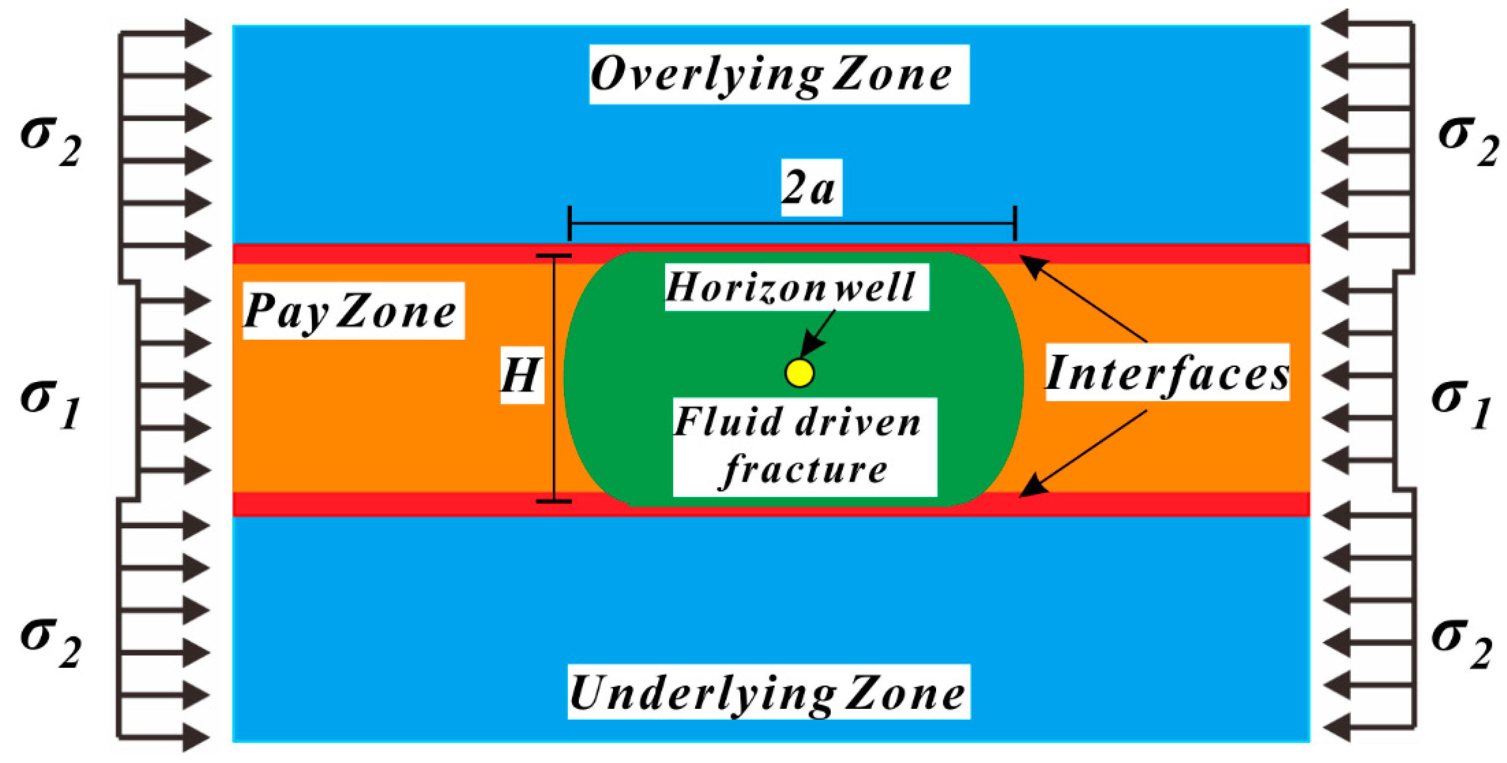
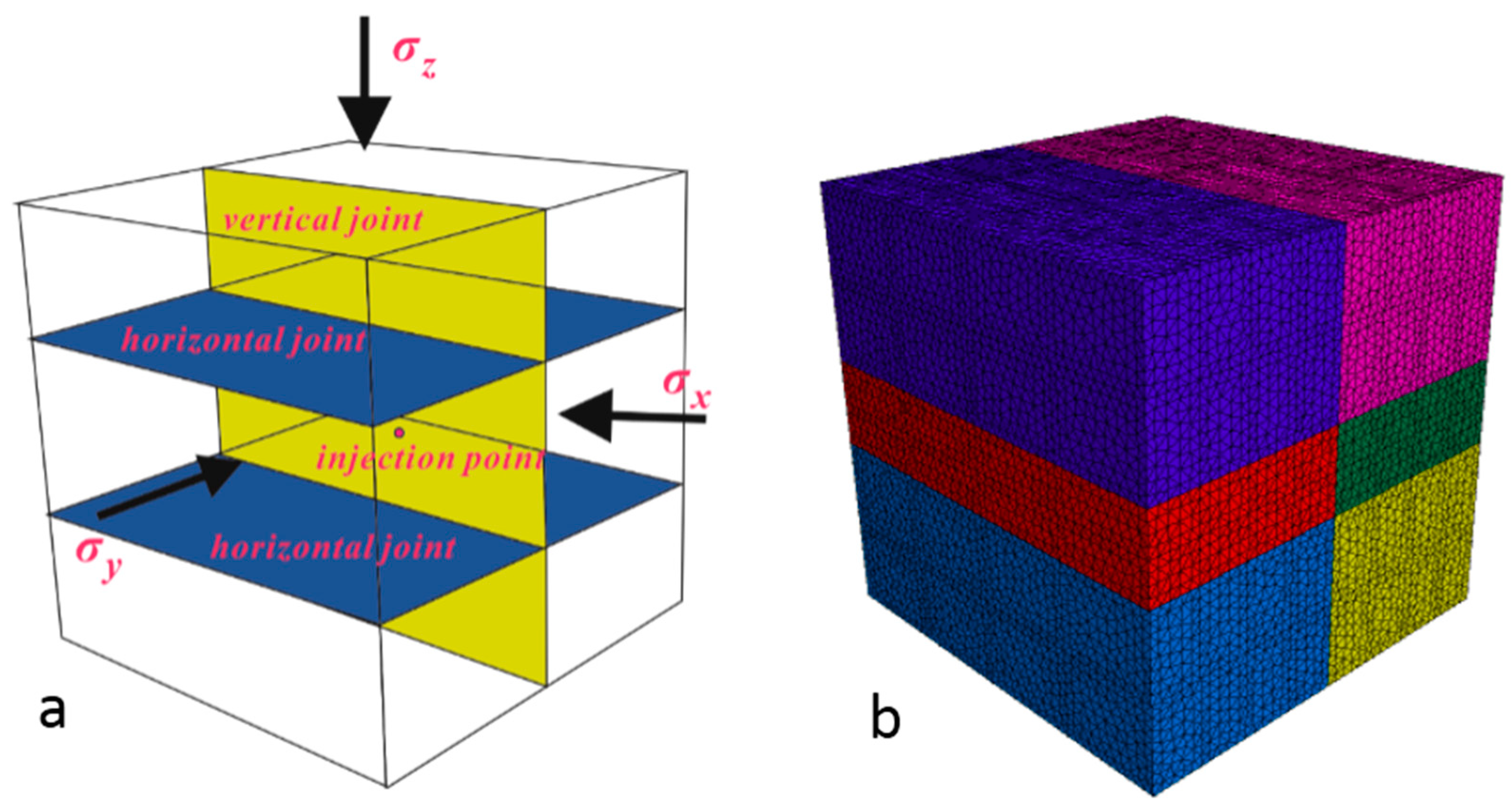
2.2. Numerical Model Description

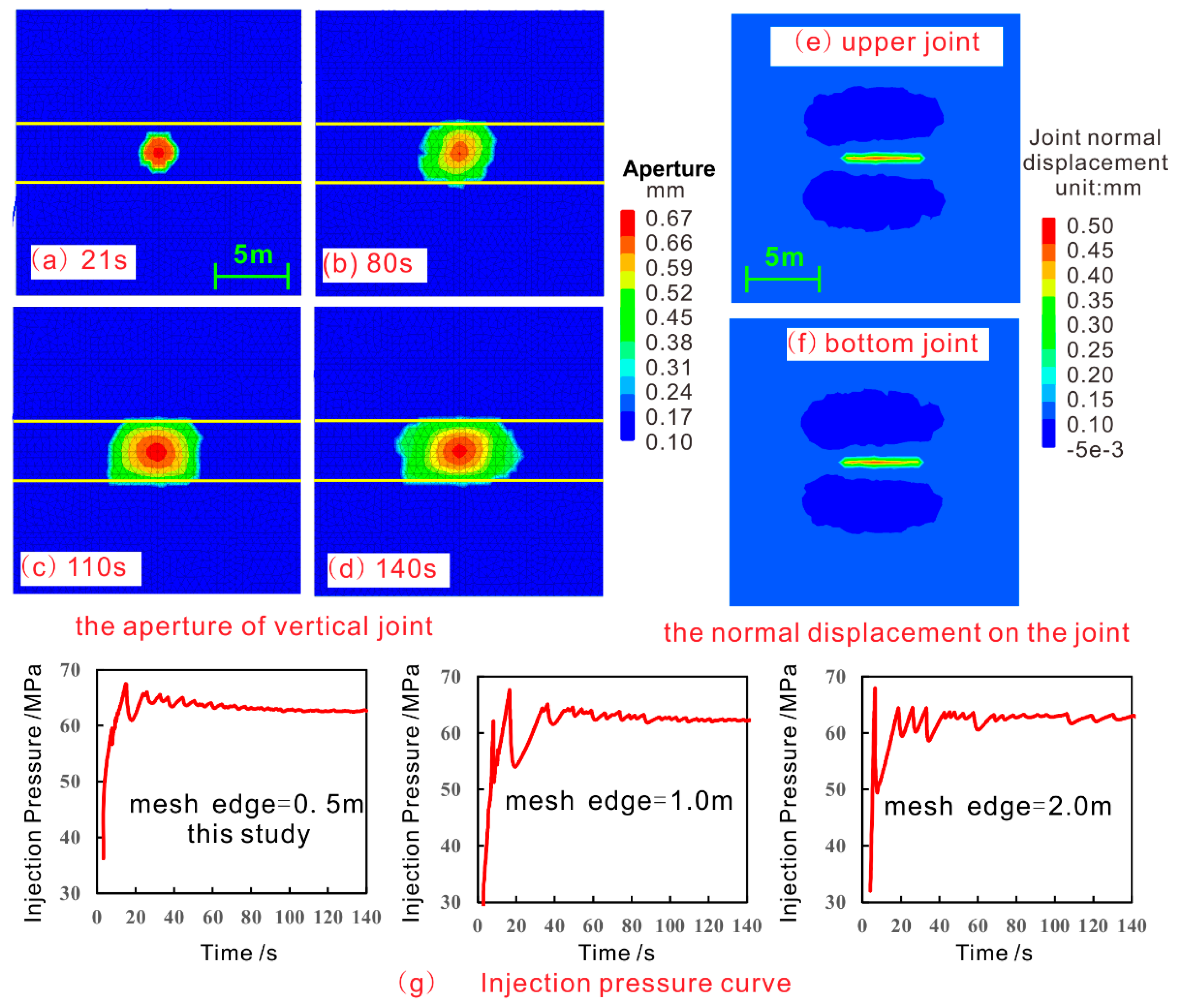
Based on block discrete element theory, the propagation behavior of hydraulic fractures in rock mass with cemented joints is simulated by the following model. The model, shown in Figure 3, includes two horizontal joints and one vertical joint and can simulate the behavior of fracture crossing and fracture containment. The intersection angle between the vertical and horizontal joints is 90°. In order to eliminate the interference of in-situ stress and rock properties, the stress and properties of the three parts are the same. The distance between the centers of the two horizontal joints is 4 m. The model is a 20 m cube. The two horizontal joints are 2 m away from the injection point. The edge of the grid is 0.5. The values of parameters for simulation are listed in detail in

Table 1. Values of parameters for simulation [25].

Parameter	Value	Parameter	Value
Elastic modulus	20 GPa	Fluid viscosity	0.0015 Pa.s
Poisson’s ratio	0.25	Fluid density	1000 kg/m3
Density of rock (ρ)	2600 kg/m3	Depth (h)	3000 m
Joint friction	20°	Injection rate	0.01 m3/s
Joint cohesion	0 MPa	Initial vertical stress	76.518 MPa

. The rock properties in our simulation are based on shale, and the fluid is based on water. The parameters are the same as those in the help document of three-dimensional distinct element method code (3DEC) software [29]. The maximum principal stress is equal to the vertical stress. The minimum principal stress is 61.21 MPa. It is 0.8 times the vertical stress.

The numerical modeling is carried out with 3DEC, in which the material is modeled as a discontinuous medium that consists of two types of elements, blocks and discontinuities. The validation of numerical simulation for hydraulic fracture was conducted by Zhang and Dontsov [13] and Gil et al. [20]. Their results, calculated by 3DEC, determine the availability of the block discrete method in hydraulic fracturing. Therefore, fracture height containment was studied with 3DEC software in this study. Besides, the model in this study only considers fluid flow in fractures. The flow in formation is not considered for the low permeability of real shale.

The purpose of this model is to study fracture height containment without stress contrast and distinct layer properties. With the model built above, the geometries of fluid-driven fractures were obtained with uniform stress and rock properties. The results are shown in the next section.

3. Results

The geometries of fluid-driven fractures were obtained with the same stress and rock properties. That means that there is no difference in the in-situ stress and rock properties. The results are shown in Figure 4. As mentioned above, the injection point was set on the vertical joint, leading to fracture propagation on that joint. The geometries of fractures are displayed by the apertures of joints. The highest value is in red, and the initial value is in blue (it may actually be 0, but for numerical calculation, a minimal value of 1 × 10⁻⁴ m was set). The injection pressure was also monitored over time, displayed in the figure as purple curves. The two intersection lines of vertical and horizontal joints are plotted with two white lines.

The curve in Figure 4g shows injection pressure from 0 s to 140 s. As shown in the figure, the pressure increases and decreases rapidly in the initial period. The fracture is initialized when the injection pressure reaches 65.0 MPa. Then, there is a fluctuation period after the fracture opens. Finally, the pressure tends to be smooth and steady at 63 MPa. Injection pressure increases rapidly before the fracture initiation. After fracture initiation, the flow will be directed into the new fracture. This results in a drop in pressure within the fracture. The continuous injection of fluid continues to squeeze the fracture, and the pressure gradually increases. In the early stage of fracturing, the fracture volume is small, and the ratio of new extended fracture volume to existing fracture volume is large. In this case, the flow of fluid to the new fracture will lead to an obvious pressure drop. On the contrary, when the existing fracture volume is large, the newly generated fracture volume has little influence on the pressure inside the fracture. Therefore, the injection pressure fluctuates greatly in the initial fracturing period. As injection time increases, fracture volume increases. As a result, the pressure fluctuations in the later stages of fracturing gradually decrease. The fluctuation occurs with a constant rate because of the volume ratio of the new open fractures to the existing fractures.

It is mentioned above that the fluctuation of pressure curve is correlated with the spatial volume changes caused by the new fracture. In the numerical calculation, the volume change caused by fracture of rock mass is related to the grid size, so the mesh dependency analysis is carried out. The tetrahedral mesh is adopted in this paper. The size of the mesh is determined by the edge. Therefore, the edge is selected as 0.5 m, 1.0 m, and 2.0 m for examining mesh dependency. The injection pressure curves of the three cases are shown in Figure 4g. According to the figure, the pressure fluctuation of the curve is affected by mesh size. With the increase of mesh size, the fluctuation of pressure curve is more obvious, and the duration of fluctuation is longer. But they still satisfy the rules mentioned above. The fluctuations are greatest in the early stage of fracturing and decrease with time. As for the influence of mesh size, it can be concluded that mesh size will affect the fluctuation of curves, but the fluctuation rule of the pressure curve is still consistent.

The overall trend of the injection pressure curve is as follows: The pressure first rises and then begins to decrease when the initiation pressure is reached and then gradually stabilizes. This trend is consistent with the trends of a laboratory experiment [30], a simulation [31], and a field test [32]. This means the simulation results are suitable for the research. Compared with the previous results, more details of the pressure fluctuations in fracture propagation are demonstrated in our results.

For the fracture geometries, the fracture only propagates between two intersection lines in Figure 4a and meet an intersection in Figure 4b. In Figure 4a, the fracture is seen to propagate freely in the vertical joint without any hindrance. Then, the fluid-driven fracture meets the intersections between the vertical and horizontal joints. The fracture cannot penetrate the intersections but only propagates to the lateral sides (left and right in Figure 4a–d) between the two horizontal joints. The lateral length of the fracture increases but the height remains constant (Figure 4c,d). The fracture height is contained by the two horizontal joints. The fluid-driven fracture does not penetrate the intersections in Figure 4a–d. This means that the fracture does not propagate beyond the two lines. The normal displacement of horizontal joints at 140 s, the time of Figure 4d, is plotted in Figure 4e,f. As shown in the figures, there is only displacement near the intersections and no fracture propagating in horizontal joints. In a word, the fracture only propagates between the two intersection lines. The fracture height is contained in this simulation.

As mentioned above, there are three main reasons for fracture containment: stress contrast, property difference, and weak interface. The above results are based on the condition that the same stress state and rock properties exist among upper, middle, and bottom parts of the model. Therefore, the effects of stress contrast and property difference can be eliminated. Then, the weak interface is the only one that affects height containment in this study.

The effect of a weak interface on fracture height containment was investigated in this study. As shown in Figure 4e,f, the displacements of the two horizontal joints were similar, and the model was symmetrical. Therefore, the stress on them was also similar. Then, we chose one of the horizontal joints. To understand the mechanics of the interface in fracture containment, the shear and normal stress on horizontal joints were plotted in Figure 5a,b. The horizontal line in the center is the intersection with the vertical joint. The shear stress is plotted in Figure 5a. It can be seen that there are two zones of increased shear stress on both sides of the intersecting line in the center of the graph. The stress in those two zones is larger than the others. The normal stress is plotted in Figure 5b. The reduction zone of normal stress is distributed along the intersecting line in the center of the graph, and there are two zones of increased normal stress on both sides of the intersection, consistent with Figure 4e,f. In Figure 4e,f, there are two zones with negative values on both sides of the intersection, indicating compression. Therefore, the normal stress increases in those two zones. In sum, along and near the intersection line, the shear stress increases, and the normal stress reduces when the fracture in the vertical joint meets the intersection. For a surface, if shear stress increases and normal stress decreases, the probability of relative slippage on the surface increases. Once slippage occurs, normal displacement of the joint is no longer smooth.

The aperture curves along the vertical line passing through the center point of the vertical joint for four steps over time are plotted in Figure 5c. There is distinct discontinuous displacement at −2 m, where the interface is. The result indicates that the fluid-driven fracture was hindered by the interface and the fracture tip became blunted. Based on Figure 5c, the geometries of fractures in every step are plotted in Figure 5d. It obviously shows the discontinuous displacement at the interface, indicating slippage. Therefore, one reason for fracture height containment is fracture tip blunting caused by interface slippage.

The conclusion above is that interface slippage is one reason for fracture containment, along with stress state and rock properties. The fracture containment still exists with the same stress state and rock properties. The formation of same stress state and rock properties means the same layer. In other words, fracture containment also exists in one layer that has cemented or natural fractures. The mechanism of interface slippage is critical for fracture containment. Why does normal stress decrease and shear stress increase? The stress state on the surface is the key factor for slippage. Therefore, the stress state and discontinuous slippage are discussed in the next section.

4. Discussion and Analysis

Fracture tip blunting caused by interface slippage is shown in Figure 6. The shape of the fracture is consistent with Figure 5d. The upper zone opened with pressure first. However, slippage occurred because of the weakness of the interface, which led to discontinuous displacement between the upper and bottom zones. The aperture of the fracture in the bottom is very small, which is set for numerical calculation; the actual aperture is not so wide, as shown in Figure 6; this just gives a better picture of the interface slippage. In this figure, the discontinuous displacement caused by slippage is clearly shown. Therefore, the behavior of the interface is key for this study. To understand the mechanism, the stress state of the interface is needed.

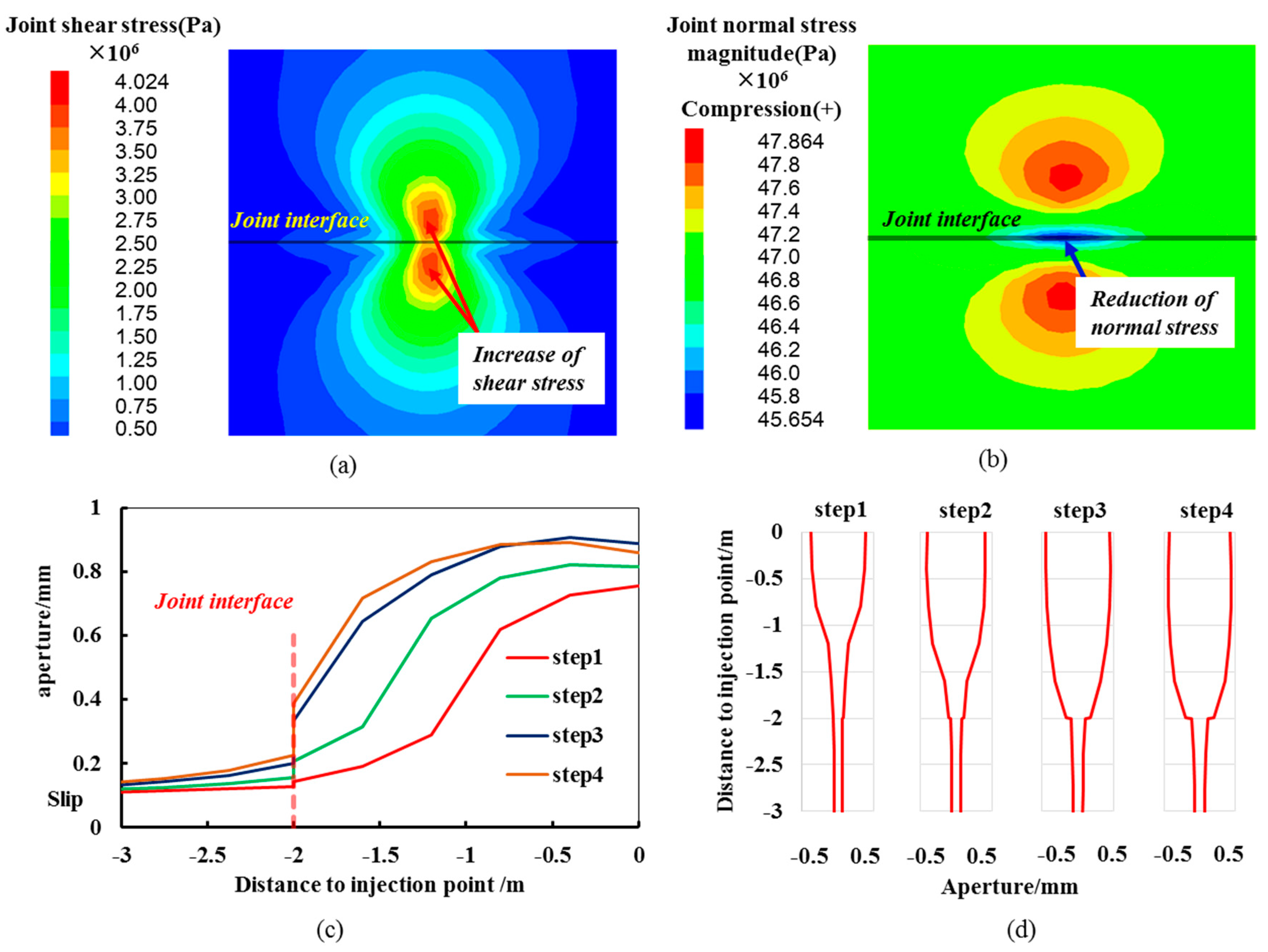
4.1. Stress State of the Interface

The stress state of the interface is important for slippage. Although it can be obtained by a numerical method, the analytical method is also important. The analytical solution based on fracture mechanics is discussed below.

As shown in Figure 7, a model in which the fluid-driven fracture approaches but does not reach the joint intersection with fluid pressure in the fracture is established according to model I. The distance between the fracture tip and the intersection is set as d, and the half-length of the fracture is a. Assuming that the joints are cemented before opening, the rocks can be regarded as a continuum. With that assumption, the stress state around the fracture can be express as follows [33]:

$${\sigma }_{xx}=\mathrm{Re}{Z}_{\mathrm{I}}\left(z\right)-y\mathrm{Im}{Z}_{\mathrm{I}}^{\prime }\left(z\right)+A$$

(15)

$${\sigma }_{yy}=\mathrm{Re}{Z}_{\mathrm{I}}\left(z\right)+y\mathrm{Im}{Z}_{\mathrm{I}}^{\prime }\left(z\right)-A$$

(16)

$${\tau }_{xy}=-y\mathrm{Re}{Z}_{\mathrm{I}}^{\prime }\left(z\right)$$

(17)

where Z_I is the Westergaard stress function. The detail is shown in Appendix A and Appendix B. The symbol A is a coefficient related to the boundary condition.

Polar coordinates with the fracture endpoint as the origin are introduced as $\zeta =r{e}^{i\theta }$ (Figure 8). This is also called a polar coordinate system of the fracture front. Then,

$$z=a+r_0{e}^{i\theta }=a+\zeta$$

(18)

According to Figure 8, the distance from the fracture tip to the joint surface is d, and the distance from a certain point on the joint surface to the x-axis is y; then, d, a, y, and r satisfy the following relationship:

$$r=\frac{d}{\cos \theta }$$

(19)

$$d=ka$$

(20)

$$y=d\tan \theta =a\cdot k\tan \theta$$

(21)

It can be ascertained that the interference stress field of fracture tip (r < < a) is

$${\sigma }_{xx}={\sigma }_{\mathrm{I}}^e\left(\sqrt{\frac{\cos \theta }{2k}}\cdot \cos \frac{\theta }{2}\left(1-\sin \frac{\theta }{2}\cdot \sin \frac{3}{2}\theta \right)\right)$$

(22)

$${\tau }_{xy}={\sigma }_{\mathrm{I}}^e\left(\sqrt{\frac{\cos \theta }{2k}}\cdot \cos \frac{\theta }{2}\sin \frac{\theta }{2}\cos \frac{3}{2}\theta \right)$$

(23)

The above two formulas can be expressed as ${\sigma }_{ij}={\sigma }_{\mathrm{I}}^e\cdot f_{ij}\left(\theta ,k\right)$, where f_i is

$$f_{xx}\left(\theta ,k\right)=\sqrt{\frac{\cos \theta }{2k}}\cdot \cos \frac{\theta }{2}\left(1-\sin \frac{\theta }{2}\cdot \sin \frac{3}{2}\theta \right)$$

(24)

$$f_{xy}\left(\theta ,k\right)=\sqrt{\frac{\cos \theta }{2k}}\cdot \cos \frac{\theta }{2}\sin \frac{\theta }{2}\cos \frac{3}{2}\theta$$

(25)

See Appendix A for the specific derivation process. Equations (24) and (25) are functions independent of a, but related to the relation coefficient k between d and a. Once the k value is determined, the distribution of f_ij function in the joint (y-direction) can be obtained; f_ij represents the coefficient of induced stress and is related to θ, but the distance along the y direction and angle θ are nonlinear. To plot f_ij along the joint parallel to the y-axis, the polar coordinates are transformed into rectangular coordinates. Then, $y=(k\tan \theta )\cdot a$ with $(k\tan \theta )\cdot a$ as the abscissa; the relationship between the induced stress coefficients and the distance on the y-axis can be plotted. The f_ij function under k = 0.01, k = 0.02, and k = 0.03 is calculated, and the results are shown in Figure 9.

It can be seen from the figure that the hydraulic fracture causes positive induced stress in joints, which means that it is tensile stress. Moreover, it is mainly distributed in the fracture tip and mainly in the range of 0.05 a. The closer to the center, the higher the value. Considering the original formation stress more fully, the induced stress can offset the original compressive stress and reduce the normal stress on joints. Similarly, shear stress caused in the range of 0.05 a is large. This indicates that the hydraulic fracture will cause a reduction of normal stress and an increase of shear stress on joints. This result is consistent with Figure 5.

The orthogonal joint conditions are deduced above. Based on a similar method, the stress states on nonorthogonal joint planes can also be deduced. Similar to Figure 8, the coordinate positions of nonorthogonal joints are shown in Figure 10, where the angle between the oblique joint (orange line segment) and the x-axis is δ, and the distance between a point on the joint and the intersection is L. Then, the relationship between L, r, and d can be expressed as

$$\frac{r}{\sin (\pi -\delta )}=\frac{L}{\sin \theta }=\frac{d}{\sin (\pi -\theta -(\pi -\delta ))}$$

(26)

$$r=\frac{d\sin (\pi -\delta )}{\sin (\delta -\theta )}$$

(27)

$$L=\frac{d\sin \theta }{\sin (\delta -\theta )}$$

(28)

Similarly, take out the coefficient f_ij (θ, k) as follows:

$$f_{xx}\left(\theta ,k\right)=\sqrt{\frac{\sin (\delta -\theta )}{2k\sin \delta }}\cdot \cos \frac{\theta }{2}\left(1-\sin \frac{\theta }{2}\cdot \sin \frac{3}{2}\theta \right)$$

(29)

$$f_{yy}\left(\theta ,k\right)=\sqrt{\frac{\sin (\delta -\theta )}{2k\sin \delta }}\cdot \cos \frac{\theta }{2}\left(1+\sin \frac{\theta }{2}\cdot \sin \frac{3}{2}\theta \right)$$

(30)

$$f_{xy}\left(\theta ,k\right)=\sqrt{\frac{\sin (\delta -\theta )}{2k\sin \delta }}\cdot \cos \frac{\theta }{2}\sin \frac{\theta }{2}\cos \frac{3}{2}\theta$$

(31)

The stresses in the x- and y-directions are converted to the oblique joint, and the normal stress and shear stress on the oblique joint are obtained as

$${\sigma }_n={\sigma }_{xx}{\sin }^2\theta +{\sigma }_{yy}{\cos }^2\theta +{\tau }_{xy}2\sin \theta \cos \theta$$

(32)

$${\tau }_s=\sqrt{{{\sigma }_{xx}}^2+{{\sigma }_{yy}}^2-{{\sigma }_n}^2}$$

(33)

$${\sigma }_n={\sigma }_{\mathrm{I}}^e\left(f_{xx}\left(\theta ,k\right){\sin }^2\theta +f_{yy}\left(\theta ,k\right){\cos }^2\theta +f_{xy}\left(\theta ,k\right)\sin 2\theta \right)={\sigma }_{\mathrm{I}}^e{f}_n\left(\theta ,k\right)$$

(34)

$${\tau }_s={\sigma }_{\mathrm{I}}^e\sqrt{f_{xx}{\left(\theta ,k\right)}^2+f_{yy}{\left(\theta ,k\right)}^2-f_n{\left(\theta ,k\right)}^2}={\sigma }_{\mathrm{I}}^e{f}_s\left(\theta ,k\right)$$

(35)

The dimensionless coefficient of induced stress on oblique joints is extracted as

$$f_n\left(\theta ,k\right)=f_{xx}\left(\theta ,k\right){\sin }^2\theta +f_{yy}\left(\theta ,k\right){\cos }^2\theta +f_{xy}\left(\theta ,k\right)\sin 2\theta$$

(36)

$$f_s\left(\theta ,k\right)=\sqrt{f_{xx}{\left(\theta ,k\right)}^2+f_{yy}{\left(\theta ,k\right)}^2-f_n{\left(\theta ,k\right)}^2}$$

(37)

At δ = π/2, $\sqrt{\frac{\sin (\delta -\theta )}{2k\sin \delta }}=\sqrt{\frac{\sin (\pi /2-\theta )}{2k\sin \left(\pi /2\right)}}=\sqrt{\frac{\cos \theta }{2k}}$; thus, Equations (29) and (31) degenerate to (24) and (25), indicating that the results of this inference are consistent; fτ and fn at δ = π/2 are plotted in Figure 11a, which is consistent with Figure 5. See Appendix B for the specific derivation process

Shear slippage on the interface is a key factor for fracture containment. Shear stress is considered the main factor for slippage. Therefore, we should focus on the change of shear stress on the interface. The induced shear stress coefficients with different angles δ are plotted in Figure 11b. The target range is less than 0.5 a. The relationship between the coefficient of shear stress at distance 0.1 a and angle δ is plotted in Figure 11c. As shown in the figure, the coefficient decreases at a range of 15°–30° and increases at a range of 30°–90°; the lowest value is at 30°, and the highest is at 90°. Angle δ describes the angle between the fluid-driven fracture and the joint, which are perpendicular at δ = 90°. This indicates that, when the fracture is orthogonal to the joint, the shear stress on the weak surface is highest, and the probability of slippage is highest. In this situation, fractures are always contained in the pay zone by interfaces. On the contrary, the shear stress on the weak surface and the probability of slippage are the lowest when δ = 30°. In this situation, fractures tend to penetrate the interlayer and connect other layers. To sum up, angle δ should be selected according the form of the reservoir in hydraulic fracturing. The intersection angle can be controlled by the fracture angle in formation. The fracture angle can be adjusted by the perforating angle and stress field. The stress field can be modified by artificial intervention. The artificial intervention of stress is also being studied by researchers. Interface slippage is related to shear stress. As it is one of the main factors of containment, higher shear stress is more prone to fracture containment. The lowest value is at 30° and the highest is at 90°. Therefore, when fractures need to propagate in the pay zone (fracture containment), they should be perpendicular to the interface (90°). When fractures need to connect multilayers, they should be at a 30° angle to the interfaces.

4.2. Slippage Forms on Interface

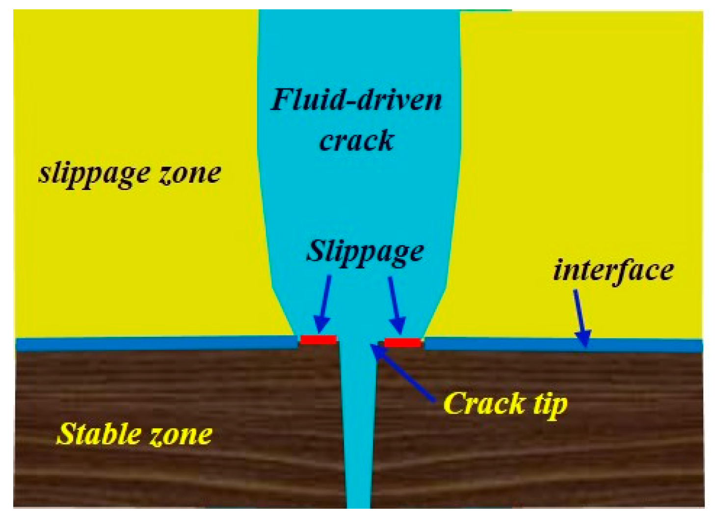
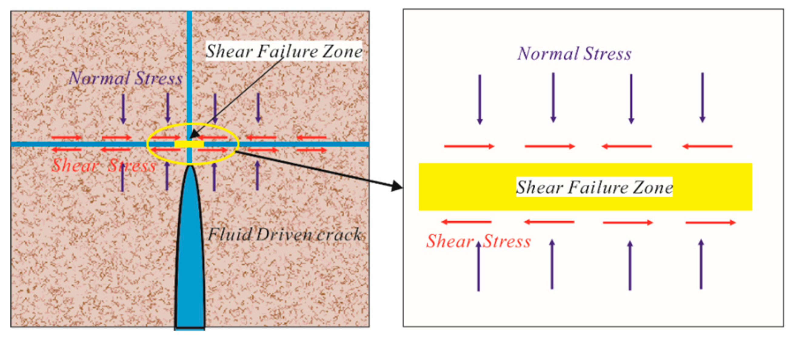
4.2.1. Shear Failure on Interface

According to Equation (2), shear strength is related to normal stress, and the stress state on the joint was calculated in Section 4.1. As mentioned above, normal stress decreased, and shear stress increased. The stress state of the joint (interface) is shown in Figure 12. Decreased normal stress can weaken the shear strength of the joint, whereas larger shear stress will increase the probability of shear failure. Therefore, when a fluid-driven fracture approaches the interface, slippage may occur due to shear failure of the interface, resulting in discontinuous displacement at the fracture tip.

With slippage caused by shear failure, the smaller the shear strength of the interface, the more it will be prone to slip. In fact, the reduction of normal stress and fluid action will lead to a reduction of shear strength. This will increase the probability of interface slippage.

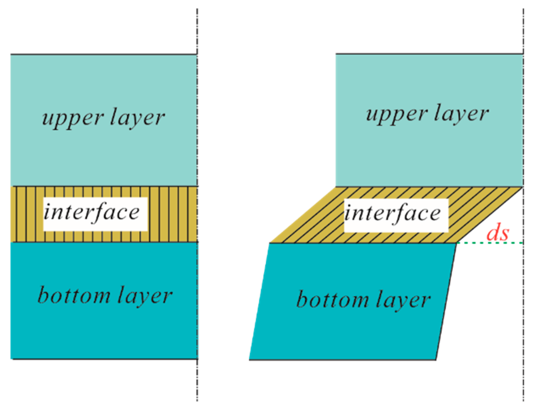
4.2.2. Discontinuous Deformation Caused by Interface

Shear failure of the interface is one of the reasons for fracture tip blunting. However, there are also slippage situations where the displacement is very small. In this situation, shear failure does not occur, but the fracture propagating perpendicular to the interface will still be hindered. There is another reason for discontinuous displacement: Discontinuous deformation between two zones on both sides of the interface is another explanation for interface slippage. Interface slippage is shown in Figure 13. To explain the effect of the interface, its thickness is shown to be larger than it actually is. There are upper and bottom layers above and below the interface. The mechanical strength of the upper and lower layers is much greater than that of the interface. With fluid pressure, there is only small displacement in the bottom layer, but the shear strain at the interface is large. As shown in Figure 13, there is a discontinuous displacement caused by the interface because the thickness is very small.

With slippage caused by discontinuous deformation, shear displacement of the interface is the key factor. According to Equation (1), shear displacement is related to shear stiffness coefficient Ks. A smaller Ks is more conducive to interface slippage.

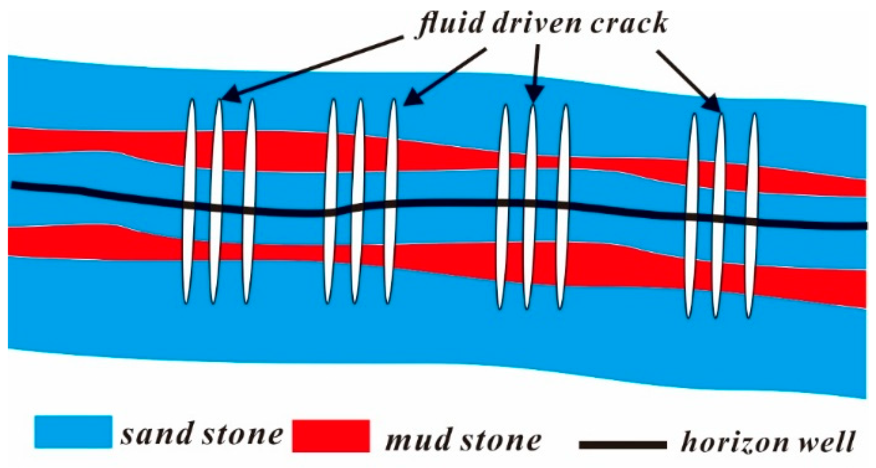
4.3. Manual Intervention of Interface Slippage in Hydraulic Fracture Containment

In conclusion, shear behavior is the fundamental reason for both shear failure and discontinuous displacement. Therefore, to analyze the effect of the interface on fracture containment, we should focus on the shearing behavior. During fracturing, manual intervention can be carried out mainly for two reasons: to change the stress state of the interface or to adjust the strength and stiffness of the interface.

For stress field reconstruction, if the fracture is expected to cross the interface, the normal stress needs to be increased, and the shear stress needs to be reduced. On the contrary, if the fracture is expected to be confined to the pay zone, normal stress should be reduced, and shear stress should be increased. By controlling the geometry of the adjacent fracture and the fluid pressure, we can artificially intervene in the stress [34]. In research on fracture direction control during secondary fracturing, there is a series of studies on the relationship between stress field reconstruction and fracture direction [35,36,37,38,39]. The results show that the stress can be changed by adjacent fractures to control the fracture direction. Of course, this problem still needs more discussion and study.

Interface slippage is related to shear strength and stiffness. Under the same stress conditions, the shear slippage of the interface will be larger when the shear stiffness is lower, and the interface is more prone to shear failure under low shear strength. Therefore, slippage will increase with lower shear strength and stiffness. As mentioned above, multilayer fracturing needs smaller slippage, whereas fracture containment needs larger slippage. Thus, higher shear strength and shear stiffness of the interface are required if the fracture is expected to cross the interface. Conversely, if the fracture needs to be confined to the pay zone, shear strength and shear stiffness need to be reduced. Fluid entering the formation will weaken its strength and stiffness. As the water saturation of the interface increases, the strength and stiffness decrease. An important aspect of manual intervention in interface properties is the viscosity of the fracturing fluid. Low-viscosity fluid is easier to filter into the interface, weakening its strength and stiffness [40,41]. However, fluid with too high a viscosity will increase the difficulty of injecting the fluid. Of course, in terms of interface alone, waterless fracturing technology is also an effective way to avoid weakening interface strength and stiffness. Therefore, to limit fractures to the pay zone, fracturing fluids with lower viscosity should be selected to reduce the strength and stiffness of the interface. On the contrary, to achieve multilayer fracturing, it is more appropriate to choose fracturing fluid with higher viscosity.

5. Conclusions

First, fracture height containment without stress contrast and distinct layer properties was studied with block discrete element. Then, the stress field on the interface was calculated by fracture mechanics with the same stress state and rock properties. Finally, the slippage forms, including shear failure and discontinuous displacement, at the interface were discussed. The main conclusions are as follows:

(1)

Interface slippage is one reason for fracture containment besides stress contrast and rock properties. Fracture containment still exists in the situation of the same stress state and rock properties, which means that fracture height containment still exists in one layer with a weak interface. Fracture tip blunting is the key factor that hinders fracture propagation. The mechanism of interface slippage is critical for fracture containment. The slippage forms on the interface include shear failure on the interface and discontinuous deformation caused by the interface.

(2)

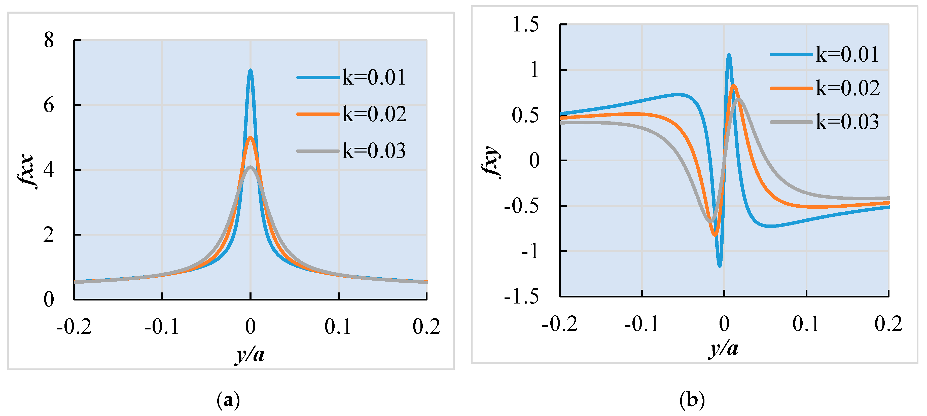
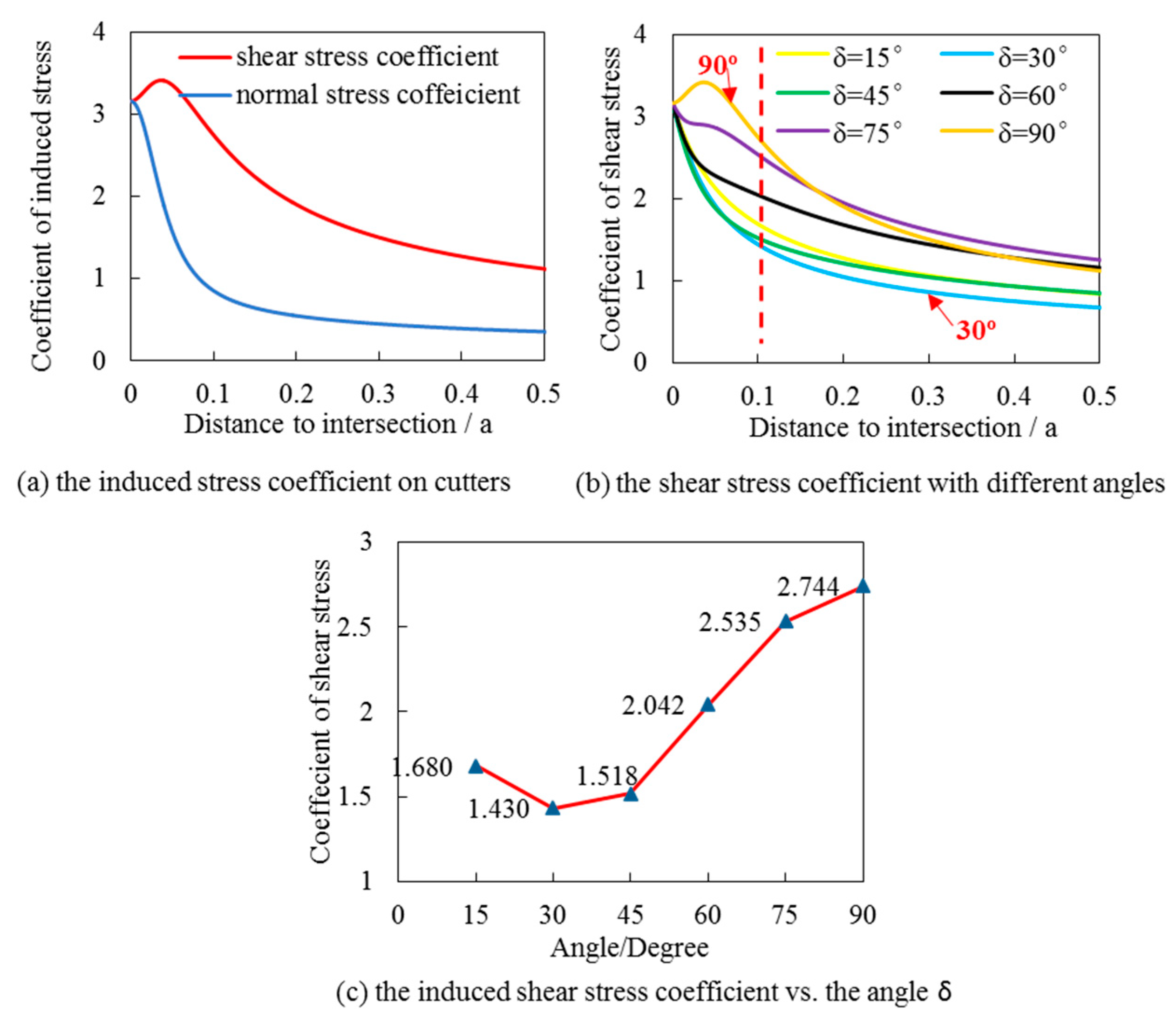
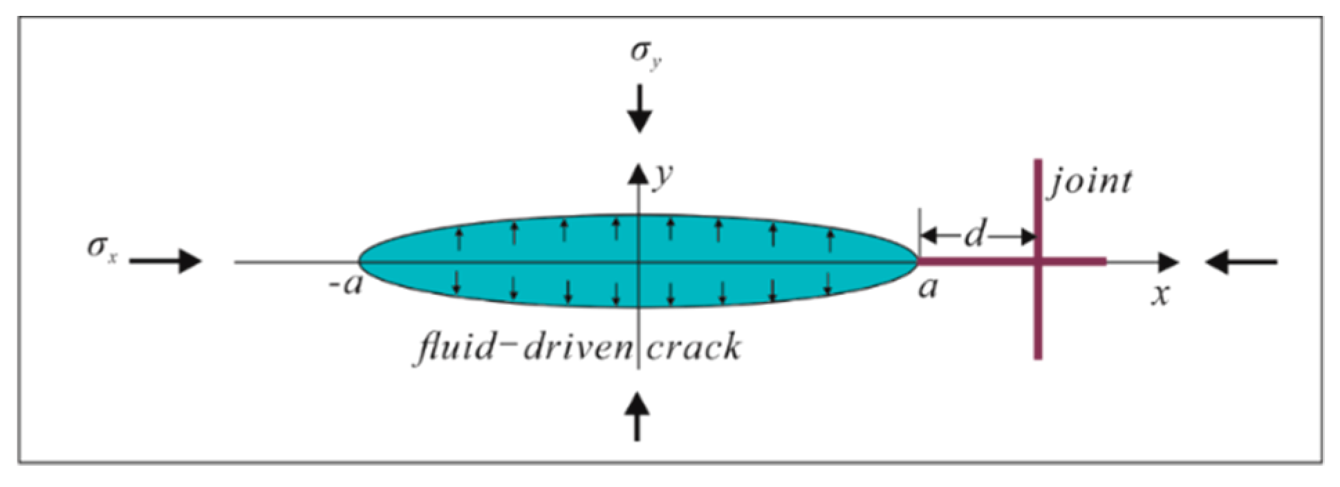
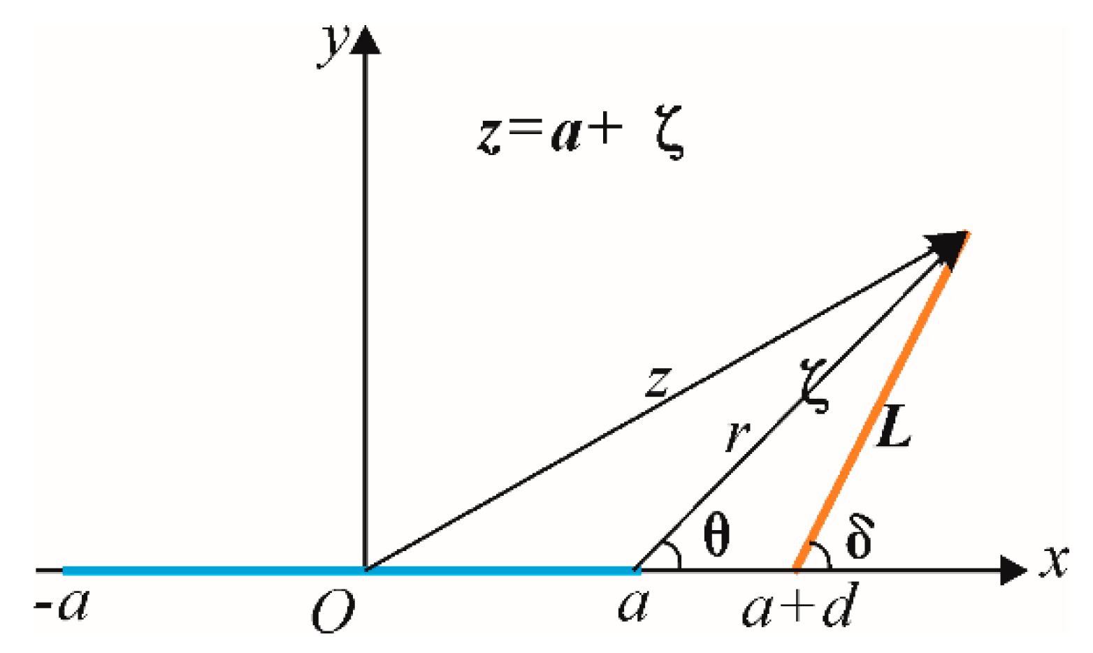
The coefficients of induced normal and shear stress were derived. The results show that induced stress can offset the original compressive stress and reduce the normal stress on joints, and shear stress in the range of 0.05 a is larger than the initial state. This indicates that hydraulic fracture will cause a reduction of normal stress and an increase of shear stress on joints.

(3)

According to the intended purpose, for hydraulic fracturing in pay zones or along multilayers, different measures, including manual intervention of stress, perforation angle, and fracturing fluid viscosity, are expected. For multilayer fracturing, fluid-driven fractures should be positioned at 30° to the interfaces by stress intervention and perforation angle, and shear stress should be increased, and normal stress reduced. Higher viscosity is appropriate. On the contrary, for pay zone fracturing, fluid-driven fractures should be adjusted to 90° to the interfaces by stress intervention and perforation angle, and shear stress should be decreased, and normal stress increased. Lower viscosity is appropriate.

References

1. Chuprakov, D.A.; Prioul, R. Hydraulic fracture height containment by weak horizontal interfaces. In Proceedings of the SPE Hydraulic Fracturing Technology Conference, Woodland, TX, USA, 3–5 February 2015; pp. 1–17. [Google Scholar]
2. Guo, J.; Luo, B.; Lu, C.; Lai, J.; Ren, J. Numerical investigation of hydraulic fracture propagation in a layered reservoir using the cohesive zone method. Eng. Fract. Mech. 2017, 186, 195–207. [Google Scholar] [CrossRef]
3. Xing, P.; Bunger, A.; Yoshioka, K.; Adachi, K.; El-Fayoumi, A. Experimental study of hydraulic fracture containment in layered reservoirs. In Proceedings of the 50th US Rock Mechanics/Geomechanics Symposium, Houston, TX, USA, 26–29 June 2016. [Google Scholar]
4. Weng, X.; Chuprakov, D.; Kresse, O.; Prioul, R.; Wang, H. Hydraulic fracture-height containment by permeable weak bedding interfaces. Geophysics 2018, 83, MR137–MR152. [Google Scholar] [CrossRef]
5. Xiangjun, C.; Langfeng, M.; Zhongbao, W.; Yiqun, Y.; Yang, Z.; Linlin, S. Calculating method of the productivity for the trans-layer fractured horizontal well. Pet. Geol. Oilfield Dev. Daqing 2019, 3, 65–72. [Google Scholar] [CrossRef]
6. Simonson, E.; Abou-Sayed, A.; Clifton, R. Containment of massive hydraulic fractures. Soc. Pet. Eng. J. 1978, 18, 27–32. [Google Scholar] [CrossRef]
7. Van Eekelen, H. Hydraulic fracture geometry: fracture containment in layered formations. Soc. Pet. Eng. J. 1982, 22, 341–349. [Google Scholar] [CrossRef]
8. Fung, R.; Vilayakumar, S.; Cormack, D.E. Calculation of vertical fracture containment in layered formations. SPE Form. Eval. 1987, 2, 518–522. [Google Scholar] [CrossRef]
9. Daneshy, A. Hydraulic fracture propagation in layered formations. Soc. Pet. Eng. J. 1978, 18, 33–41. [Google Scholar] [CrossRef]
10. Warpinski, N.R.; Schmidt, R.A.; Northrop, D.A. In-situ stresses: The predominant influence on hydraulic fracture containment. J. Pet. Technol. 1982, 34, 653–664. [Google Scholar] [CrossRef]
11. Warpinski, N.R.; Clark, J.A.; Schmidt, R.A.; Huddle, C.W. Laboratory investigation on the effect of in situ stresses on hydraulic fracture containment. Soc. Pet. Eng. J. 1982, 22. [Google Scholar] [CrossRef]
12. Teufel, L.W.; Clark, J.A. Hydraulic-fracture propagation in layered rock: Experimental studies of fracture containment. Soc. Pet. Eng. J. 1981. [Google Scholar] [CrossRef]
13. Zhang, F.; Dontsov, E. Modeling hydraulic fracture propagation and proppant transport in a two-layer formation with stress drop. Eng. Fract. Mech. 2018, 199, 705–720. [Google Scholar] [CrossRef]
14. Wasantha, P.; Konietzky, H.; Xu, C. Effect of in-situ stress contrast on fracture containment during single-and multi-stage hydraulic fracturing. Eng. Fract. Mech. 2019, 205, 175–189. [Google Scholar] [CrossRef]
15. Huang, J.; Ma, X.; Shahri, M.; Safari, R.; Yue, K.; Mutlu, U. Hydraulic fracture growth and containment design in unconventional reservoirs. In Proceedings of the 50th US Rock Mechanics/Geomechanics Symposium, Houston, TX, USA, 26–29 June 2016. [Google Scholar]
16. Xu, W.; Prioul, R.; Berard, T.; Weng, X.; Kresse, O. Barriers to hydraulic fracture height growth: A new model for sliding interfaces. In Proceedings of the SPE Hydraulic Fracturing Technology Conference and Exhibition, Woodlands, TX, USA, 5–7 February 2019. [Google Scholar]
17. Xing, P.; Yoshioka, K.; Adachi, J.; El-Fayoumi, A.; Bunger, A.P. Laboratory demonstration of hydraulic fracture height growth across weak discontinuitiesHF height growth with weak interfaces. Geophysics 2018, 83, MR93–MR105. [Google Scholar] [CrossRef]
18. Wang, H.; Liu, H.; Wu, H.A.; Wang, X.X. A 3D numerical model for studying the effect of interface shear failure on hydraulic fracture height containment. J. Pet. Sci. Eng. 2015, 133, 280–284. [Google Scholar] [CrossRef]
19. Tang, J.; Wu, K. A 3-D model for simulation of weak interface slippage for fracture height containment in shale reservoirs. Int. J. Solids Struct. 2018, 144, 248–264. [Google Scholar] [CrossRef]
20. Gil, I.; Nagel, N.; Sanchez-Nagel, M.; Damjanac, B. The effect of operational parameters on hydraulic fracture propagation in naturally fractured reservoirs-getting control of the fracture optimization process. In Proceedings of the 45th US Rock Mechanics/Geomechanics Symposium, San Francisco, CA, USA, 26–29 June 2011. [Google Scholar]
21. Cundall, P.A. Formulation of a three-dimensional distinct element model—Part I. A scheme to detect and represent contacts in a system composed of many polyhedral blocks. Int. J. Rock Mech. Min. Sci. Geomech. Abstr. 1988, 25, 107–116. [Google Scholar] [CrossRef]
22. Hart, R.; Cundall, P.; Lemos, J. Formulation of a three-dimensional distinct element model—Part II. Mechanical calculations for motion and interaction of a system composed of many polyhedral blocks. Int. J. Rock Mech. Min. Sci. Geomech. Abstr. 1988, 25, 117–125. [Google Scholar] [CrossRef]
23. Zhang, Z.; Chen, F.; Li, N.; He, M. Influence of fault on the surrounding rock stability for a mining tunnel: Distance and tectonic stress. Adv. Civ. Eng. 2019, 2019. [Google Scholar] [CrossRef]
24. Zhu, J.B.; Liao, Z.Y.; Tang, C.A. Numerical SHPB tests of rocks under combined static and dynamic loading conditions with application to dynamic behavior of rocks under in situ stresses. Rock Mech. Rock Eng. 2016, 49, 3935–3946. [Google Scholar] [CrossRef]
25. Zheng, Y.; Liu, J.; Lei, Y. The propagation behavior of hydraulic fracture in rock mass with cemented joints. Geofluids 2019, 2019. [Google Scholar] [CrossRef]
26. Goodman, R.E.; Taylor, R.L.; Brekke, T.L. A model for the mechanics of jointed rock. J. Soil Mech. Found. Div. 1968, 94, 637–660. [Google Scholar]
27. Deng, C.; Kong, W.; Zheng, Y. Analysis of the ultimate bearing capacity of jointed rock foundations by fem. Ind. Constr. 2005, 35, 51–54. [Google Scholar]
28. Youjun, J.; Jie, W.; Liuke, H. Analysis on inflowing of the injecting water in faulted formation. Adv. Mech. Eng. 2015, 7. [Google Scholar] [CrossRef]
29. Itasca Consulting Group Inc. Available online: https://www.itascacg.com/software/3dec (accessed on 1 June 2019).
30. Zhao, Z.; Kim, H.; Haimson, B. Hydraulic fracturing initiation in granite. In Proceedings of the 2nd North American Rock Mechanics Symposium, Montreal, QC, Canada, 19–21 June 1996. [Google Scholar]
31. Bai, M.; Green, S.; Casas, L.; Miskimins, J. 3-D simulation of large-scale hydraulic fracturing tests. In Proceedings of the 41st US Rock Mechanics Symposium, Golden, CO, USA, 17–21 June 2006. [Google Scholar]
32. Kim, G.H.; Wang, J.Y. Interpretation of hydraulic fracturing pressure in low-permeability gas formations. In Proceedings of the SPE Production and Operations Symposium, Oklahoma City, OK, USA, 27–29 March 2011. [Google Scholar]
33. Shiyu, L. , Taiming, H., Xiangchu, Y. Fracture Mechanics of Rock; Science Press: Beijing, China, 2016. [Google Scholar]
34. Zheng, Y.; Liu, J.; Zhang, B. Artificial interference of stress field in a near-fracture zone by water injection in a preexisting crack. Adv. Civil Eng. 2019, 2019. [Google Scholar] [CrossRef]
35. Zhang, G.Q.; Chen, M. Dynamic fracture propagation in hydraulic re-fracturing. J. Pet. Sci. Eng. 2010, 70, 266–272. [Google Scholar] [CrossRef]
36. Gao, Q.; Cheng, Y.; Han, S.; Yan, C.; Jiang, L. Numerical modeling of hydraulic fracture propagation behaviors influenced by pre-existing injection and production wells. J. Pet. Sci. Eng. 2019, 172, 976–987. [Google Scholar] [CrossRef]
37. Chen, S.; Sun, Q.; Song, Z. Changes of ground stress field and development policy in later half period of water injection for the extremely low permeability reservoirs with fractures. Geoscience 2008, 4, 647–654. [Google Scholar]
38. Wright, C.; Conant, R.; Golich, G.M.; Bondor, P.L.; Murer, A.S.; Dobie, C.A. Hydraulic fracture orientation and production/injection induced reservoir stress changes in diatomite waterfloods. Poceedings of the SPE Western Regional Meeting, Bakersfield, CA, USA, 8–10 March 1995. [Google Scholar]
39. Manríquez, A.L. Stress behavior in the near fracture region between adjacent horizontal wells during multistage fracturing using a coupled stress-displacement to hydraulic diffusivity model. J. Pet. Sci. Eng. 2018, 162, 822–834. [Google Scholar] [CrossRef]
40. Tan, P.; Jin, Y.; Han, K.; Hou, B.; Chen, M.; Gou, J. Analysis of hydraulic fracture initiation and vertical propagation behavior in laminated shale formation. Fuel 2017, 206, 482–493. [Google Scholar] [CrossRef]
41. Beugelsdijk, L.J.L.; de Pater, C.J.; Sato, K. Experimental hydraulic fracture propagation in a multi-fractured medium. In Proceedings of the SPE Asia Pacific Conference on Integrated Modelling for Asset Management, Yokohama, Japan, 25–26 April 2000. [Google Scholar]
Figure 1. Fracture containment in pay zone.
Energies 12 03245 g001
Figure 2. Translayer fracturing in interbed of sandstone and mudstone.
Energies 12 03245 g002
Figure 3. Three-dimensional model of rock with two horizontal joints and one vertical joint: (a) the model of joint; (b) the model with blocks and joints.
Energies 12 03245 g003
Figure 4. Geometric profiles of fluid-driven fractures at different times: (a) 21 s, (b) 80 s, (c) 110 s, and (d) 140 s; and normal displacement on (e) the upper horizontal joint and (f) the bottom horizontal joint.; (g) the curves of injection pressure.
Energies 12 03245 g004
Figure 5. Results of numerical simulation: (a) shear stress on horizontal joint; (b) normal stress on horizontal joint; (c) aperture curves along vertical line passing through center point of vertical joint; (d) geometries of fractures at different steps.
Energies 12 03245 g005
Figure 6. Interface slippage at fracture tip.
Energies 12 03245 g006
Figure 7. Model diagram of fractures with fluid pressure.
Energies 12 03245 g007
Figure 8. Polar coordinate system of fracture front of orthogonal joint.
Energies 12 03245 g008
Figure 9. Induced stress coefficient of joint at fracture front of (a) normal stress; (b) shear stress.
Energies 12 03245 g009
Figure 10. Polar coordinate system of fracture front of nonorthogonal joint.
Energies 12 03245 g010
Figure 11. Induced stress coefficient on cutters of (a) shear and normal stress (δ = 90º), (b) shear stress with different angles, and (c) with angle δ.
Energies 12 03245 g011
Figure 12. Shear model of interface.
Energies 12 03245 g012
Figure 13. Discordant deformation (ds) caused by interface.
Energies 12 03245 g013