Improvement of Short-Term BIPV Power Predictions Using Feature Engineering and a Recurrent Neural Network

Abstract

The time resolution and prediction accuracy of the power generated by building-integrated photovoltaics are important for managing electricity demand and formulating a strategy to trade power with the grid. This study presents a novel approach to improve short-term hourly photovoltaic power output predictions using feature engineering and machine learning. Feature selection measured the importance score of input features by using a model-based variable importance. It verified that the normative sky index in the weather forecasted data had the least importance as a predictor for hourly prediction of photovoltaic power output. Six different machine-learning algorithms were assessed to select an appropriate model for the hourly power output prediction with onsite weather forecast data. The recurrent neural network outperformed five other models, including artificial neural networks, support vector machines, classification and regression trees, chi-square automatic interaction detection, and random forests, in terms of its ability to predict photovoltaic power output at an hourly and daily resolution for 64 tested days. Feature engineering was then used to apply dropout observation to the normative sky index from the training and prediction process, which improved the hourly prediction performance. In particular, the prediction accuracy for overcast days improved by 20% compared to the original weather dataset used without dropout observation. The results show that feature engineering effectively improves the short-term predictions of photovoltaic power output in buildings with a simple weather forecasting service.

1. Introduction

The development of technologies to harvest renewable forms of energy, such as solar photovoltaics and wind power generators, is in fact one of the key drivers for their implementation in microgrids, interconnected with the grid, to trade generated electricity [1]. Although clean technologies address the need for sustainable energy, their inherent variability and dependence on weather conditions complicate the management of the power network [2]. Consequently, it is only prudent to require that earlier methods, which have always been used to balance power generation and consumption, be updated to incorporate these complications [3]. For example, to address the variability in the power demand on microgrids, the first step must be to predict the short-term load demand [4,5]. This is necessary to obtain the amount of energy that will be consumed to efficiently balance the supply and demand sides of a system with power generators. The second step is to predict the energy generated by renewable energy sources, in order to continuously update the status of the power network. For example, solar power generation is known to be directly related to onsite weather conditions [2]. Therefore, solar power is not only diurnal in nature but also varies throughout the day with changes in the solar irradiation [6]. Photovoltaic (PV) power output predictions require precursor knowledge of the weather parameters.

Different models and parameters that are known to have an influence, such as cloudiness and solar irradiance, have been used for PV power output prediction [7]. Previous research has suggested that the prediction of renewable energy generation is an approach to balance supply and demand in electricity energy management [1,8,9].

In recent years, numerous prediction methods for PV power systems have been developed with the use of statistical models and machine-learning algorithms. Researchers have attempted to overcome many difficulties to present accurate methods to predict PV power output. Several prediction methods have had different levels of success in improving the accuracy and reducing the complexity in terms of computational cost. These methods can be categorized into direct and indirect.

Indirect prediction methods estimate the PV power output by using or predicting the solar irradiance over different time scales. They can use numerical weather forecast information, image processing, and statistical and hybrid artificial neural networks to predict solar irradiance [10]. Several hybrid models have been proposed to predict PV power output based on the indirect method. Filipe et al. [11] suggested a combination of hybrid solar power prediction methods, consisting of both statistical and physical methods. In other words, an electrical model of a PV system is combined with a statistical model that converts numerical weather forecasted data into solar power with a short-term predictive horizon for the physical model. Dong et al. [12] developed a hybrid prediction method for hourly solar irradiance by integrating self-organizing map, support vector regression, and particle swarm optimization approaches. Alternatively, PV power can be predicted using the indirect method with the aid of simulation tools, such as TRNSYS, PVFORM, and HOMER [13]. Although many indirect approaches have been developed, the prediction accuracy depends on the accuracy of solar irradiation predictions. However, the prediction performance of solar irradiation is still not good because of the quality of forecasted weather data [14]. It also has limited applicability for typical buildings that do not have solar meters to measure the various forms of solar irradiation, such as direct normal irradiance (DNI) or global horizontal irradiance (GHI).

Direct prediction methods employ historical PV power generation data and forecasted weather conditions that generally do not include solar irradiation. Several studies have reviewed the methods that enhance building-integrated photovoltaic (BIPV) power prediction using ensemble methods. Wan et al. [15] analyzed different PV power and solar irradiance prediction techniques. Raza et al. [16] focused on PV power prediction models. Gandoman et al. [17] evaluated the prediction performance of PV power output based on the short-term influences of cloud cover. Machine learning was used to develop direct prediction methods. Shi et al. [18] developed a 1-day-ahead PV power output prediction based on a support vector machine (SVM) and the features of weather categorization at a PV station in China. Mellit et al. [19] proposed a short-term prediction of meteorological time-series parameters using the least squares SVM. Although numerous studies have suggested the prediction of PV power output using various prediction algorithms and hybrid models based on the direct method, conventional direct methods have limited ability to maintain a high hourly prediction performance of short-term PV power output because these models mainly depend on forecasted weather data, which does not include solar irradiance. In addition, prior studies have focused on the type of algorithm and configuration of the particular models to improve the prediction accuracy. Therefore, both input features, such as weather information, and the prediction model configuration must be considered to improve the hourly prediction accuracy.

This study proposes an improved method for short-term prediction of BIPV power generation with simple weather forecast data using feature engineering and machine learning. First, feature selection is performed by using the weather forecast parameters to identify the impact of input variables used for BIPV prediction by taking into account the importance of each variable. The BIPV prediction performance of several machine-learning algorithms are then compared to select an appropriate model.

This study is organized as follows: Section 2 introduces the framework of the prediction models and performance improvement techniques. Section 3 characterizes the weather features by variable importance. Section 4 discusses the prediction performance with several machine-learning models. The main results of the improvement techniques are presented in Section 5 and the conclusions appear in Section 6.

2. Methodology

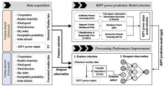
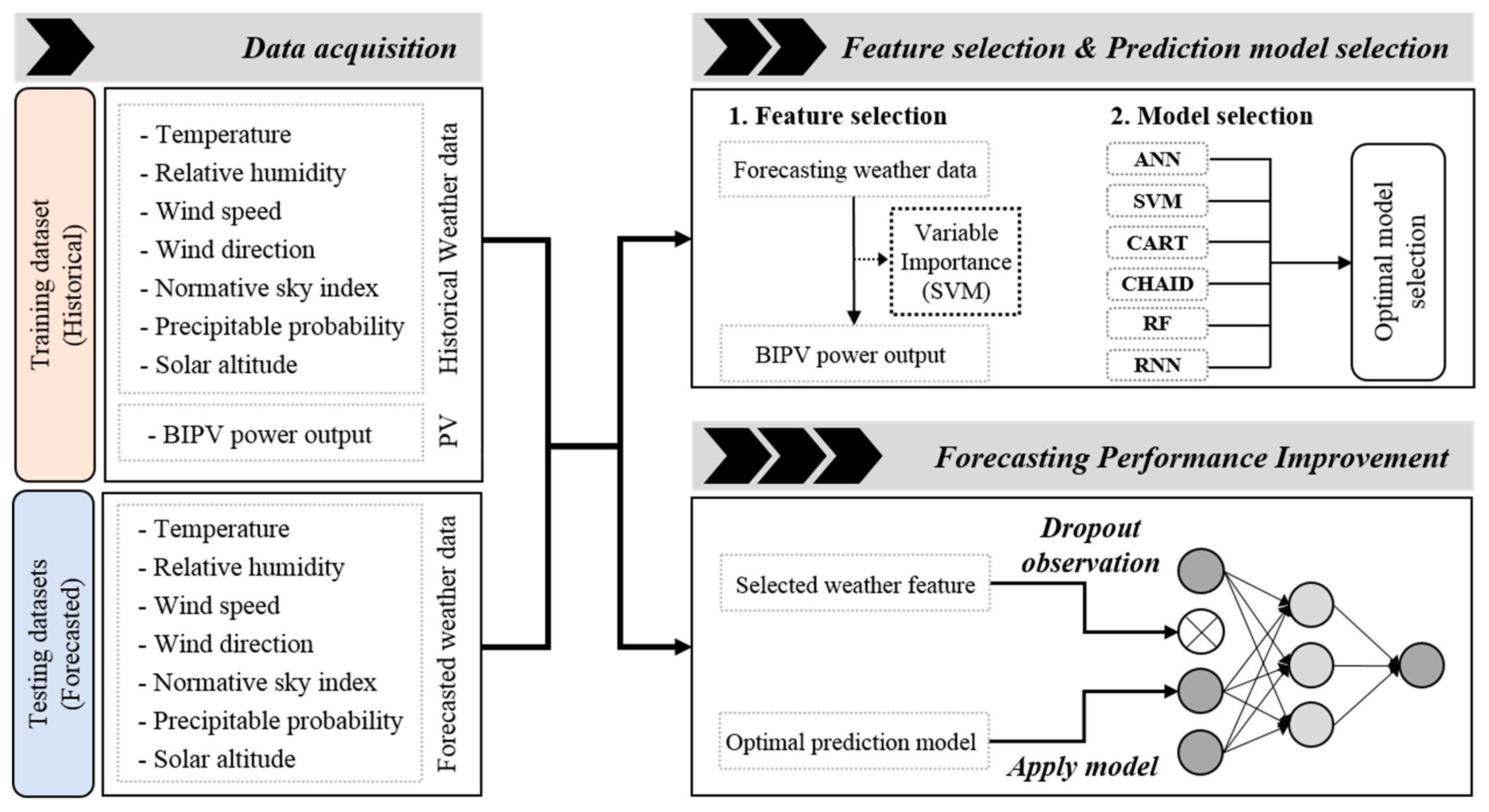
The proposed short-term prediction model for BIPV power systems is a combination of a feature engineering technique and machine-learning model. Figure 1 shows the framework, which is composed of three steps: data acquisition, the selection of a machine-learning model for BIPV power output prediction, and a technique to improve the prediction performance. First, training (historical) and testing (forecasted) datasets were constructed by collecting data from the online weather service and historical hourly PV power outputs. Second, the lowest correlated feature in the weather forecast data was selected by feature selection, then the most optimal BIPV prediction model was selected by comparing six conventional machine-learning models using the original input data set. Finally, this study suggests a method to improve prediction accuracy by using the dropout observation algorithm, one of the feature engineering approaches.

2.1. Characteristics of the BIPV

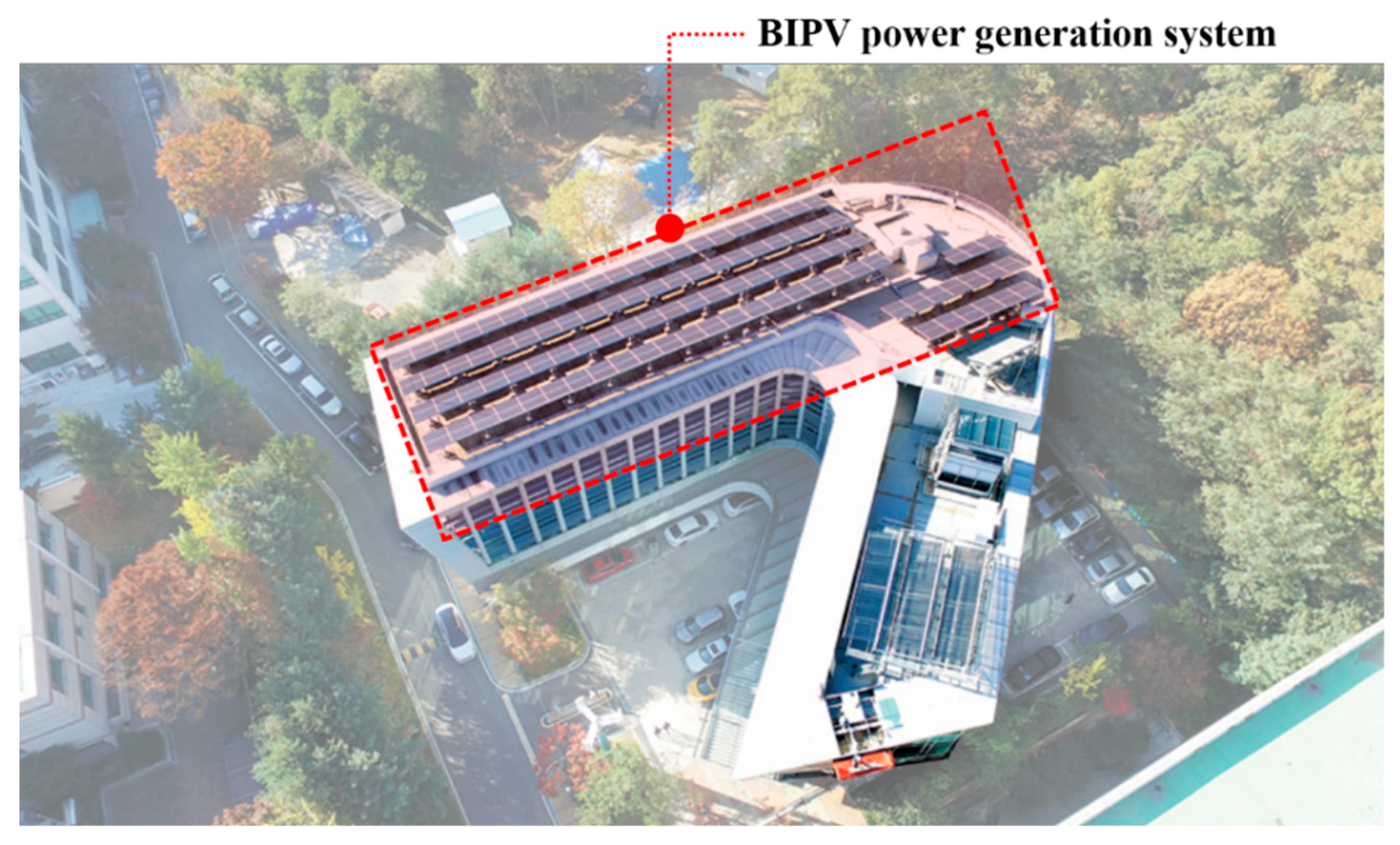
Photovoltaic power generation systems were installed on the roof of a medium-sized office building in South Korea at a latitude 37°31′N and longitude 127°14′E, as shown in Figure 2. The capacity of this photovoltaic generation system is approximately 50 kW and the specifications of the BIPV system are listed in

Table 1. Specifications of the BIPV generation system.

Element	Parameters
Module type	SM-250PG8 (Grid-connected)
Connection type	10 series × 20 parallel
Nominal module efficiency	15.03%

. The BIPV power was measured in minutes and then aggregated into a relational database management system (RDBMS). For the purpose of short-term prediction, this study collected hourly BIPV power measurements from June 2017 to August 2018.

2.2. Description of Predictors

The forecasted weather dataset containing the historical weather data was obtained from the Korea Meteorological Administration (KMA) and Korea Astronomy and Space Science Institute (KASI). Seven weather variables were used as predictors: outdoor air temperature (OT), relative humidity (RH), wind direction (WD), wind speed (WS), normative sky index (NSI), precipitation (PP), and solar altitude (SA). The entire set of weather variables consists of data collected at 3-hour intervals. In this study, these variables, with 3-hour resolution, were pre-processed by converting them to an hourly resolution to perform the short-term prediction for the hourly BIPV power system.

2.3. Prediction Algorithms

BIPV power output mainly depends on the input variables (i.e., weather data and system characteristics) and prediction model. The performance of the prediction model is affected by the model configuration and type. This study assessed six machine-learning models, i.e., an artificial neural network (ANN), support vector machine (SVM), classification and regression tree (CART), chi-square automatic interaction detection (CHAID), random forest (RF), and recurrent neural network (RNN), with the objective of selecting an appropriate prediction model. Each prediction model is implemented with MATLAB (version R2016b, MathWorks, USA) with Windows 10.

The ANN model, which is effective when solving nonlinear problems, has a structure that consists of an input layer, hidden layers, and one output layer. Learning occurs by assigning weights and bias to each layer [20]. Various neural network models exist, which differ in terms of their learning process, model structure, and other features. Among these models, a feed-forward neural network (FFNN) with back-propagation was selected for this study because of its simple model configuration and computational speed. FFNN functions by relocating the information in the former layer to the next layer in a forward direction [21]. In addition, FFNN has a hyperbolic tangent function, which is used to transfer the trained information from the hidden layer to the output layer.

The SVM has been widely applied for pattern recognition (e.g., classification and regression problems). SVM uses a hyperplane and margin to identify the support vectors of the datasets. In particular, the original datasets are mapped into higher dimensional space to classify them using kernel functions capable of effectively solving nonlinear classification problems [22]. Here, a radial basis function (RBF) is applied, which has been proven to outperform kernel functions due to its computational efficiency, simplicity, and reliability compared with other functions [23].

Among the various algorithms based on the decision trees, the CART and CHAID models are the most popular algorithms. These nonparametric methods can be used to process various data types, such as nominal, ordinal, and continuous variables [24]. The two models differ significantly. The CART model grows the next tree by splitting two child nodes. The main predictor is generated by measuring an impurity or diversity. CHAID constructs multiple split nodes and performs statistical tests when each node is split [25].

The RF is an ensemble-learning algorithm that solves both classification and regression problems. Previous studies, especially in recent years, have shown that this algorithm is capable of solving real-world problems in many fields. In particular, RF is a more robust model than models based on a single decision tree, such as CART and CHAID, because several decision tree models are used and then combined using a bootstrap. Furthermore, each tree with the lowest error rate is replaced in the original dataset before the next tree is grown [26,27].

The RNN [28] is a modification of the ANN and has a circulated connection between nodes of layers to maintain an inner state, compared with feed forward connections. The circulated connection allows the network to act on information from previous steps in the computational sequence; thus, it exhibits dynamic temporal behavior. This characteristic makes RNNs advantageous to use for the analysis of sequential data. Applying dropout to a neural network amounts to sampling a “thinned” network from it. As a recurrent neural network, long short-term memory (LSTM) cells were used, which solve the problem of a vanishing gradient during training in this study. LSTM cells contain an explicit state. The value stored in this state is then regulated by gates within the cell. These gates have specific rules that define when to store, update, or forget the value in the internal state [29]. Considering model constitution, RNN is an appropriate model for time series prediction.

To determine the optimal conditions for each machine-learning model, cross-validation was implemented with different parameters based on [30] in MATLAB. The obtained configurations of each prediction model are listed in

Table 2. The specified conditions for each of the six machine-learning models.

Model	Configuration Parameters	Range/Type	Selected Parameter
Artificial neural network (ANN)	Activation function	Sigmoid, Hyperbolic tangent, Rectified linear unit	Hyperbolic tangent
	Number of hidden neurons	7 ~ 15	10
	Data division (training/testing)	80%/20%, 70%/30%	70%/30%
Support vector machine (SVM)	Kernel type	Polynomial, RBF, Sigmoid	RBF
	RBF Gamma	−0.5 ~ +0.5	+0.1
	Gamma	−3.0 ~ +3.0	+1.0
	Regression precision(epsilon)	−0.5 ~ +0.5	0.1
Classification and decision tree (CART)	Tree depth	1 ~ 11	5
	Minimum change in impurity	1 ~ 0.0001	0.0001
	Impurity measure	Entropy, Gini	Gini
	Overfit prevention set	20% ~ 30%	30%
Chi-square automatic interaction detection (CHAID)	Tree depth	1 ~ 11	4
	Minimum change in expected cell frequencies	1 ~ 0.001	0.001
	Maximum iterations for convergence	50 ~ 150	100
Random forest (RF)	Number of nodes	10 ~ 10,000	10,000
	Tree depth	1 ~ 11	10
	Child node size	5	5
Recurrent neural network(RNN)	Activation function	Sigmoid, Hyperbolic tangent, Rectified linear unit	Hyperbolic tangent
	Number of hidden neurons	7 ~ 15	10
	Data division (training/testing)	80%/20%, 70%/30%	70%/30%

.

2.4. Variable Importance

Variable importance analysis is required to determine which variables contain noise that would prevent accurate prediction. Variable importance analysis is a key pre-processing step for any appropriate prediction method. It is important to identify the potential predictors that have a high impact on the function response. The use of SVM for variable importance analysis was applied for this study.

Among the model-based variable importance approaches such as linear models, random forests, and bagged/boosted trees, SVM has been reported as a high performance in many classification and prediction problems due to its strong generalization ability and robust feature selection method [31,32,33]. Variable importance analysis with SVM uses gradient descent to minimize generalization bounds. The SVM develops an optimal hyperplane in the dimensional space of $x \in R^n$ into a high (possibly infinite) dimensional space and constructs an optimal hyperplane in this space [34]. The decision function of the SVM classification for a new sample of x is defined by Equation (1).

$$f\left(x\right)=W·\varnothing \left(x\right)+b={\displaystyle \sum }_i{\alpha }_i{y}_{i}K(x_i,x)+b$$

(1)

where $\varnothing \left(x\right)$ is the maximal margin function from the hyperplane, W is the weight, and b is the bias of the SVM decision function. K(x) is the kernel function, and ${\alpha }_i$ denotes Lagrange multipliers corresponding to primal constraints. $x_i$ denotes training vectors, and $y_i$ denotes the corresponding labels of $\pm 1$. The SVM attempts to find the function from the dataset, by solving Equation (2) with Lagrange multipliers, it can reduce to maximizing the following optimization problem.

$$W^2\left(\alpha \right)={\displaystyle \sum }_{i=1}^l{\alpha }_i-\frac{1}{2}{\displaystyle \sum }_{i,j=1}^l{\alpha }_i{\alpha }_j{y}_i{y}_{j}K\left(x_i,x_j\right)$$

(2)

The SVM is used for analyzing the input variables and output variables by changing the cost function. The SVM identifies the variable importance by using the gradient of weight (∆W) between the weight with the specific variable and that without the variable given by Equation (3). A larger change in the weight illustrates that the specific variable impacts the result more.

$$∆W=\left|W-W_{\mathrm{witout}\mathrm{specific}\mathrm{variable}}\right|$$

(3)

2.5. Observation Dropout

The most popular method for network regularization is dropout, which randomly selects certain activation portions in networks. Dropout regularizes data by removing layers or nodes in the neural network [35].

Different dropout models were initially developed to improve the manner in which strong networks can facilitate the interpretation of decisions, e.g., the assignment of a particular label to an image similar to the one in question [36,37,38]. A number of studies have highlighted the use of various dropout methods as a way to improve model performance [39]. Kingma et al. [40] proposed the Bayes form of interpretation [41] by compressing the architectural model [42]. These proposals were aimed at transforming the rate of dropout to optimize model performance. The units that remain after the dropout are those that form the network. Dropout is commonly used for regularization to enhance the performance. The dropout observation method was introduced to analyze which features are relevant for a predicted target variable.

Observation dropout is used in the algorithm proposed in this study based on feature dropout [43] of the neural network models. When using feature dropout, specific feature vectors are allocated noise with the dropout procedure for each training instance, where the noise is randomly allocated to data that has a specific probability or zero as its value. The effects of feature dropout may maximize the performance contribution of other features based on the proposed neural network model [44].

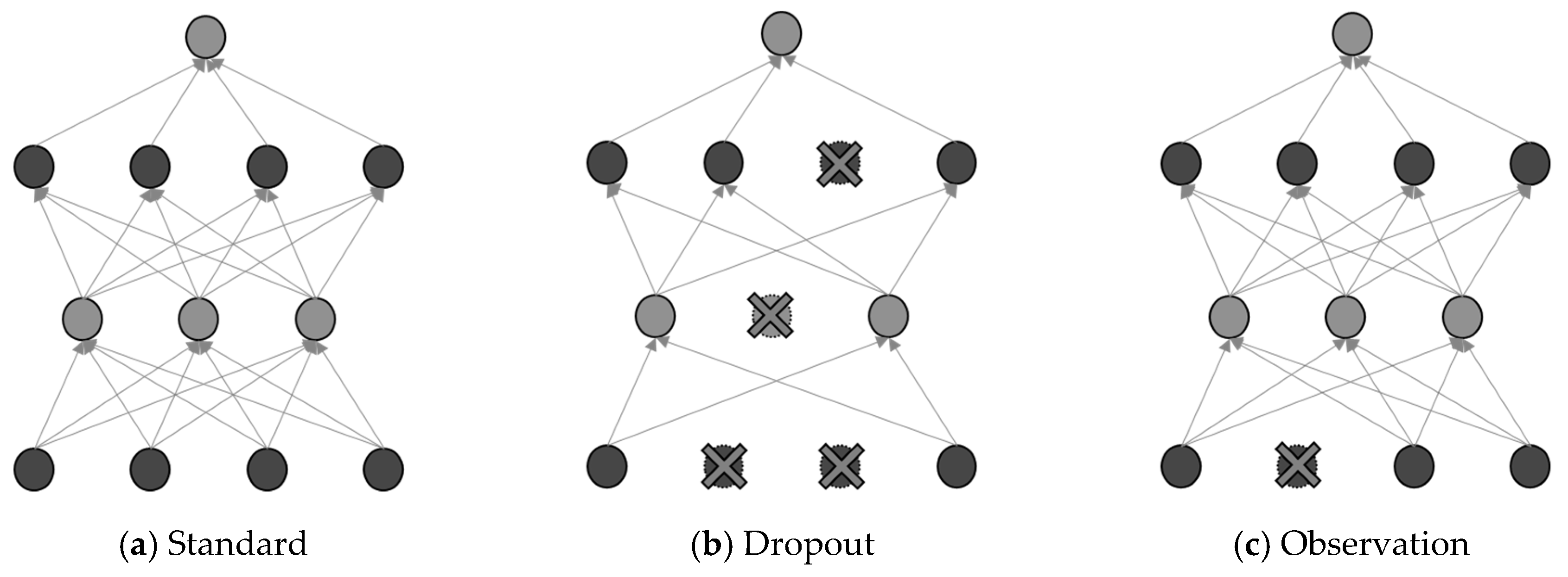
However, in this study, compared with the original feature dropout technique, several observations with specific probabilities in the specific feature for each training instance were removed, as shown in Figure 3. The removal of certain data in the specific feature implies that the addition of noise to unrelated data improves the performance, which has an identical effect as using the dropout in the neural network methods. SVM identified the lowest correlated feature by considering the importance of each variable. Then, a regularization method was applied to the specific feature such that its value became zero in the training and prediction process with a probability of p.

These units, n, can be used for a hyper parameter to define the number of neural nets. In the presentation of each training case, a thinned network is trained and sampled. This indicates that, when a neural network is trained with dropout, it is equivalent to training 2ⁿ networks that are thinned and share the weight. In doing so, thinned networks are largely prevented from becoming strained. After a certain time, clearly estimating the different models that were thinned would become unsustainable. Nevertheless, a simple approach to estimation can be effective. It is logical to use one neural network at a time in the absence of dropout. The pressure exerted by these network forms is a representation of strained weights. In the event that a given unit is strained with a possibility, p, at the time of training, the outgoing weights for that unit are increased by p at the time of the prediction. This ensures that any output that was hidden is similar to the exact output at the time of the prediction. When scaling is implemented, 2ⁿ nets, whose weights are shared, are collected to form one neural network for the prediction time. Training networks with dropout, as well as the use of proper averaging procedures at the prediction time, have been found to reduce the number of errors due to generalization, for numerous classification challenges when compared with the use of other methods of training regularization [35].

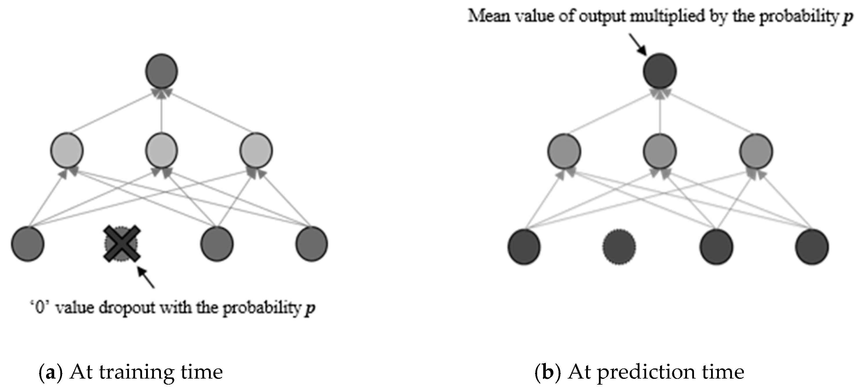
In this methodology, during training, random probabilities are multiplied with a specific feature of the input training data to achieve dropout, which yields an approximate averaging method of the regularization at the prediction time using probability, p, and that without the regularization (1 − p) as shown in Figure 4.

3. Feature Selection by Variable Importance

As described in Section 2.4, the SVM measures the importance scores by the prediction performance, incorporating the correlation structure between the forecasted weather variables.

Table 3. The variable importance score of weather variables based on SVM.

	Daily Sky Conditions
	Clear Days (15 Days)	Slightly Cloudy Days (14 Days)	Cloudy Days (17 Days)	Overcast Days (18 Days)
OT	0.07	0.04	0.03	0.03
RH	0.20	0.22	0.16	0.18
WS	0.01	0.04	0.01	0.02
WD	0.02	0.01	0.00	0.01
NSI	0.01	0.01	0.00	0.00
PP	0.00	0.00	0.04	0.01
SA	0.69	0.65	0.79	0.75

Summation of the importance score with measured values is 1.

provides the importance score of each weather feature based on the historical dataset for the four types of daily sky conditions. SA had the highest importance score for all sky conditions among the variables. Cloudier skies correspond to higher variable importance scores for SA due to the correlation between BIPV power generation and the angle of solar irradiation.

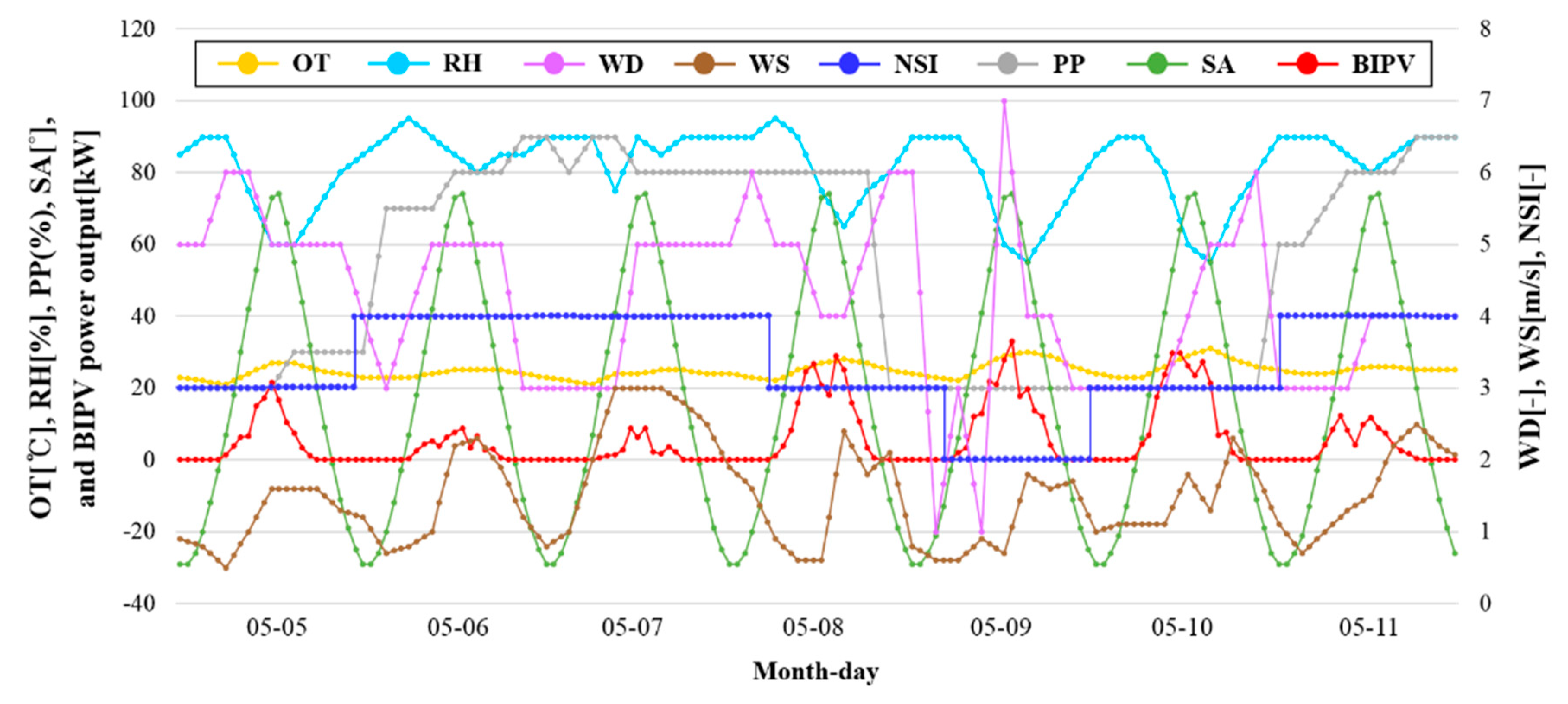
Although NSI indicates clearness of the sky, it was the least important factor with a variable importance score of 0.01 in clear and slightly cloudy days and 0.00 in cloudy and overcast days. This is mainly because of the characteristics of NSI data. KMA provides the float numbers for OT, RH, WS, and the degrees for WD (0~360) and SA (−90 ~ +90), whereas NSI has just four step integers: 1-no cloud, 2-intermittant cloud, 3-cloudy, and 4-overcast at intervals of 3 h with a geological resolution of 5 km by 5 km. As shown in Figure 5, as an example, the integer value of NSI is almost constant over a day, but the PV power output varies depending on the time and the SA. This illustrates the reason for the low correlation between NSI and PV power outputs. This feature plays a role in increasing the complexity of the prediction model and disrupts the prediction accuracy of the BIPV power output.

4. Model Selection

This section presents the proposed BIPV prediction model, which was used to compare six machine-learning models: ANN, SVM, CART, CHAID, RF, and RNN.

The hourly error of the prediction models was compared for evaluating model performance by the coefficient of variation of the root mean square error (CV(RMSE)), the mean absolute deviation (MAD), and the mean absolute percentage error (MAPE). Each index was calculated using the following equations.

$$\mathrm{CV}\left(\mathrm{RMSE}\right)=\frac{\sqrt{\frac{1}{n}{{\displaystyle \sum }}_{i=1}^n{(A_i-P_i)}^2}}{\overline{A_i}}$$

(4)

$$\mathrm{MAD}=\frac{1}{n}{\displaystyle \sum }_{i=1}^n\left|A_i-P_i\right|$$

(5)

$$\mathrm{MAPE}=\frac{1}{n}{\displaystyle \sum }_{i=1}^n\left|\frac{A_i-P_i}{A_i}\right|\times 100(\%)$$

(6)

where $n$ is the number of data values, $A_i$ is the actual BIPV power output, and $P_i$ is the predicted value of the BIPV power outputs.

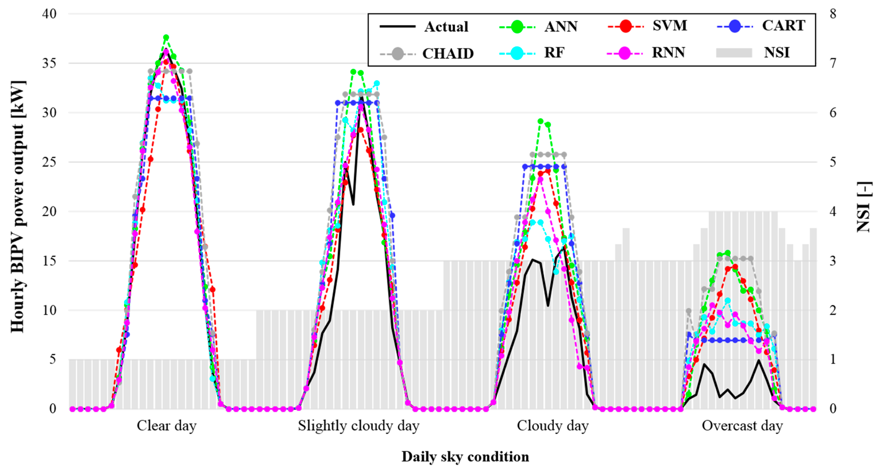
Figure 6 shows the results of the hourly BIPV predictions obtained using the six different machine-learning models with the four types of typical daily sky conditions. The results for each model show that the RNN outperformed the other models with an average hourly MAPE of 48.68% for four days, followed by RF (MAPE = 61.88%), CART (MAPE = 62.17%), SVM (MAPE = 66.63%), ANN (MAPE = 70.93%), and CHAID (MAPE = 98.52%).

Table 4. Comparison of model performance in terms of BIPV power output (64 days) for four types of sky conditions.

Days	Index	Prediction Models
		ANN	SVM	CART	CHAID	RF	RNN
Clear days (15 days)	CV(RMSE)	0.18	0.39	0.30	0.30	0.22	0.16
	MAD	1.18	2.69	1.98	2.02	1.54	0.80
	MAPE(%)	8.90	28.66	17.47	15.53	10.71	6.89
Slightly cloudy days (14 days)	CV(RMSE)	0.29	0.49	0.36	0.35	0.27	0.24
	MAD	1.85	3.06	2.02	2.16	1.65	1.44
	MAPE(%)	13.55	24.62	18.53	19.23	13.87	12.02
Cloudy days (17 days)	CV(RMSE)	0.77	0.72	0.90	0.91	0.86	0.41
	MAD	2.75	2.73	3.17	3.28	3.02	1.47
	MAPE(%)	32.45	35.12	43.88	42.87	34.60	19.21
Overcast days (18 days)	CV(RMSE)	1.60	1.57	1.32	2.12	1.46	1.10
	MAD	2.46	2.48	2.50	3.10	2.40	1.77
	MAPE(%)	71.28	63.41	72.11	99.48	66.85	51.34
Mean (64 days)	CV(RMSE)	0.76	0.83	0.76	0.98	0.75	0.51
	MAD	2.10	2.72	2.45	2.69	2.20	1.39
	MAPE(%)	33.72	39.27	40.08	47.21	33.54	23.79

lists the average hourly CV(RMSE), MAD, and MAPE of each machine-learning model for prediction for 64 days from May 2018 to August 2018 without missing data. By using the original weather forecast data set, the prediction performance was different for each model. In addition, all models had better prediction performance on clear and slightly cloudy days than on cloudy and overcast days. The RNN had the lowest average hourly error at 0.51, 1.39, 23.79% of CV(RMSE), MAD, and MAPE, respectively, for all periods.

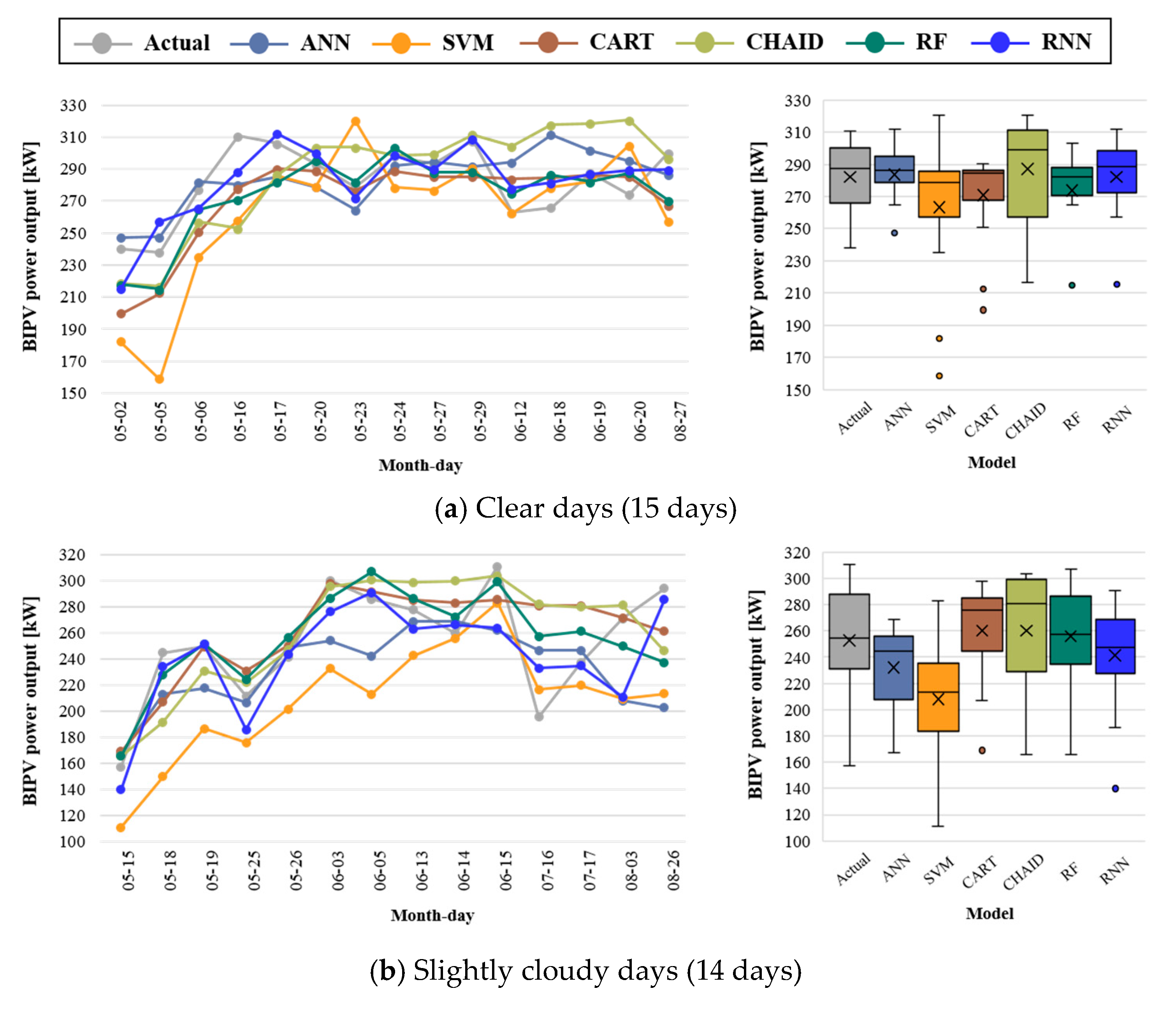
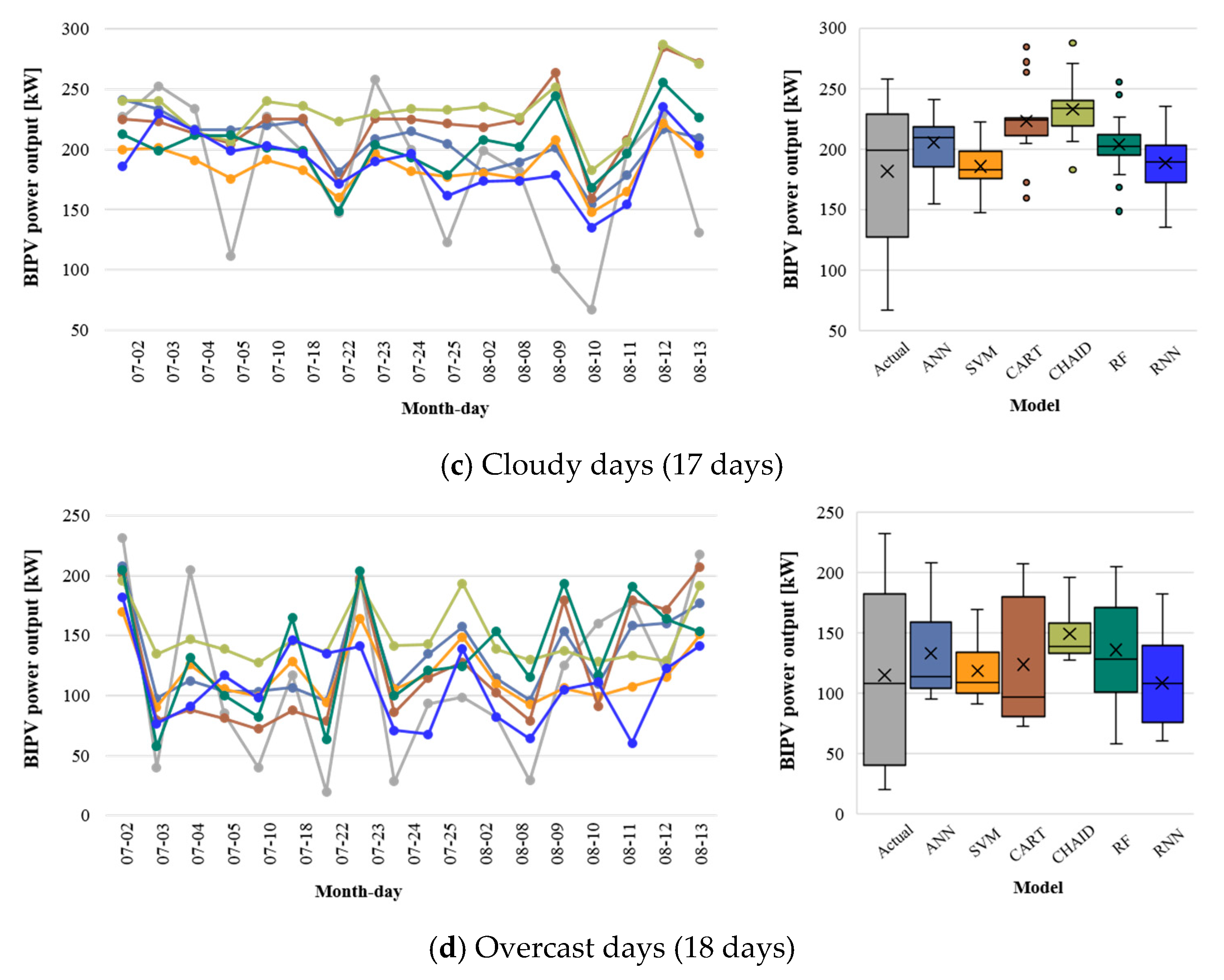
Figure 7 illustrates the daily PV power output (left) by summation of hourly actual measurements and model predictions. The means and deviations of daily total PV power output (right) varied depending on sky conditions and the model. The difference in the actual daily total PV output was 72.7 kW, 153.41 kW, 191.44 kW, 211.78 kW in clear, slightly cloudy, cloudy, and overcast sky conditions, respectively. The standard deviation ranged from 22.10 (clear) to 68.74 (overcast). All models performed better on clear and slightly cloudy days than on cloudy and overcast days, which was similar to the hourly prediction results. The large variance in PV power output on cloudy and overcast days affected the model performance.

As shown in Figure 7, the RNN outperformed the other models in estimating the daily total PV power output for the period. Although RNN predicted the hourly BIPV power output with less than 10% of MAPE and 0.20 of CV(RMSE) on clear and slightly cloudy days, the prediction performance decreased on cloudy and overcast days. In particular, the MAPE value of the daily total power output was higher than 50% on overcast days, which was similar to the values for the other models. This may imply that the prediction performance for overcast sky conditions does not depend on the model but, rather, the correlation between the input feature and the BIPV power generation.

Section 5 presents an investigation of the weather features that affect the hourly BIPV prediction performance on overcast days. Subsequently, this study proposes using the RNN with feature engineering, which can improve the prediction accuracy on overcast days.

5. Performance Improvement by Dropout Observation

This section presents techniques to improve the BIPV prediction performance on overcast days by using the feature engineering method based on the RNN model.

5.1. Effect of Dropout Observation

The variable importance indicated that the NSI is a redundant variable that contains high levels of noise, which prevents accurate predictions.

Section 4 demonstrated that the RNN is the most promising model but its performance on the 18 overcast days was not good as the clear or slightly cloudy days. In general, the NSI was 4 for the entire day on overcast days but the hourly BIPV output fluctuated with time, as shown in Figure 5. In addition, on several days, the onsite weather was clear, but the weather forecast was overcast or vice-versa.

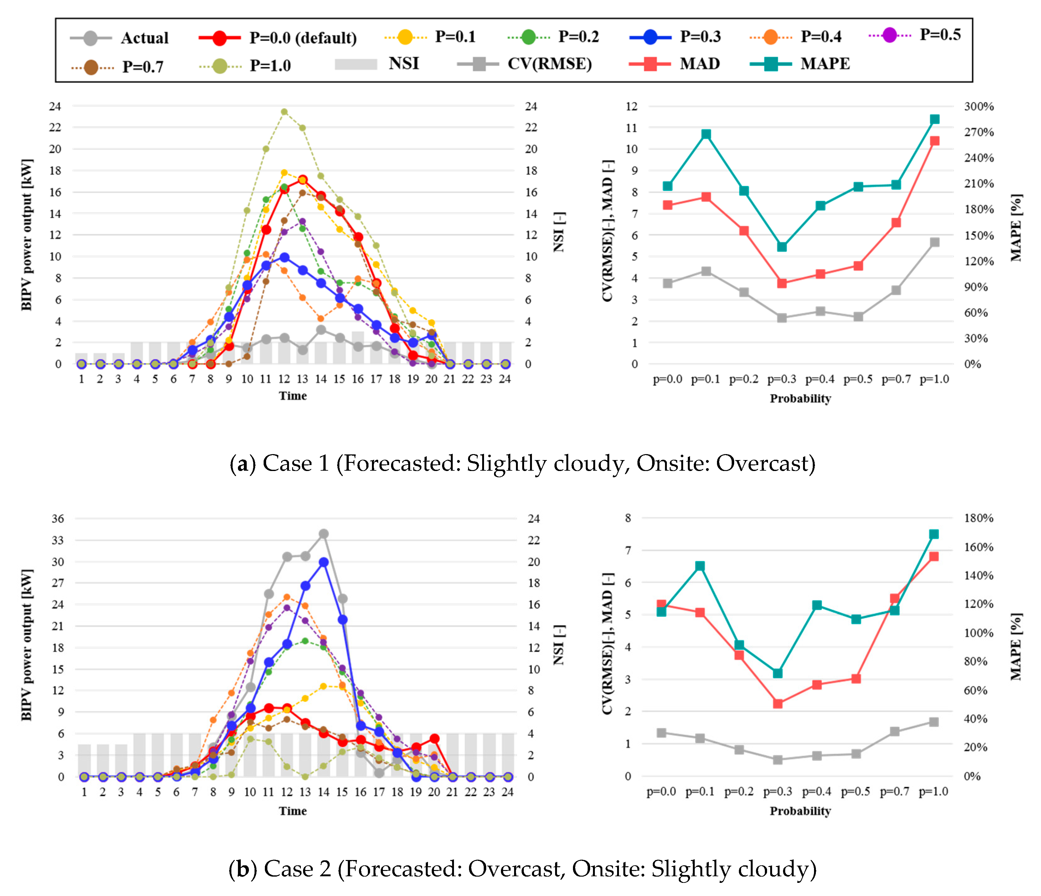
Figure 8 shows the results of the hourly BIPV power prediction on overcast days combined with different levels of observation dropout using RNN. In Figure 8a, the onsite weather was overcast but the NSI was 2 (slightly cloudy) for the entire day. In the other (Figure 8b) case, the onsite weather was slightly cloudy, whereas the NSI was 4, i.e., overcast. The hourly average MAPE varied by different values of p. The prediction results of p = 0.0 (without the dropout observation) and that of p = 1.0 (without all the NSI data for the training and predicting process) illustrates that the dropout observation is necessary to improve the prediction performance. The hourly predicted value, at a probability of 0.3, was closer to the actual BIPV power output than for the other probability variations.

The average hourly CV(RMSE), MAD, and MAPE on a day when both cases occurred was 2.54, 6.35, and 160.53%, respectively, with exposure to the default condition, but with a p of 0.3, the hourly prediction result of the BIPV power provided a more accurate fitting at 1.33, 3.00, and 103.52%, respectively. In particular, the hourly performance during the peak period from 11 a.m. to 3 p.m. was significantly better in all cases.

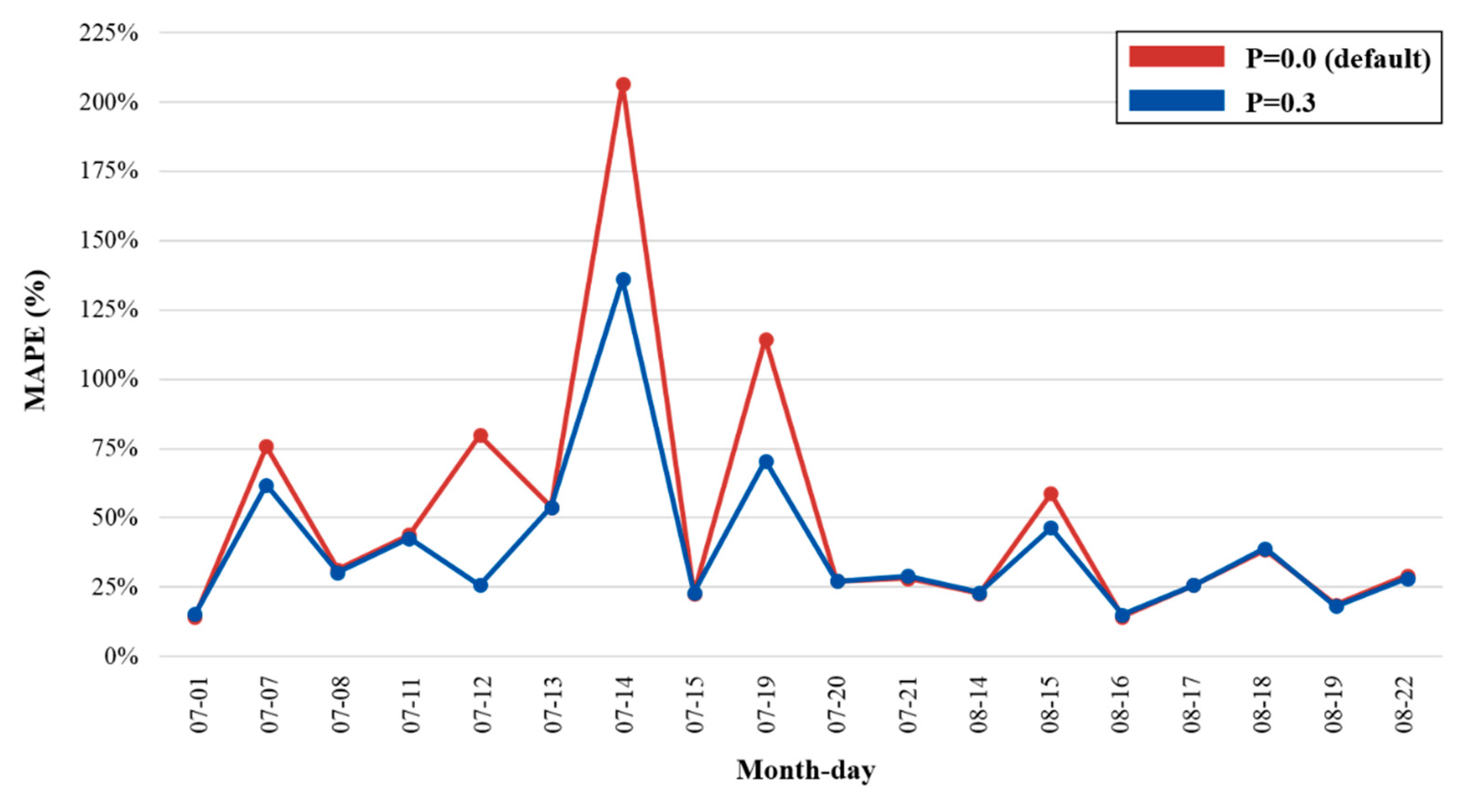
The daily predictions of the BIPV power validate the daily effect of the dropout observation at a p of 0.3 on 18 overcast days. Figure 9 compares the average hourly MAPE on a day characterized by the best-performing p probability (= 0.3) and the original RNN at p = 0.0 over the same period. The effect of the dropout observation provides a more optimal fit for the 5 days during which the unstable weather conditions prevailed. The average hourly MAPE per day at p = 0.3 was 68.16%, compared with the MAPE for the default condition, which was 107.13% for 5 days. For 18 days, the daily prediction performance with the dropout observation produced a minimum MAPE of 39.67%, which was an improvement on the performance compared with the original configuration of 50.48% MAPE. Therefore, the dropout observation method improves the hourly prediction accuracy of the RNN model by more than 20% for overcast sky conditions, when the forecasted weather differs from the onsite weather.

5.2. Application and Integration of the Feature Engineered RNN Model

Direct models can predict BIPV power output with a simple environment that has historical PV power outputs and weather forecasted data. However, the prediction performance of the direct model depends on the accuracy of forecasted weather data. This study presents a machine-learning model, RNN with feature engineering, to include the benefits and reduce the drawbacks of the direct model approach. By feature engineering, the prediction performance of the model has been improved on cloudy and overcast days, in which the model accuracy decreases because of the high uncertainty of the sky condition as described in earlier sections.

The simple structure of the proposed model using an online weather forecasting service enables us to predict the hourly power outputs for the onsite BIPV without the substantial sensor network or data management system, which are not applicable for small or micro distributed energy resources (DER). This helps a building energy manager balance the supply and demand of electricity for the building and make a strategy for purchasing electricity from the grid.

In addition, the aggregators for DERs in the smart grid, virtual power plant, or energy cloud can simply estimate the hourly PV power output of several DERs in a day-ahead. This allows the smart grid operators make an optimal decision on whether the generated power should be traded into the electricity market or be stored, to maximize the efficiency of the BIPV application and the benefits of the electricity storage system.

6. Conclusions

The short-term BIPV power output prediction method is essential not only to manage the hourly electricity energy balance in a building but also to transfer the generated power from the BIPV into the grid. Although the indirect method can yield a higher prediction accuracy depending on the prediction accuracy of the solar radiation, it requires solar radiation data, DNI or GHI at a particular site. However, the direct method is able to predict the PV power output with conventional forecasted weather data, not including solar irradiation, but the accuracy depends on differences between the forecasted and actual on-site weather conditions.

This study introduced a novel approach to improve the prediction performance of the short-term BIPV power output with a direct method using feature engineering and machine learning. Feature selection (based on variable importance with SVM) was used with seven variables from the weather forecast data to identify the factor that prevents improvements in short-term BIPV power prediction. Among the forecasted weather variables, NSI has the lowest correlation scores to the PV power output in most sky conditions because of the variable characteristics from the weather forecast service. NSI proved to be redundant for the training and prediction process.

Six machine-learning algorithms, namely the ANN, SVM, CART, CHAID, RF, and RNN algorithms, were compared to identify an appropriate prediction model using historical weather data exposed to four typical types of weather conditions. The results demonstrated that the RNN provides the best predictive performance. The RNN outperformed the other methods not only in terms of hourly predictive accuracy but also with regard to long-term daily prediction performance for 64 days. Although the RNN exhibited high accuracy on clear and slightly cloudy days, the prediction performance on overcast days was higher than 50% of the average hourly MAPE.

Dropout observation with different probabilities of NSI, the lowest correlated variables, was then applied to the RNN model training and predictions to remove additional noise in the neural net for PV power output prediction on overcast days. The results showed that the prediction performance improved by more than 20% compared with the RNN for 18 overcast days without feature engineering. Therefore, the observation dropout of the feature engineering method appears to be capable of providing reliable prediction performance for both hourly intervals and daily BIPV power output for short-term periods.

Although we suggested a new approach to improve the hourly prediction performance of BIPV power output with the direct method, this study has room for improvement with respect to investigating the prediction performance with different model configurations, different variables for dropout observation, and input levels. It is necessary to optimize the short-term trade schedule for the predicted PV power output into the grid, one day ahead, in the microgrid. This can be used to minimize the purchased electricity from the grid by incorporation into the energy storage system (ESS).