A New Improved Voltage Stability Assessment Index-centered Integrated Planning Approach for Multiple Asset Placement in Mesh Distribution Systems

Abstract

This paper offers a new improved voltage stability assessment index (VSAI_B)-centered planning approach, aiming at the attainment of technical and cost related objectives with simultaneous multiple asset deployment in a mesh distribution systems (MDS). The assets such as multiple distributed generation (DG) and distributed static compensator (D-STATCOM) units have been utilized; aiming at voltage stabilization, loss minimization, and associated objectives. The proposed planning approach incorporates expressions of VSAI_B aiming at initial simultaneous assets placement followed by loss minimization conditions (LMC) for appropriate asset sizing, which is further utilized for performance evaluations. The VSAI_B-LMC-based integrated planning approach is applied to configured MDS models such as a 33-bus test distribution system (TDS) for detailed analysis. The performance evaluations with the presented approach have been conducted for different cases along with respective scenarios considering various technical and cost-economic performance metrics. First, three cases referring to multiple DGs sitting and sizing for various power factors have been presented, followed later by two cases of multiple DGs and D-STATCOMs with respective evaluation scenarios. Finally, benchmark analysis is conducted on a 69-bus TDS for validity demonstration of the proposed approach. The comparison of achieved results in comparison with the available literature points out toward the validity and improved performance of the proposed approach.

1. Introduction

The distribution system (DS) under the traditional grid paradigm was deterministically designed for unidirectional power flow operation from substations towards the endpoints under a radial topology [1]. However, increasing load, population growth, large scale urbanization, and power quality concerns have resulted in issues such as voltage instability and increased system losses, particularly at the distribution side of the grid. The replication of traditional planning tools and practices to reinforce DS with efficient asset management have neither remained feasible nor economically viable, which affects the hierarchal structure of the power grid [2].

The DS on the basis of topology is classified in terms of radial and interconnected (ring/loop/mesh) structures [3]. Most of the tools designed, methodologies formulated and associated strategies in the literature have been carried out for DS with radial topology and respective assets optimization as a prominent research paradigm [4]. From the DS planning (DS-P) viewpoint aiming at topology alteration, the tools designed for radial (topology-based) distribution systems (RDS) have limitations in terms of applicability for anticipated interconnected DS. Also, traditional methods have limitations in encompassing all the prerequisites for new planning methodologies in interconnected DS [4,5,6].

The future active distribution systems (ADS) are envisioned as a reliable (interconnected), efficient and sustainability-oriented feasible option under the smart grid (SG) paradigm [6]. The distributed generation (DG) units of various types are among with the key research focuses from the viewpoint of improving system performance, market deregulation and sustainability, primarily at the DS level. From the planning perspective, DG (including renewables) placement alongside other efficient devices, has a pivotal role in the modernization of current DS into ADS and meeting the limitations in their traditional counterparts [5]. However, asset optimization with DG integration or component reinforcement with traditional planning methodologies, may lead to serious challenges and technical issues rather than solution, particularly in the case of interconnected ADS [5,6].

Modernization of distribution grids along with DG utilization as planning options are among key research dimensions amongst researchers across the globe. These researchers have come up with numerous methodologies, techniques, and strategies which aim at optimal performance and efficient asset management of the DS with DGs and related devices. Moreover, the SG concept has enabled the realization of the concepts that were limited under the traditional paradigm [6]. Several efforts have put forward to address DS-P problems from various aspects. Moreover, the traditional DS-P has seen a transformation towards ADS planning, considering an increased level of complexity with asset optimization resulting in a feasible solution encapsulating all the economic, environmental and technical aspects. Optimization-based ADS planning has attracted researchers’ attention and efforts have put forward towards numerous techniques, models and tools to achieve asset management (predominantly DG) with the aimed objectives [4,5,6,7,8].

A literature review indicates numerous noteworthy research works that aim at DS-P with various asset reinforcements and achievement of goals with different methodologies. DG-oriented planning in DS as a core focus, has been reviewed from the perspectives of key factors, aids, optimization techniques, variables, objectives, constraints, models, challenges, modifications, methodology comparisons, and future trends [4,9,10,11]. In most of the aforementioned review works, DG-based planning (DG-P) and other asset optimizations consider the radial topology as a problem constraint. The DS-P in the reviewed literature has been addressed on the basis of single and multi-objective attainment within defined constraints, aiming at global or trade-off solutions. Moreover, a methodology for the concerned DS-P is usually assessed on the basis of the genre of technique, suitability, limitations, time, computation, complications and complexity, respectively. Noteworthy DS-P asset optimization problems aim at encapsulating analytical methods, numerical techniques, meta-heuristics (MH) approaches, artificial intelligence (AI)-based algorithms, and hybrids of the mentioned techniques in various stages and different methodologies, respectively [12,13]. Hence, DS_P with interconnected ADS, needs to be investigated with an efficient technique.

On the basis of a relative comparison from viewpoint of DS-P methodologies, the conventional techniques (analytical, numerical, etc.) have been widely used for optimal DG placement (ODGP) problem focusing RDS as test systems [14,15]. These conventional techniques need comparatively high computation and focus usually at the attainment of loss minimization (LM). However, they are usually based on mathematical formulations and encapsulate the dynamics of a DS in an equivalent model. Also, improved variants of these techniques result in better utilization in terms of ODGP problems, as discussed in [15,16,17]. Since most conventional techniques have numerical relationships formulated considering two buses (one branch) equivalent models aiming at RDS [18], the modified variants considering interconnected DS with respective equivalent models are research-worthy issues. Nature and other processes inspired intelligent algorithms (meta-heuristics, artificial intelligence, etc.) have addressed the complexity in multi-dimensional DS-P problems [4,5,8,19]. However, they are liable to find a local solution rather than a global one, due to premature termination and search space issues with random initialization. Also, the computation time increases with a slow convergence. The hybrid methods address issues in the aforementioned algorithms [4,5,8]. However, they need fine tuning of concerned parameters and complications in the coding process is still a technical issue, as presented in [13,14,19,20,21,22,23,24]. Thus, an improved planning methodology, ignoring radial constraints with reduced search space, needs to be further explored.

Besides DS-P based on the aforementioned works considering RDS as test DS, a considerable amount of research work is available in the literature based on ignoring the radial structure constraint aiming at interconnected topologies such as loop and mesh topologies in DS. The feasibility studies for upgrading the topology from RDS to loop distribution systems (LDS), is discussed under various performance metrics [3,6]. An existing RDS can be converted into LDS by closing the most optimal normally open tie-switch (TS) or to MDS via a selection of multiple TS. The basic theory of interconnected DS is the same, provided, short circuit levels, improved protection schemes, and concerned issues have been considered during planning, enhancement and modernization phase, respectively. Such plans are more suitable for urban areas, which are densely populated and result in cost-effective feasible solutions with the utilization of existing infrastructure [25].

LDS has been assessed from the planning of DGs, with a sensitivity and non-dominated sorting genetic algorithm II-based approach in [26] and a graph-partitioning-integer-programming method for efficiency and reliability in [27,28]. Moreover, LDS planning with multiple DGs has been assessed with integrated voltage stability index (VSI) and loss minimization condition (LMC) across load growth with performance evaluations, as reported in [29]. An economic analysis-based study to upgrade RDS to LDS, with optimal number and location of fault current limiters (FCL) is presented in [30], which aims at finding a trade-off feasible solution considering reliability and system losses minimization. An in-depth LM approach centered towards circuit theory is proposed for interconnected ADS [31].

MDS on the other hand, is also assessed in the literature from a planning perspective of a futuristic model of ADS under the SG paradigm. A framework envisaging multiple-objective attainment-based optimization is offered to upgrade the LDS into MDS with respective performance analysis [32]. MDS is also evaluated under various load levels and load growth phenomenon without DGs, as demonstrated in [33]. A comparative study with evaluation of four methods in MDS with the goal to increase DG penetration was proposed in [34], and is conducted by replacing the TS with FCL. An enhanced voltage stability assessment index (VSAI) and LMC-based approach is proposed to address order-wise and multiple DG units’ placement under various power factors (PF), and evaluated under different performance indices in MDS under normal load level, respectively [35].

Moreover, the application of planning with optimal sitting and sizing of distributed static compensators (D-STATCOMs) with DGs have been mostly conducted for RDS, as mentioned in reviewed works [36]. It is indicated in the reviewed work that various methodologies used to solve the aforementioned problem aim towards the achievement of power losses mitigation, improvement in voltage profile and reduction in associated costs. Most of the concerned works have been applied to RDS under various load levels as test systems and the methodologies employed cannot comprehend the actual interconnected system. Although, a few works have considered DG with D-STATCOM (DSt) placement in MDS. Gupta et al. [37] have evaluated DSt placement with various VSI-based sensitivity approaches, initially formulated for RDS. The concerned VSIs were based on two bus and single branch equivalent DS and cannot encompass all the dynamics of LDS or MDS.

Similarly, Murty et al. [38] have evaluated DSt placement only with different load levels in various performance evaluations. Tolabi et al. [39] has proposed hybrid fuzzy-ant colony optimization and supported different buses for DG and DSt placements. The authors in [40] consider a bacterial foraging optimization algorithm for multiple DG and DSt set placements on the same buses, and the contributions of active and reactive power components from each asset. Yuvaraj et al. in [41] have also emphasized placement of multiple sets of DG and DSt, on the same respective designated buses. Moreover, Devi et al. [42] has evaluated the impact of DG and DSt placements, on the same bus along with different locations, utilizing particle swarm optimization. Taher et al. [43] have evaluated the technical performance of DSt along with a respective cost analysis.

It is discussed that the magnitude of voltage alone is not a suitable measure for the voltage stability (VS) valuation of a DS [44]. Numerous VS-based indices are available in the literature that aim at optimizing the DG (site and size), with a few works considering DSt utilization, mostly within RDS, and few in MDS [18,36]. These related VS indexes are based on equivalent two bus and single branch models and are used to represent equivalent RDS models. In addition, from an application perspective, RDS-related voltage-based evaluation indicators do not apply to LDS and MDS. Similarly, a VSI based on a single-branch can show some limitations for LDS (two branches) and MDS (multi-branch) models alike [45]. In our previous publications, a dedicated VSI for LDS was proposed in [45] and employed with LMC in [29], using an integrated planning approach for normal and load growth under various cases for LM and voltage maximization (VM). The limitations of LDS-based VSI have bridged in [29] across MDS with an enhanced voltage stability assessment index (VSAI) with various performance evaluations under normal load, as offered in [35]. However, the resulting VSAI expressions become complex and require a comparatively large computation effort.

Moreover, few of the abovementioned works consider VSI based on an equivalent MDS model with simultaneous placements of multiple DG and multiple assets (DG + DSt) evaluating both technical and cost-related performance indices evaluations, such as VM, LM, cost reductions, respective DG and DSt penetrations, etc. Hence, the aim of this paper is to propose a new improved simplified expression for VSAI (referred to in this paper as VSAI_B) with LMC to bridge the aforementioned research gaps. The abovementioned limitations serve as the motivation for the proposed research efforts in this paper. Moreover, the enhanced performance evaluation besides technical parameters assessment considers cost as an important evaluation parameter.

This research paper offers an integrated VSAI_B-LMC approach, evaluated under various performance measures for the optimal sitting and sizing of multiple DGs and D-STATCOMs under various cases and their respective scenarios. The new VSAI_B covers the overall aspect of MDS and addresses the concerned limitations overlooked in previous publications for the required application. The most important aspect is that VSAI (referred to in this paper as VSAI_A) in [35] runs for two times for simultaneous DG placement and three times for order-wise variant for DG placement, besides for the base case, respectively. The proposed VSAI_B runs for the base case only and gives optimal locations for simultaneous placement of multiple DGs and assets (DG + DSt), and considerably reduces the search space for computation, respectively. The key contributions of the presented research work are as follows:

(i)

Improved mathematical expressions of VSAI_B based on an equivalent MDS circuit.

(ii)

Loss minimization condition (LMC) for an equivalent electrical MDS circuit.

(iii)

Integrated planning approach based on VSAI_B and LMC, for equivalent electrical MDS circuits.

(iv)

Simultaneous assets placement with a single run of the respective computation procedure.

(v)

Evaluation of the offered approach on a 33-bus test distribution system (TDS).

(vi)

Performance evaluation with multiple DGs (siting and sizing) under various PF.

(vii)

Performance evaluation of techno-economic objectives with multiple DGs only at various PF.

(viii)

Performance evaluation with multiple DGs and D-STATCOMs (DSt).

(ix)

Performance evaluation of techno-economic objectives with multiple DGs and DSt.

(x)

Performance evaluation of the proposed approach on a 69-bus TDS for benchmarking analysis.

(xi)

Validation of the proposed approach via comparison with results reported in the available literature.

This paper is arranged in the following order: Section 2 presents the complete mathematical derivations of the improved and simplified VSAI_B expression for MDN. Section 3 presents LMC expressions for both active and reactive components within MDS. The proposed VSAI_B-LMC-based improved integrated planning approach is demonstrated with computation procedures, assumptions, and constraints, indices for performance evaluation and simulation setups; as mentioned in Section 4. In Section 5, the proposed integrated planning approach is evaluated under different performance metrics, with multiple DGs operating at various PF followed by multiple assets (DGs and DSt) placements and demonstrated on a 33-bus TDS. A benchmark analysis is conducted on 69-bus TDS as a separate case. The comparison of the proposed work with the available literature for validation is offered in Section 6. In Section 7, the paper is concluded.

2. Improved Voltage Stability Assessment Index (VSAI_B) for Mesh Distribution System

The equivalent MDS model that corresponds to an electrical equivalent, consists of overall five branches. Three of the five branches are indicated as distribution feeders and the remaining two correspond to the tie-line branches (TB) connecting three main distribution branches together. When the respective tie-switches (TS) such as TS1 and TS2 are closed, the RDS system can be transformed into a multiple-loop configured MDS. The proposed VSAI from the viewpoint of an actual MDS electrical equivalent circuit model corresponds to an arrangement which assumes that the TB along with respective TS may have small impedance and can be safely ignored. Also, the three buses feeding the respective load are assumed at the same voltage levels and are represented as fed from three sources (at the same voltage) initiating from the substation (SS). These assumptions reduce the equivalent MDS model to a further simplified one, as shown in Figure 1. It is assumed that voltages (U) across sending end buses (SBs such as m_1b, m_3b, and m_5b) are the same, with zero difference of voltage (ΔU) and phase angle (δ).

The receiving end buses (RBs such as m_2b, m_4b and m_6b) are connected to each other with TB1 (with TS1 is between m_2b and m_4b) and TB2 (with TS2 is between m_2b and m_6b). All TBs are assumed to have negligible impedance and thus ignored. The loads on the RBs (S_2b, S_4b and S_6b) at the respective nodes are assumed as add up to a single lumped load at RE m_2b, as shown in Figure 1, respectively. The voltages at RBs (U_2b, U_4b and U_6b) are also considered at the same level and are represented with U_2b. The system shown in Figure 1 considers most of the aspects of an equivalent MDS. Also, the sending end (SE) nodes (m_1b, m_3b and m_5b) with respective voltages (U_1b, U_3b and U_5b) have been considered to be originated from same substation. The respective branch currents in each branch are designated by I_1B, I_2B and I_3B. The branch current in each distribution line can be evaluated from the following Equation (1), as follows:

$$I_{1B}={\left[\frac{P_{2b}+j{Q}_{2b}}{U_{2b}\angle {\delta }_{2b}}\right]}^{*}; I_{2B}={\left[\frac{P_{4b}+j{Q}_{4b}}{U_{4b}\angle {\delta }_{4b}}\right]}^{*}; I_{3B}={\left[\frac{P_{6b}+j{Q}_{6b}}{U_{6b}\angle {\delta }_{6b}}\right]}^{*}$$

(1)

Since, the voltage is assumed to be the same across all the receiving end nodes i.e.,$U_{2b}\angle {\mathsf{\delta }}_{2b}=U_{4b}\angle {\mathsf{\delta }}_{4b}=U_{6b}\angle {\mathsf{\delta }}_{6b}$, hence, node 2 designated by m_2b is considered as reference node with respective voltage to be $U_{2b}\angle {\mathsf{\delta }}_{2b}$. The Equation (2) can be rearranged and rewritten as follows:

$$I_{1B}={\left[\frac{P_{2b}+j{Q}_{2b}}{U_{2b}\angle {\delta }_{2b}}\right]}^{*}; I_{2B}={\left[\frac{P_{4b}+j{Q}_{4b}}{U_{2b}\angle {\delta }_{2b}}\right]}^{*}; I_{3B}={\left[\frac{P_{6b}+j{Q}_{6b}}{U_{2b}\angle {\delta }_{2b}}\right]}^{*}$$

(2)

The RB node/bus voltage can be written, as shown in Equation (3), considering it is fed from three source ends in MDS. Where Z₁, Z₂ and Z₃ are branch impedances:

$$U_{2b}\angle {\delta }_{2b}=U_{1b}\angle 0+ U_{3b}\angle 0+ U_{5b}\angle 0-\left[I_{1B}{Z}_{1 }\right]-\left[I_{2B}{Z}_{2 }\right]-\left[I_{3B}{Z}_{3 }\right]$$

(3)

Equation (3) can be expanded by including the current and impedance relationships:

$$\begin{gathered} U_{2b}\angle {\delta }_{2b}=U_{1b}\angle 0+ U_{3b}\angle 0+ U_{5b}\angle 0-{\left[\frac{P_{2b}+j{Q}_{2b}}{U_{2b}\angle {\delta }_{2b}}\right]}^{*}\left[R_{1r }+j{X}_{1x}\right] \\ -{\left[\frac{P_{4b}+j{Q}_{4b}}{U_{2b}\angle {\delta }_{2b}}\right]}^{*}\left[R_{2r }+j{X}_{2x}\right]-{\left[\frac{P_{6b}+j{Q}_{6b}}{U_{2b}\angle {\delta }_{2b}}\right]}^{*}\left[R_{3r }+j{X}_{3x}\right] \end{gathered}$$

(4)

By adjusting conjugate, the improved expression is as follows in Equation (5):

$$\begin{gathered} U_{2b}\angle {\delta }_{2b}=U_{1b}\angle 0+ U_{3b}\angle 0+ U_{5b}\angle 0-\left[\frac{P_{2b}-j{Q}_{2b}}{U_{2b}\angle -{\delta }_{2b}}\right]\left[R_{1r }+ j{X}_{1x}\right] \\ -\left[\frac{P_{4b}-j{Q}_{4b}}{U_{2b}\angle -{\delta }_{2b}}\right]\left[R_{2r }+ j{X}_{2x}\right]-\left[\frac{P_{6b}-j{Q}_{6b}}{U_{2b}\angle -{\delta }_{2b}}\right]\left[R_{3r }+ j{X}_{3x}\right] \end{gathered}$$

(5)

The expanded expression is shown in Equation (6) as follows:

$$\begin{array}{ll}{\left|U_{2b}\right|}^2=U_{1b}{U}_{2b}& \angle -{\delta }_{2b}+U_{3b}{U}_{2b}\angle -{\delta }_{2b}+U_{5b}{U}_{2b}\angle -{\delta }_{2b}\\ & -\left[abs\right\{(P_{2b}{R}_{1r }+ P_{4b}{R}_{2r }+ P_{6b}{R}_{3r })\\ & +(Q_{2b}{X}_{1x}+ Q_{4b}{X}_{2x}+ Q_{6b}{X}_{3x})\left\}\right]\\ & -j\left[abs\right\{(P_{2b}{X}_{1x}+ P_{4b}{X}_{2x}+ P_{6b}{X}_{3x})\\ & -(Q_{2b}{R}_{1r }+ Q_{4b}{R}_{2r }+ Q_{6b}{R}_{3r })\left\}\right]\end{array}$$

(6)

The real and imaginary parts of Equation (6) have separate and resulting relationships that are shown in Equations (7) and (8), respectively. It is significant to mention that the expression $\left[abs\left\{\left(P_{2b}{R}_{1r }+ P_{4b}{R}_{2r }+ P_{6b}{R}_{3r }\right)+\left(Q_{2b}{X}_{1x}+ Q_{4b}{X}_{2x}+ Q_{6b}{X}_{3x}\right)\right\}\right]$ of Equation (6), indicating real part is designated as A, whereas imaginary part of the same equation $\left[abs\left\{\left(P_{2b}{X}_{1x}+ P_{4b}{X}_{2x}+ P_{6b}{X}_{3x}\right)-\left(Q_{2b}{R}_{1r }+ Q_{4b}{R}_{2r }+ Q_{6b}{R}_{3r }\right)\right\}\right]$ is designated as B:

$${\left|U_{2b}\right|}^2+ A=U_{1b}{U}_{2b}cos\angle {\delta }_{2b}+U_{3b}{U}_{2b}cos\angle {\delta }_{2b}+U_{5b}{U}_{2b}cos\angle {\delta }_{2b}$$

(7)

$$B=- U_{1b}{U}_{2b}sin\angle {\delta }_{2b} - U_{3b}{U}_{2b}sin\angle {\delta }_{2b}- U_{5b}{U}_{2b}sin\angle {\delta }_{2b}$$

(8)

By squaring Equations (7) and (8), the modified expressions are indicated in Equations (9) and (10) as follows:

$$\begin{array}{ll}{\left|U_{2b}\right|}^4+ A^2+2A& {\left|U_{2b}\right|}^2\\ & =U_{1b}{}^2{U}_{2b}{}^2{cos}^2\angle {\delta }_{2b}\\ & +U_{3b}{}^2{U}_{2b}{}^2{cos}^2\angle {\delta }_{2b} +U_{5b}{}^2{U}_{2b}{}^2{cos}^2\angle {\delta }_{2b}+2U_{1b}{U}_{2b}\left(\frac{1+cos\angle 2{\delta }_{2b}}{2}\right)\\ & +2U_{3b}{U}_{2b}\left(\frac{1+cos\angle 2{\delta }_{2b}}{2}\right)+2U_{5b}{U}_{2b}\left(\frac{1+cos\angle 2{\delta }_{2b}}{2}\right)\end{array}$$

(9)

$$\begin{array}{ll}{B}^2=U_{1b}{}^2{U}_{2b}{}^2{sin}^2\angle {\delta }_{2b}& +U_{3b}{}^2{U}_{2b}{}^2{sin}^2\angle {\delta }_{2b}\\ & +U_{5b}{}^2{U}_{2b}{}^2{sin}^2\angle {\delta }_{2b}+2U_{1b}{U}_{2b}\left(\frac{1-cos\angle 2{\delta }_{2b}}{2}\right)\\ & +2U_{3b}{U}_{2b}\left(\frac{1-cos\angle 2{\delta }_{2b}}{2}\right)+2U_{5b}{U}_{2b}\left(\frac{1-cos\angle 2{\delta }_{2b}}{2}\right) \end{array}$$

(10)

After addition of Equations (9) and (10) and reduction by the use of the respective trigonometric properties, the modified expression shown in Equation (11) is obtained:

$${\left|U_{2b}\right|}^4+ A^2+B^2+2A{\left|U_{2b}\right|}^2= {\left|U_{2b}\right|}^2{\left|U_{1b}+U_{3b}+U_{5b}\right|}^2$$

(11)

The rearranged equation as per quadratic equation real root form b² − 4ac > 0, is indicated as follows.

$${\left|U_{2b}\right|}^4-\left[{\left|U_{1b}+U_{3b}+U_{5b}\right|}^2-2A\right] {\left|U_{2b}\right|}^2+ \left[A^2+B^2\right]\ge 0$$

(12)

The expansion and readjusted expression in Equation (12), point out a real root feasible solution only in terms of a real root (b² − 4ac > 0). Both sides of the equation are divided by $3^4:$

$$\frac{{\left|U_{1b}+U_{3b}+U_{5b}\right|}^4}{3^4}-4A\frac{\left[{\left|U_{1b}+U_{3b}+U_{5b}\right|}^2\right]}{3^4}-\frac{4 B^2}{3^4}\ge 0$$

(13)

Since a load bus in an actual MDS can be fed by two or more SE buses. Hence, the number of SE that are feeding a RB is considered as m_l = n = 3 (SE buses in MDS)

$$\frac{{\left|U_{1b}+U_{3b}+U_{5b}\right|}^4}{n^4}-\frac{4A}{n^2}\frac{\left[{\left|U_{1b}+U_{3b}+U_{5b}\right|}^2\right]}{n^2}-\frac{4 B^2}{n^4}\ge 0$$

(14)

In order to simplify the equation, the sum of all SE voltage magnitudes are represented as ${\displaystyle \sum }_{s=1}^{m_l}{\left(U_{sb}\right)}^4={\left(U_{1b}+U_{3b}+U_{5b}\right)}^4$ after division by $n^4$ nodes. The modified expression is shown in Equation (15) as follows:

$${\displaystyle \sum }_{s=1}^{m_l}{\left(\frac{U_{sb}}{n}\right)}^4-\frac{4A}{n^2}{\displaystyle \sum }_{s=1}^{m_l}{\left(\frac{U_{sb}}{n}\right)}^2-\frac{4 B^2}{n^4}\ge 0$$

(15)

After subsequent rearranging, the expression for scaled VSI is shown in Equation (16):

$$VSI= \frac{\frac{4}{n^2}\left[A{{\displaystyle \sum }}_{s=1}^{m_l}{\left(\frac{U_{sb}}{n}\right)}^2+ {\left(\frac{B}{n}\right)}^2\right]}{{{\displaystyle \sum }}_{s=1}^{m_l}{\left(\frac{U_{sb}}{n}\right)}^4} \le 1$$

(16)

In order to rescale the proposed VSI, the relationship shown in Equation (16) is multiplied by $n^4$:

$$VSIs=n^4\times VSI= n^4\times \frac{\frac{4}{n^2}\left[A{{\displaystyle \sum }}_{s=1}^{m_l}{\left(\frac{U_{sb}}{n}\right)}^2+ {\left(\frac{B}{n}\right)}^2\right]}{{{\displaystyle \sum }}_{s=1}^{m_l}{\left(\frac{U_{sb}}{n}\right)}^4}$$

(17)

The rescaled expression of VSIs or simply VSAI_B is illustrated in Equation (18). It is considered that under normal conditions, the numerical value of VSAI_B is close to zero even after scaling (multiplication by $n^4$) and the upper bound of stability remains equal to 1. During unstable conditions, the expression exceeds numerical threshold of 1:

$$VSAI\_B= VSIs= 4n^2\frac{\left[A{{\displaystyle \sum }}_{s=1}^{m_l}{\left(\frac{U_{sb}}{n}\right)}^2+ {\left(\frac{B}{n}\right)}^2\right]}{{{\displaystyle \sum }}_{s=1}^{m_l}{\left(\frac{U_{sb}}{n}\right)}^4} \le 1$$

(18)

It is worth mentioning that under normal operating conditions, the numerical values associated with VSAI_B must be less than 1. Otherwise, the index shows vulnerability above 1. The VSAI_B limits described here apply only to the proposed index, other indices may have their respective proposed bounds. The voltage at receiving end is shown in Equation (19) and is indicated by V_B (U_2b) at bus m_2b. After substitution of scaled values of b =$\left[{\displaystyle \sum }_{i=1}^{m_l}{\left(\frac{U_{sb}}{n}\right)}^2-\frac{2A}{n}\right]$ and c from Equation (15), this results in Equation (19), which refers to a sub root indicating viable voltage solution:

$$V\_B = \left|U_{2b}\right| = \frac{1}{\sqrt{2}}\sqrt{\left[{\displaystyle \sum }_{s=1}^{m_l}{\left(\frac{U_{sb}}{n}\right)}^2-\frac{2A}{n}\right]+\sqrt{{\displaystyle \sum }_{s=1}^{m_l}{\left(\frac{U_{sb}}{n}\right)}^4-\frac{4A}{n^2}{\displaystyle \sum }_{s=1}^{m_l}{\left(\frac{U_{sb}}{n}\right)}^2-\frac{4 B^2}{n^4}}}$$

(19)

3. Loss Minimization Condition (LMC) in Mesh Distribution System

The impedance related with each distribution branch in electrical equivalent MDS model is denoted by $Z$_kB = R_kB + jX_kB (where k = 1, 2, 3), the corresponding resistance (R_k) and reactance (X_k). Likewise, the MDS equivalent model is considered to be equipped with three SB (U_1b, U_3b, and U_5b) and three RB (U_2b, U_4b, and U_6b) voltages, to fully cover all aspects a MDS model as shown in the Figure 2a. The loop currents circulating around connected branches and tie-branch (TB) in MDS needs to be simplified.

Mathematical expressions are required to simplify the loss equation and consider some assumptions in the equivalent MDS model. The TB parameters are negligible and all loads are concentrated as a single load, which can be supported by the negligible voltage difference across receiving buses (U_2b = U_4b = U_6b) as per assumption.

It is also considered that all sending end busses (SBs) are at same voltage level (U_1b = U_3b = U_5b) and can be concentrated to one source such as U_1b. The branch currents (I_1B, I_2B and I_3B) and respective circulating loop currents (designated with I_Lp1 and I_Lp2) among concerned feeders in distribution branch within the equivalent MDS model is shown in Figure 2a and expressed in Equation (20), which corresponds to an equivalent MDS model without DG unit inclusion. The direction of I_Lp1 (counter-clock-wise in direction) among branch 1 (m_1b to m_2b) and branch 2 (m_3b to m_4b), whereas I_Lp2 (clock-wise in direction) circulates between branch 2 (m_3b and m_4b) and branch 3 (m_5b and m_6b), respectively.

$$I_{Lp1}^{B2}= I_{2B} + I_{TB1}; I_{Lp1,2}^{B1}= I_{1B} + I_{TB1}+ I_{TB2}; I_{L2}^{B3}= I_{3B} + I_{TB2}$$

(20)

The relationships for branch and loop currents for base case considering LMC without DG inclusion, as illustrated in Figure 2a, are shown in Equations (21) and (22); respectively.

$$\begin{gathered} I_{2B}= I_{Lp1}^{B2}= \frac{1}{Z_{2B}+ \frac{Z_{1B}{Z}_{3B}}{Z_{1B}+Z_{3B}}}\left[\frac{Z_{1B}{Z}_{3B}}{Z_{1B}+Z_{3B}} I_{L{D}_A}\right] \\ {I}_{1B}=I_{Lp1,2}^{B1}= - \frac{1}{Z_{1B}+ \frac{Z_{2B}{Z}_{3B}}{Z_{2B}+Z_{3B}}}\left[\frac{Z_{2B}{Z}_{3B}}{Z_{2B}+Z_{3B}} I_{L{D}_A}\right] \\ {I}_{3B}=I_{Lp2}^{B3}= - \frac{1}{Z_{3B}+ \frac{Z_{1B}{Z}_{2B}}{Z_{1B}+Z_{2B}}}\left[\frac{Z_{1B}{Z}_{2B}}{Z_{1B}+Z_{2B}} I_{LD\_A}\right] \end{gathered}$$

(21)

$$I_{Lp1}= \left[\frac{-\left(U_{2b}+U_{4b}\right)+\left\{\frac{z_{1B}}{z_{1B}+z_{3B}}\left(U_{2b}+U_{6b}\right)\right\}}{\left\{z_{2B}+ \frac{z_{1B}{z}_{3B}}{z_{1B}+z_{3B}}\right\}}\right];I_{Lp2}= \left[\frac{\left\{\frac{z_{1B}}{z_{1B}+z_{2B}}\left(U_{2b}+U_{4b}\right)\right\}-\left(U_{2b}+U_{6b}\right)}{\left\{z_{3B}+ \frac{z_{1B}{z}_{2B}}{z_{1B}+z_{2B}}\right\}}\right]$$

(22)

The relationships for branch and loop currents after inclusion of DG unit for achievement of LMC is shown in Equations (23) and (24) and demonstrated in Figure 2b, respectively. It is assumed that with the deployment of optimal sizing of DG units, loop currents (I_Lp1 and I_Lp2) are reduced near to zero:

$$\begin{gathered} I_{2B}{}^{\prime }=I_{Lp1}^{B2}{}^{\prime }=\frac{1}{Z_{2B}+ \frac{Z_{1B}{Z}_{3B}}{Z_{1B}+Z_{3B}}}\left[\frac{Z_{1B}{Z}_{3B}}{Z_{1B}+Z_{3B}} \left(I_{LD\_A}-I_{DG\_A}\right)\right]\ge 0 \\ {I}_{1B}{}^{\prime }=I_{Lp1,2}^{B1}{}^{\prime }= - \frac{1}{Z_{1B}+ \frac{Z_{2B}{Z}_{3B}}{Z_{2B}+Z_{3B}}}\left[\frac{Z_{2B}{Z}_{3B}}{Z_{2B}+Z_{3B}} \left(I_{LD\_A}-I_{DG\_A}\right)\right]\ge 0 \\ {I}_{3B}{}^{\prime }=I_{Lp2}^{B3}{}^{\prime }= - \frac{1}{Z_{3B}+ \frac{Z_{1B}{Z}_{2B}}{Z_{1B}+Z_{2B}}}\left[\frac{Z_{1B}{Z}_{2B}}{Z_{1B}+Z_{2B}} \left(I_{LD\_A}-I_{DG\_A}\right)\right]\ge 0 \end{gathered}$$

(23)

The new LMC for apparent power (SLM) is shown in Equation (24):

$$SLM=\left[{\left(I_{2B}{}^{\prime }+ I_{Lp1}\right)}^2{Z}_{2B}+{\left(I_{1B}{}^{\prime }+ I_{Lp1}+ I_{Lp2}\right)}^2{Z}_{1B} + {\left(I_{3B}{}^{\prime }+ I_{Lp2}\right)}^2{Z}_{3B}\right]$$

(24)

The new LMC in the base case for active power (PLM) is shown in Equation (25):

$$\begin{gathered} PLM=[{\left(I_{2B\_P}{}^{\prime }+ I_{Lp1\_P}\right)}^2{R}_{2r}+{\left(I_{1B\_P}{}^{\prime }+ I_{Lp1\_P}+ I_{Lp2\_P}\right)}^2{R}_{1r} \\ + {\left(I_{3B\_P}{}^{\prime }+ I_{Lp2\_P}\right)}^2{R}_{3r}] \end{gathered}$$

(25)

The new LMC after DG for active power (PLMC’) is shown in Equation (26):

$$PLM{C}^{\prime }=\left[{\left(I_{2B\_P}{}^{\prime }\right)}^2{R}_{2r}+{\left(I_{1B\_P}{}^{\prime }\right)}^2{R}_{1r} + {\left(I_{3B\_P}{}^{\prime }\right)}^2{R}_{3r} \right]\ge 0$$

(26)

The new LMC for reactive power (QLM) is shown in Equation (27):

$$\begin{gathered} QLM=\left[{\left(I_{2B\_Q}{}^{\prime }+ I_{Lp1\_Q}\right)}^2{X}_{2x}+{\left(I_{1B\_Q}{}^{\prime }+ I_{Lp1\_Q}+ I_{Lp2\_Q}\right)}^2{X}_{1x} \\ + {\left(I_{3B\_Q}{}^{\prime }+ I_{Lp2\_Q}\right)}^2{X}_{3x}\right] \end{gathered}$$

(27)

The new LMC after DG for reactive power (QLMC’) is shown in Equation (28):

$$QLM{C}^{\prime }=\left[{\left(I_{2B\_Q}{}^{\prime }\right)}^2{X}_{2x}+{\left(I_{1B\_Q}{}^{\prime }\right)}^2{X}_{1x} + {\left(I_{3B\_Q}{}^{\prime }\right)}^2{X}_{3x}\right]\ge 0$$

(28)

4. Proposed Improved Integrated Planning Approach

The power companies across the globe have a responsibility to maintain a suitable voltage profile within specified levels across all feeders serving the respective loads. The power factor (PF) is also maintained at the utility’s end. When the load difference among distribution branches is disturbed, the distribution grid may lead to increased system losses in various situations. The proposed VSAI_B-LMC-based integrated planning approach is proposed to evaluate prime technical and cost related planning objectives from the perspective of MDS. Therefore, the prime objective of the proposed approach is to find feasible planning solution, capable of achieving the maximum relevant goals in MDS. The planning approach has presented with computation procedure, assumptions, constraints, indicators for performance evaluation and simulation setups are presented in following subsections.

4.1. Computation Procedure

The computation procedure for the proposed VSAI_B-LMC-based integrated planning approach refers to the simultaneous placement of DG and associated asset units in the respective meshed configured TDS. Regardless of TDS, the respective PF associated with each DG unit has considered with a variation of ±3%:

Step 1:

Read system data for the multiple loops configured TDS configured to MDS.

Step 2:

Run the load (power) flow for test MDS without DG or any asset, at normal load level.

Step 3:

According to Equation (18); calculate the corresponding VSAI_B at each RB. Moreover, the respective voltage profile as a feasible solution V_B is achieved according to Equation (19).

Step 4:

Select the three buses with the highest numerical values of proposed VSAI_B, as prospective candidates for the simultaneous placement of assets such as DGs operating at various PFs.

Step 5:

Run load flows for the test MDS after placement of three DGs. Increase the size of each DG at the respective PF with a variation of ± 3% at a relevant bus to a voltage limit that is close to or equal to the 1.0 ± 0.5% per unit (P.U), considering voltage level at substation (SS) as reference.

Step 6:

Find out voltage difference across each TB among the three tied feeders. The sizing of DG at a feeder with the highest voltage value is reduced to minimize the tie currents among other tied feeders and vice versa. For example, (refer to Figure 1 and Figure 2) if U_2b > U_4b and U_2b > U_6b, then U_2b is decreased by decreasing the DG (or DG+D-STATCOM) capacity integrated at a respective bus of feeder 1 to achieve LMC. Similarly, if U_4b > U_2b and U_6b > U_2b, then U_4b and U_6b are decreased by decreasing the DG (or DG+D-STATCOM) capacity integrated at respective buses at feeders 2 and 3; in order to achieve LMC and so on.

Step 7:

Repeat the process until the respective VSAI_B trend, results in a voltage profile (V_B) with the least voltage difference across TB1 (U_2b to U_4b) and TB2 (U_4b and U_6b), LMC condition along with PLMC’ or QLMC’ or any of them is achieved. When the aforesaid conditions are achieved with the respective DG or other asset sizes, the solution is feasible from the viewpoint of three DGs (or assets) in MDS. The calculated voltage V_C in equivalent Matlab/Simulink model is also provided for comparison and to establish the credibility of the achieved feasible solution V_B via the proposed VSAI_B-LMC approach.

Step 8:

Evaluate the concerned technical and cost (economics)-related performance indices on the basis of Steps 1–7, as mentioned in Section 4.4 later in this paper. A simple numerical example for illustration of the computation procedure is shown in Appendix A.

4.2. Assumptions for the Proposed Planning Approach

The assumptions for our VSAI_B-LMC-based proposed planning approach for MDS are as follows:

• The overall protection at the substation (SS) is considered as upgraded.
• Test MDS is 3-phase balanced and can be designated with an equivalent single-line diagram.
• The thermal limits in all branches have considered at a numerical value of 5 MVA ± 5%.
• The maximum number of DGs for integration, is three.
• The maximum number of assets for integration on a single node/bus a set of two assets (DG + DSt).
• DG unit can be integrated on any load bus except a slack bus from the SS.
• It is anticipated that for LMC achievement with planning approaches, if the receiving end buses (RBs at nodes m_2b, m_4b and m_6b) across TBs have ideally zero voltage difference i.e., U(m_2b) = U(m_4b) = U(m_6b) such that no loop current (I_TL) flows through, i.e., in this case both I_Lp1 and I_Lp2 are zero. The numerical value of ΔU is considered as 1.0% such as convergence criteria in within 0.01.
• Normal loading conditions in TDS have considered in the proposed study, i.e., load model is constant power and single load level.
• The variation in voltage values has considered around ±1.0%.
• The variation in PF (lagging) has considered around of ±3.0% in this study.
• It is assumed that shunt-capacitor banks are loads and line-shunt capacitance is negligible.

4.3. Constraints

The following main constraints have been considered in this study [46,47,48].

4.3.1. Active and Reactive Power Balance

It is considered that active power contribution from substation (P_SS) and DG units (P_DG) must have a balance that is equal to active power load consumption (P_LD) along with associated active power losses (P_Loss) in TDS, as shown in Equation (29). Also, the solution must not result in reverse power flow [46,47]:

P_SS + P_DG = P_LD + P_Loss

(29)

Similarly the reactive power substation (Q_SS) and DG units (Q_DG) must be equal to the reactive power load consumption (Q_LD) along with concerned reactive power losses (Q_Loss) in TDS, as shown in Equation (30) [46,47]:

Q_SS + Q_DG = Q_LD + Q_Loss

(30)

4.3.2. Voltage Constraint

The magnitude of the voltage at each node/bus “m” in TDS must not exceed the specified limit of 0.95 P.U to 1.05 P.U in accordance with the IEC or IEEE standards. In this paper the maximum voltage limit is considered around 1.0 P.U ± 1% in accordance with substation as a reference, as shown in Equation (31) [46,47]:

0.95 ≤ Vm ≤ 1.05; m = 1, 2, 3, 4 … n

(31)

4.3.3. Operating Power Factor (PF) of DG Unit

The lagging PF of DG needs to be within limits and a variation of ± 3% is allowed in DGs operating at lagging PF, one of which corresponds to utility favored 0.9 PF and other is equal to that of TDS load such as 0.85 PF in 33-bus (and 0.82 PF for 69-bus). PF_DG,i value ranges from PF_DG,i,min → PF − 3% to PF_DG,i,max → PF + 3% [48]:

$$P{F}_{DG, i,min}\le P{F}_{DG,i}\le P{F}_{DG,i,max}$$

(32)

4.3.4. Active and Reactive Power Limit of DG

The DG capacity integrated at bus ‘m’ in both active and reactive power terms (P_DG and Q_DG) must not exceed the maximum value of power counterparts from substation (P_SS and Q_SS) as illustrated in Equations (33) and (34) [48]:

$$P_m{}^{Mix}\le P_m\text{≤}{P}_m{}^{Max}\mathrm{i}.\mathrm{e}.,0\le P_m\le P_{ss}$$

(33)

$$Q_m{}^{Mix}\le Q_m\le Q_m{}^{Max}\mathrm{i}.\mathrm{e}.,0\le Q_m\le Q_{ss}$$

(34)

4.4. Indices for Performance Evaluation

The primary purposed approach is to find the likely location for the DG or any asset placement and sizing, which have objectives to retain a proper voltage level, system losses minimization, and concerned technical and cost-related goals, respectively. The technical and cost-related performance indicators have been illustrated in the following Section 4.4.1 and Section 4.4.2, respectively. In both the following technical and cost-related performance indicators, the sign (↑) indicates maximization of the objective and the sign (↓) indicates the minimization of the concerned objective, respectively.

4.4.1. Performance Indices for Technical Evaluation (TPI or TP)

The technical performance indicators (TPI) or technical parameters (TP) with the concerned mathematical relationships, units and aimed objectives are listed in

Table 1. Technical-based performance indices (designated in this paper as TPIs or TPs).

S#:	Performance Indices [29,35]	Performance Indices Relationships	Units:	Objective:
1	Active Power Loss (PLoss)	PLoss$=PLM{C}^{\prime }$=$min {\displaystyle \sum }_{i=1}^{m_l-1}{P}_{Loss}{}^{TDS}$+${{\displaystyle \sum }}^{}{P}_{TB}$	KW	↓
2	Reactive Power Loss (QLoss)	QLoss$=QLM{C}^{\prime }$= min${\displaystyle \sum }_{i=1}^{m_l-1}{Q}_{Loss}{}^{TDS}$+${{\displaystyle \sum }}^{}{Q}_{TB}$	KVAR	↓
3	Active Power Loss Minimization (PLM)	$PLM=\left[\frac{P\_L_{No\_DG}-P\_L_{M\_DG}}{P\_L_{No\_DG}}\right]\times 100$	%	↑
4	Reactive Power Loss Minimization (QLM)	$QLM=\left[\frac{Q\_L_{No\_DG}-Q\_L_{M\_DG}}{Q\_L_{No\_DG}}\right]\times 100$	%	↑
5	DG Penetration by percentage (DGPP)	$DGPP= \left({\displaystyle {\displaystyle \sum }_{a=1}^M}{P}_{DG}/{\displaystyle {\displaystyle \sum }_{b=1}^N}{P}_{LD}\right)\times 100$	%	↑
6	Active Power Capacity Release from Substation (PSSR)	PSSR = PSS − PDG ≥ 0	KW	↓
7	Reactive Power Capacity Release from Substation (QSSR)	QSSR = QSS − QDG ≥ 0	KVAR	↓

. The relevant details regarding all mentioned TPIs (or TP) can be found with background details in our previous publications [29,35,46,47,48]. The terms TPI and TP have been used interchangeably throughout the paper, indicating performance evaluation of various cases and respective scenarios in the proposed approach.

4.4.2. Performance Indices for Cost-Economic Evaluation

The cost (economic-based) performance indicators (CPI) or cost (economic-based) parameters (CP) have been listed with the associated relationships, units and objectives in

Table 2. Cost-economic-based performance indices (designated in this paper as CPIs or CPs).

S#:	Performance Indices/Ref	Performance Indices Relationships	Units:	Objective:
1	Cost of active power loss (PLC) [29,35]	$PLC=\left[P\_L \times E_U\times T_Y \left(8760 hrs\right)\right]$	M$	↓
2	Active power loss saving (PLS) [35]	$PLS=\frac{PL{C}_{No\_DG}-PL{C}_{M\_DG}}{PL{C}_{No\_DG}}\times 100$	M$	↑
3	Cost of DG for PDG (CPDG) [46]	$C\left(P_{DG}\right)$= a ×$P_{DG}{}^2+b\times P_{DG}+c$ Where: a = 0, b = 20, c = 0.25	$/MWh	↓
4	Cost of DG for QDG (CQDG) [46]	$C\left(Q_{DG}\right)$= $\left[C\left(S_{DG\_M}\right)-C\left(\sqrt{\left(S_{DG\_M}{}^2-P_{DG}{}^2\right)}\right)\right]$× k Where: $S_{D{G}_M}=\frac{P_{D{G}_M}}{cos\theta }=\frac{1.1 \times P_{DG}}{cos\theta };$ $k=0.5-1$	$/MVArh	↓
5	Annual Investment Cost (AIC) $AIC\left(Million\frac{US\$}{Year}\right)$ [29,35]	${\displaystyle {\displaystyle \sum }_{k=1}^{M_{DG}}}A{F}_C\times C{U}_C\times DG{C}_{max}$ $\mathrm{Where}:A{F}_c=\frac{\left(\frac{Ct}{100}\right){\left(1+\frac{Ct}{100}\right)}^T}{{\left(1+\frac{Ct}{100}\right)}^T-1}$	M$	↓
6	Annual Cost of D-STATCOM (ACD) [37,43]	$I_C=\left[\frac{{\left(1+B\right)}^{nDS}\times B}{{\left(1+B\right)}^{nDS}-B}\right]$ Where: $I_C$= 50$/KVAR; B = Rate of return of Assets = 0.1; nDS = 5 Years	M$	↓

.

The relevant details of the cost of active power loss (PLC), savings (PLS) and annual investment cost (AIC) can be found in our previous publications [29,35]. The cost of active (CPDG) and reactive power (CQDG) from DG can be found in [29,35,46,48] and an annual cost of D-STATCOM (DSt) can be found in [37,43]. The terms CPIs or CPs have been used interchangeably throughout the paper like their technical counterparts and indicate the performance evaluation of the proposed approach based on cost-related aimed objectives.

4.4.3. Types of DG in Performance Evaluation

There are three various type of DGs employed in this paper and the respective classifications from various performance metrics, particularly from the perspective of type, PF, sizing, and cost of DG units across AIC and so on, are shown in

Table 3. DG types employed for evaluation for AIC.

S#	DG Technology	Type-1	Type-2	Type-3
1	Type by Power Contribution	Contributes P only	Contributes both P & Q	Contributes Q only
2	Power Factor (PF)	Unity (1)	Lagging	Zero
3	Application	Photovoltaic (PV) systems	Gas-Turbine (GT)	Capacitor, D-STATCOM Sync. Condenser, etc.
4	Capacity/Rating (MVA or MW or MVAR)	0.001 to 4	0.001 to 4	0.001 to 4
5	Cost of DG Unit (CUc) USD/KVA or KW or KVAR	5250 [29] 3750 [49]	1800 [26,29,35]	50
6	Equipment Life Cycle (Years)	20	10	5
7	Interest Rate	7%	7%	7%

, respectively [29,35,49]. There is also another type-4, which refers to a DG that only contributes active power (P) and consumes reactive power (Q), for example a wind turbine. However, type-4 is not used in this study. It is worth mentioning that two costs of DG Unit (CUc) have considered for type-1 (PV type DGs) because the cost of DG units has been reduced from 5250 USD/KW in 2011–2012 [29] to 3750 USD/KW in 2019–2020 [49], and can compete other DG units of various types on the basis of economies of scale.

4.5. Simulation Setups for Mesh Distribution System

The proposed approach has applied to two well-known test distribution systems (TDS): 33-bus TDS and 69-bus TDS. The detail performance evaluations (technical and cost) have carried out at 33-bus TDS and benchmark analysis has evaluated on the 69-bus TDS. Both the TDS are shown in Figure 3a,b, respectively. All the simulation setups along with asset models (DG and DSt) have been implemented and run in SIMULINK/MATLAB R2017a (R2017a, MathWorks, Natick, MA, USA), considering the base at 100 MVA and base voltage at 12.66 KV, respectively.

4.5.1. 33-Bus Mesh configured Test Distribution System

The detailed network of the 33-bus TDS, as shown in Figure 3a, can be found in [50]. The active and reactive power loads constitute around 3715 KW and 2300 KVAR, and active/reactive power losses have a numerical value of 211 KW/143 KVAR, respectively. The test 33-bus MDS being a heavier DS comprises of four main distribution branches/laterals and five TBs with respective TSs. The 33-bus TBS is converted into multiple loop-configured MDS by closing TS4 and TS5 (shown with solid block) and results in two loop currents (I_Lp1 and I_Lp2) across two TB, respectively. Also, the area of loops have marked with red and blue colors, relevant TB with respective TS is filled with a solid line.

4.5.2. 69-Bus Mesh Configured Test Distribution System

The detailed network of 69-bus TDS, as shown in Figure 3b, can be found in [50]. The active and reactive power loads constitute around 3802.6 KW and 2693.5 KVAR, and active/reactive power losses have a numerical value of 225 KW/102.12 KVAR, respectively. The test 69-bus MDS comprises seven main branches, laterals and five TBs with respective TSs. The radial topology configured 69-bus TBS is converted into a multiple loop-configured MDS by closing TS3 and TS5 (shown with solid block), and results in two loop currents (I_Lp1 and I_Lp2) across two TB, respectively. The area of loops have marked with red and blue colors for distinction, respective TB with respective TS is filled with solid line in the same fashion as aforementioned in 33-bus TDS in Section 4.5.2.

5. Performance Evaluations, Results and Discussions.

In this paper, the proposed VSAI_B-LMC based integrated planning approach has implemented on two well-established 33-bus and 69-bus TDS, for evaluation of the following cases along with concerned scenarios:

➢

Case 0: Base case analysis considering no DG scenarios on the 33-bus and 69-bus MDS.

➢

Case 1: Detailed analysis of DG scenarios at unity PF on the 33-bus MDS.

➢

Case 2: Detailed analysis of DG scenarios at 0.9 ± 3% PF on the 33-bus MDS.

➢

Case 3: Detailed analysis of DG scenarios at 0.85 ± 3% PF on the 33-bus MDS.

➢

Case 4: Detailed analysis of assets (DG + D-STATCOM) placements scenarios in the 33-bus MDS.

➢

Case 5: Detailed analysis of assets (DG + D-STATCOM) placements scenarios in the 33-bus MDS.

➢

Case 6: Benchmark analysis of multiple DG placements (only) scenarios in the 69-bus MDS.

5.1. Base Case Analysis Considering No DG Scenarios on 33- and 69- Bus Systems (Case 0)

The evaluation for each case (C#) is organized in accordance with various number of scenarios (S#) mainly focusing on single to multiple DGs and assets integration, which are further in accordance with the computation procedure (Section 4.1) of the proposed approach. The case under study with respective scenarios in terms of a number has arranged as (C#/S#) throughout this paper.

The core objective of VSAI_B-LMC approach is to find potential locations (buses) for multiple DG units sitting with initially VSAI_B index and sizing with LMC in MDS is to analyze performance evaluations in-terms of various objectives. The foremost objective is to place most potential sites (buses) for DG sitting in accordance to Steps 1–4 (of the computation procedure) of the proposed approach, as mentioned above in Section 4.1. The base case (case 0) is designated with two zero DG scenarios, one each for 33-bus and 69-bus TDS, as follows:

➢

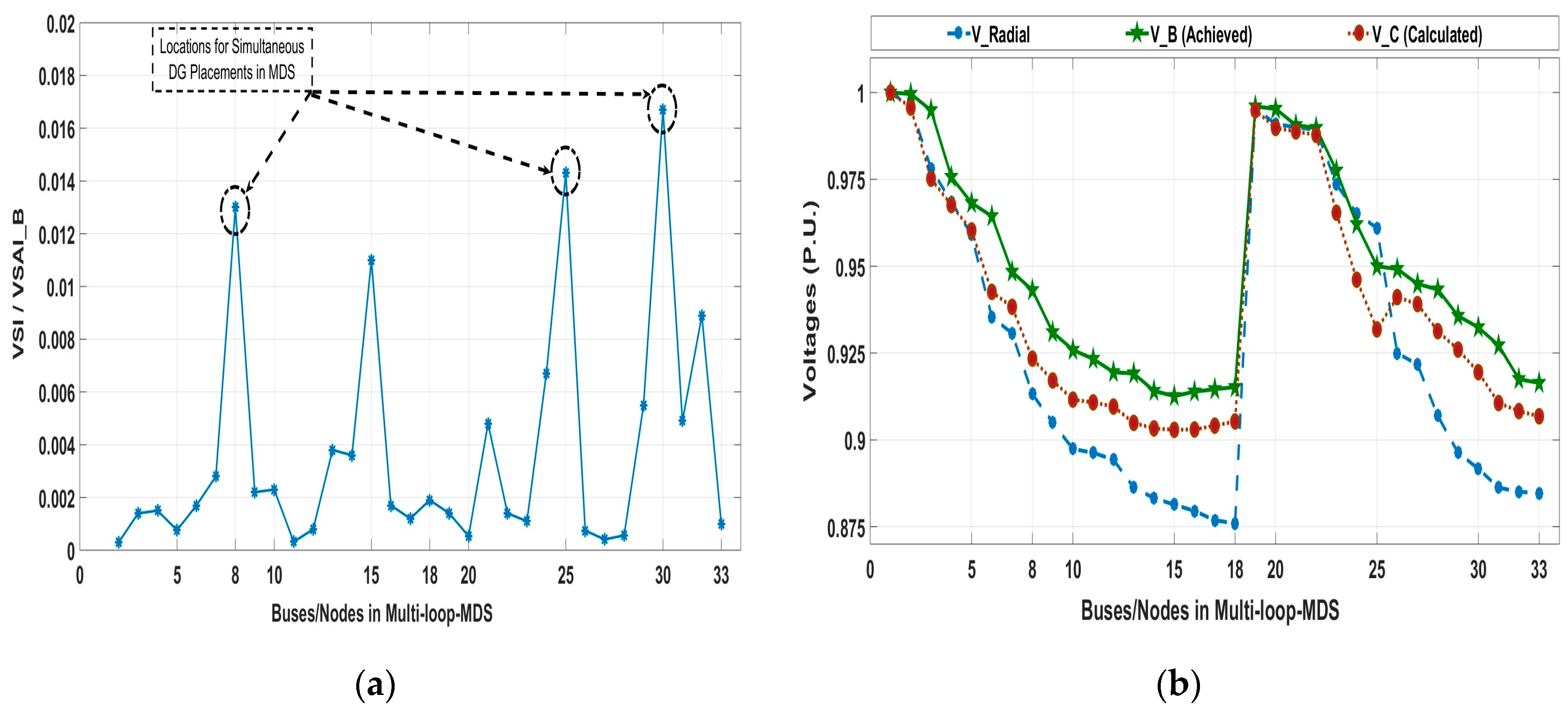
Case 0/Scenario 1 (C0/S1). Base case for potential DG/asset location in 33-bus TDS.

➢

Case 0/Scenario 2 (C0/S2). Base case for potential DG/asset location in 69-bus TDS.

The initial revaluation for 33-bus TDS with VSAI_B in Equation (18) (Steps 1–4 of the computation procedure) for simultaneous multiple DG placements for each case is illustrated in Figure 4a and V_B in Equation (19) as a feasible solution is demonstrated in Figure 4b, respectively.

It is important to mention that VSAI_B evaluation in Figure 4a displays the highest numerical value for 33-bus MDS results in three most optimal locations for simultaneous DG placements. The bus/node 30 of 33-bus TDS is the topmost candidate with numerical value of VSAI_B that is 0.0167 P.U, followed by bus/node 25 with a value of 0.0143 P.U and terminating at bus/node 8 with a value of 0.0130 P.U, respectively. The nodes (buses) with the highest value of VSAI_B value is the potential candidate for DG or asset placement followed by second highest value for second and third highest value of VSAI_B for third DG, respectively. The achieved voltage feasible solution in Figure 4b (of VSAI_B) as V_B is verified by comparing with calculated value V_C (in equivalent Simulink model in Matlab 2017a) to show the feasibility of the obtained solution.

It is interesting to see that both trends (V_B and V_C) closely follows each other, hence establishing an initial verification of the proposed approach at 0 DG case. The weakest node in terms of voltage for the 33-bus MDS in our base case scenario corresponds to V_B and V_C having numerical values of 0.9029 and 0.9128 P.U at node 15, respectively. However, in the radial topology node 65 is the weakest node with the voltage having a numerical value of 0.874 P.U. It is important to mention that readings from radial topology have only mentioned for comparison of variance after a change of topology.

Similarly, the VSAI_B evaluation for 69-bus MDS is illustrated in Figure 5a with the highest numerical values of VSAI_B found as 0.0877 at bus 61, 0.0080 at bus 21 and 0.0038 at bus 11, as most suitable candidates for simultaneous DG placements (considering in hierarchical manner DG1, DG2 and DG3.) in MDS, respectively. The V_B and V_C profiles also correlate closely to demonstrate the initial validation at zero DG level, as demonstrated in Figure 5b for the 69-bus MDS. The weakest node in terms of voltage for 69-bus TDS in the base case scenario exhibits numerical values of V_B and V_C equal to 0.9200 and 0.9221 P.U, respectively. It is observed in both Figure 4b and Figure 5b that the respective voltage profiles of both TDS in the various buses falls under the minimum permissible/allowable voltage limit that is 0.95 (P.U). The initial parameters and findings without DG integration for base cases for both TDS are summarized in

Table 4. Overview of performance in base case without DG as Case 0 (33-bus and 69-bus).

S#:	Technical Parameters (TP)					Cost-Economics Parameters (CP)
C(#)/S(#)	TDS	P & Q Losses (KW + jKVAR)	PL & QL (Load) (KW + jKVAR)	VSAI_B (P.U) @ Bus Location *	Capacity from SS (KW + jKVAR)	PLC (Million USD$)	PLS/AIC (Million USD$)	CPDG ($/MWh)/CQDG ($/MVAR)
C0/S1	33-bus	211 + j 143	3715 + j 2300	0.0167@30 0.0143@25 0.0130@8	3926 + j 2443	0.110902	-	-
C0/S2	69-bus	225.01 + j 102.12	3802.6 + j 2694	0.0877@61 0.0080@21 0.0038@11	4027.61 + j 2796.12	0.118265	-	-

C(#)/S(#) = Case(No.)/Scenario (No.); ^* VSAI_B values have found in MDS.

. The numerical values in Table 4 (except VSAI_B values) show the initial RDS values before meshing and serve as reference parameters for further improvements with proposed approach after considering the mesh topology.

5.2. Detailed Analysis of DG Scenarios at Unity, 0.9 and 0.85 PF on 33-Bus System (Cases 1–3)

The cases 1–3 (C1–C3) correspond to the VSAI-B -LMC based planning approach, which deals with the simultaneous placements of 3 DGs operating at various PF and respective evaluations (steps 5–8 of the computation procedure in Section 4.1). Also, except unity PF, an allowable variation of ±3% in lagging PF is considered. The evaluation for each case has organized in accordance with the various number of scenarios (S#) mainly focusing single to multiple DGs and assets integration, which are further assessed in accordance with computation procedure of proposed approach.

5.2.1. Evaluation of Case 1: DG Placements at unity PF (Type-1)

The proposed approach is initially applied with various number of DGs operating at unity PF (referred to as type-1 in Section 4.4.3) and concerned scenarios have illustrated as follows:

➢

Case 1/Scenario 1 (C1/S1). 1 × DG (at unity PF) placement in the 33-bus MDS.

➢

Case 1/Scenario 2 (C1/S2). 2 × DGs (at unity PF) placement in the 33-bus MDS.

➢

Case 1/Scenario 3 (C1/S3). 3 × DGs (at unity PF) placement in the 33-bus MDS.

The DGs are placed on the basis of Steps 1–4 of the computation and respective sizing is evaluated with LMC between Steps 5–7. The final evaluation is carried out with performance indices of both technical and cost-related nature as aforementioned in Section 4.4, in accordance with step 8 of the computation procedure. The achieved VSAI_B (Equation (18)) trends for case 1 and respective scenarios is illustrated in Figure 6a. The achieved voltage feasible solution of VSAI_B illustrated as V_B (Equation (19)) is shown with V_C for comparison in Figure 6b. All values in Figure 6a,b are in P.U.

It can be observed in Figure 6a that with the integration of one DG at node 30 with a capacity of 3335 KW in C1/S1, the proposed VSAI_B falls to negative value of −0.0513, showing the stability limit. From Figure 6b, V_B has also found to have a correlation with V_C with a numerical value of 1.0 P.U. The minimum voltage in C1/S1 is attained at node/bus 12 with a numerical value of 0.9771 P.U.

The scenario C1/S2 corresponds to simultaneous placements of two DG and VSAI_B limits at node 30 and node 25 concluded in the numerical values of −0.0322 and −0.0172, considering DG capacities (DGC) of 2356 KW and 1351 KW, respectively. The V_B is found to have values of 1.0 P.U at node 30 and 0.9989 P.U at node 25, respectively. The weakest node in C1/S2 is node 13 with V_B around 0.9782 P.U.

The scenario C1/S3 indicates simultaneous placements of three DGs at node 30 (DGC = 1954 KW), node 25 (DGC = 802 KW) and node 8 (DGC = 1001 KW) corresponds to VSAI_B values (in the P.U) such as −0.0245, −0.0005 and −0.0312, respectively. V_B for node 30, 25 and 8 (in P.U) comes out to be around 0.9970, 0.9955 and 0.9947 P.U., respectively. The weakest node in C1/S3 is node 15 with V_B around 0.9839 P.U. The LMC from the perspective of voltage difference ΔU across each tie branch in case 1 in each respective scenario for achieved (V_B values shown in bold letters) and calculated values (V_C) are all presented in (P.U), have shown in relative comparison as follows:

●

C1/S1: ΔU across TB1 (TS4: node 25–29): V_B at 25: 0.9909; V_B at 29: 0.9983; |ΔU_B| = 0.0074.

●

C1/S1: ΔU across TB2 (TS5: node 18–33): V_B at 18: 0.9878; V_B at 33: 0.9877; |ΔU_B| = 0.0001.

●

C1/S1: ΔU across TB1 (TS4: node 25–29): V_C at 25: 0.9927; V_C at 29: 0.9947; |ΔU_C| = 0.0020.

●

C1/S1: ΔU across TB2 (TS5: node 18–33): V_C at 18: 0.9862; V_C at 33: 0.9882; |ΔU_C| = 0.0020.

➢

C1/S2: ΔU across TB1 (TS4: node 25–29): V_B at 25: 1.0000; V_B at 29: 0.9983; |ΔU_B| = 0.0017.

➢

C1/S2: ΔU across TB2 (TS5: node 18–33): V_B at 18: 0.9880; V_B at 33: 0.9887; |ΔU_B| = 0.0007.

➢

C1/S2: ΔU across TB1 (TS4: node 25–29): V_C at 25: 0.9989; V_C at 29: 0.9977; |ΔU_C| = 0.0012.

➢

C1/S2: ΔU across TB2 (TS5: node 18–33): V_C at 18: 0.9865; V_C at 33: 0.9884; |ΔU_C| = 0.0019.

❖

C1/S3: ΔU across TB1 (TS4: node 25–29): V_B at 25: 0.9962; V_B at 29: 0.9954; |ΔU_B| = 0.0008.

❖

C1/S3: ΔU across TB2 (TS5: node 18–33): V_B at 18: 0.9877; V_B at 33: 0.9887; |ΔU_B| = 0.0010.

❖

C1/S3: ΔU across TB1 (TS4: node 25–29): V_C at 25: 0.9955; V_C at 29: 0.9951; |ΔU_C| = 0.0004.

❖

C1/S3: ΔU across TB2 (TS5: node 18–33): V_C at 18: 0.9869; V_C at 33: 0.9880; |ΔU_C| = 0.0011.

It is observed that the LMC is obtained with better numerical values in third scenario (C1/S3) in terms of both V_B and V_C values. The near correlation of voltage difference indicates the suitability of asset capacity and the resulting solution. The V_B values are highlighted for the purpose of differentiation in comparison with V_C values.

The TPI (or TP) evaluation for the case 1 is illustrated in

Table 5. (a) Overview of technical performance evaluation analysis in Case 1 for 33-bus TDS. (b) Overview of Cost-Economics performance evaluation analysis in Case 1 for 33-bus TDS.

S#:	(a) Technical Performance Indicators/Parameters (TPI or TP)
Case(No.)/Scenario (Number)	DG Size (KW) at Bus Location	PLoss (KW)	QLoss (KVAR)	PLM (%)	QLM (%)	DGPP (%)	PSSR (KW)	QSSR (KVAR)
C1/S1 (PF = 1)	DG1: 3335@30	95.88	72.21	54.56	49.503	76.32	475.88	2372.21
C1/S2 (PF = 1)	DG1: 2356@30	88.34	66.44	58.132	53.538	84.84	96.34	2366.44
	DG2: 1351@25
C1/S3 (PF = 1)	DG1: 1954@30	70.78	50.06	66.455	64.993	85.985	28.78	2350.06
	DG2: 802@25
	DG3: 1001@8
S#:	(b) Cost (Economics related) Indicators/Parameters (CPI or CP)
Case(No.)/Scenario (Number)	DG Size (KW) at Bus Location	PLC (Million USD$)	PLS (Million USD$)	CPDG ($/MWh)	CQDG ($/MVAr-h)	AIC (1) (Million USD$)	AIC (2) (Million USD$)		(ACD) (Million USD$)
C1/S1 (PF = 1)	3335@30	0.050395	0.06051	66.95	0	0.8819	0.6299		0
C1/S2 (PF = 1)	2356@30	0.046432	0.06447	74.39	0	0.9803	0.7003		0
	1351@25
C1/S3 (PF = 1)	1954@30	0.03720	0.0737	75.35	0	0.9936	0.7097		0
	802@25
	1001@8

a (considering the base case as reference). The achieved results in Table 5a have been evaluated against the achieved power losses with percentage minimizations, achieved DGPP and active/reactive power relief to substation within various scenarios. In comparison, the best scenario within case 1 comes out to be C1/S3. The active and reactive power losses achieved have values of 70.78 KW and 50.06 KVAR, respectively. The active and reactive loss minimizations have attained values of 66.455% and 6.4993% respectively. It is also important to mention that the high contribution of active power from DG also contributes to reduction in reactive power losses. Besides, achieved DGPP is 85.985%, the contribution of substation in active power component is 28.78 KW, which although is within limit, however, a further increase in active component from DG may result in reverse power flow.

The CPI (or CP) evaluation of proposed approach for the offered case 1 is illustrated in Table 5b (considering the base case as reference). The evaluations in Table 5b have evaluated against cost of active power losses (PLC), savings due to active power reduction (PLS), cost of active (CPDG) and reactive power (CQDG) from the DG units and annual investment cost (AIC), respectively. The scenario C1/S3 out performs all others in-terms of minimum PLC (0.03720 million USD or M$) and highest PLS (0.0737 M$). However, more active component contribution form DG results in more numerical value of 75.35 $/MWh (in C1/S3) in comparison with other scenarios such as 74.39 $/MWh in C1/S2 and 66.95 $/MWh in C1/S2, respectively. In terms of AIC, two evaluations have considered [29,35]. In our previous publication, the cost (CUc) of type-1 DG unit was considered 5250 $/KW in year 2011–2012 [26,29,35]. However, the prices of solar are expected down to around 3750 $/KWh in year 2019–2020 and can compete other technologies on the basis of cost of economics [49]. Hence, AIC values for each scenario is calculated for both values for evaluation and verification. On the basis of old reading of CUc (5250 $/KW), AIC comes out to be 0.9936 M$. Whereas with modified values of CUc (3750 $/KWh), evaluated AIC value is 0.7097 M$.

5.2.2. Evaluation of Case 2: DG Placements at 0.90 ± 3% PF lagging (Type-2)

The proposed approach is applied with single and multiple number DGs operating at 0.90 ± 3% lagging PF, which is favored by the electrical utilities. DG, in this case, referred to as type-2 (in Section 4.4.3) and concerned scenarios are illustrated as follows:

➢

Case 2/Scenario 1 (C2/S1): 1 × DG (at 0.90 ± 3% lagging PF) placement in the 33-bus MDS.

➢

Case 2/Scenario 2 (C2/S2): 2 × DGs (at 0.90 ± 3% lagging PF) placement in the 33-bus MDS.

➢

Case 2/Scenario 3 (C2/S3): 3 × DGs (at 0.90 ± 3% lagging PF) placement in the 33-bus MDS.

In case 2, single and multiple DGs are placed in the same manner as illustrated in the previous case 1. The only difference is the DGs operating at 0.90 ± 3% lagging PF. The VSAI_B trend (via Equation (18)) and associated voltage profile V_B (via Equation (19)) for case 2 is illustrated in Figure 7a,b, respectively. The important observations of VSAI_B in Figure 7a and V_B in Figure 7b, are indicated as follows:

❖

VSAI_B and V_B values of DG in C2/S1 in (P.U):

○ VSAI_B for DG1@bus 30:	−0.0565@30
○ V_B for DG1@bus 30:	1.0000@30
○ Minimum voltage (V_min):	0.9764@12

❖

VSAI_B and V_B values of DG in C2/S2 in (P.U):

○ VSAI_B for DG1@30 and DG2@25:	−0.0462@30; −0.0021@25
○ V_B for DG1@30 and DG2@25:	0.9999@30; 0.9958@25
○ Minimum voltage (V_min):	0.9769@13

❖

VSAI_B and V_B values of DG in C2/S3 in (P.U):

○ VSAI_B for DG1@30; DG2@25; DG3@8:	−0.0358@30; −0.0010@25; −0.0281@8
○ V_B for DG1@30; DG2@25; DG3@8:	1.0000@30; 0.9966@25; 0.9956@8
○ Minimum voltage (V_min):	0.9857@15

The LMC in terms of voltage difference (ΔU) across each TB in case 2 in each respective scenario for achieved (V_B) and calculated values (V_C) in P.U, are shown as follows (the V_B values are highlighted in bold font for the purpose of differentiation in comparison with V_C values):

●

C2/S1: ΔU across TB1 (TS4: node 25–29): V_B at 25: 0.9928; V_B at 29: 0.9954; |ΔU_B| = 0.0026.

●

C2/S1: ΔU across TB2 (TS5: node 18–33): V_B at 18: 0.9859; V_B at 33: 0.9880; |ΔU_B| = 0.0021.

●

C2/S1: ΔU across TB1 (TS4: node 25–29): V_C at 25: 0.9925; V_C at 29: 0.9965; |ΔU_C| = 0.0040.

●

C2/S1: ΔU across TB2 (TS5: node 18–33): V_C at 18: 0.9877; V_C at 33: 0.9894; |ΔU_C| = 0.0017.

➢

C2/S2: ΔU across TB1 (TS4: node 25–29): V_B at 25: 0.9958; V_B at 29: 0.9966; |ΔU_B| = 0.0008.

➢

C2/S2: ΔU across TB2 (TS5: node 18–33): V_B at 18: 0.9860; V_B at 33: 0.9880; |ΔU_B| = 0.0020.

➢

C2/S2: ΔU across TB1 (TS4: node 25–29): V_C at 25: 0.9966; V_C at 29: 0.9983; |ΔU_C| = 0.0017.

➢

C2/S2: ΔU across TB2 (TS5: node 18–33): V_C at 18: 0.9876; V_C at 33: 0.9894; |ΔU_C| = 0.0018.

❖

C2/S3: ΔU across TB1 (TS4: node 25–29): V_B at 25: 0.9966; V_B at 29: 0.9975; |ΔU_B| = 0.0009.

❖

C2/S3: ΔU across TB2 (TS5: node 18–33): V_B at 18: 0.9894; V_B at 33: 0.9907; |ΔU_B| = 0.0013.

❖

C2/S3: ΔU across TB1 (TS4: node 25–29): V_C at 25: 0.9960; V_C at 29: 0.9983; |ΔU_C| = 0.0023.

❖

C2/S3: ΔU across TB2 (TS5: node 18–33): V_C at 18: 0.9903; V_C at 33: 0.9904; |ΔU_C| = 0.0001.

The TP evaluation for case 2 is shown in self-explanatory manner as illustrated in

Table 6. (a) Overview of technical performance evaluation analysis in case 2 for 33-bus TDS. 6 (b). Overview of Cost-Economics performance evaluation analysis in case 2 for 33-bus TDS.

S#:	(a) Technical Parameters (TP)
Case(No.)/Scenario (Number)	DG Size (KVA)@ Bus Location	PLoss (KW)	QLoss (KVAR)	PLM (%)	QLM (%)	DGPP (%)	PSSR (KW)	QSSR (KVAR)
C2/S1 (PF = 0.90 ± 3%)	DG1: 2750@30	38.3	28.933	81.85	79.76	62.937	1278.3	1130.233
C2/S2 (PF = 0.90 ± 3%)	DG1: 2357@30	32.99	25.491	84.37	82.17	66.303	1140.69	1062.718
	DG2: 540@25
C2/S3 (PF = 0.90 ± 3%)	DG1: 1957@30	18.87	13.327	91.06	90.68	73.625	838.57	911.069
	DG2: 500@25
	DG3: 760@8
S#:	(b) Cost (Economics related) Parameters (CP)
Case(No.)/Scenario (Number)	DG Size (KVA) @ Bus Location	PLC (Million USD$)	PLS (Million USD$)	CPDG ($/MWh)	CQDG ($/MVArh)	AIC (1) (Million USD$)	AIC (2) (Million USD$)	(ACD) (Million USD$)
C2/S1 (PF = 0.90 ± 3%)	2750@30	0.02013	0.09077	49.75	4.9527	0.4969	0.4969	0
C2/S2 (PF = 0.90 ± 3%)	2357@30	0.01261	0.09829	52.396	5.2141	0.5235	0.5235	0
	540@25
C2/S3 (PF = 0.90 ± 3%)	1957@30	0.00992	0.1010	58.156	5.7938	0.5813	0.5813	0
	500@25
	760@8

DG size is shown in KVA @ PF = 0.9 ± 3%; Site is shown by at or symbol @ bus No. in TDS.

a (considering the base case as reference), which indicates a substantial power loss minimization is achieved along with considerable DG penetration. The main difference between case 1 and case 2 is the type of the DG. The type-2 DG is contributing both active and reactive power support near the allocated respective load buses and a considerable reduction in losses have observed in case 2 as compared to case 1. The DG capacity is also reduced and provides more losses minimization at comparatively less penetration. The relief on the substation is also reduced in comparison with the base case scenario and it is not liable to reverse power flow in case on any other active and reactive power component contribution from DG units. The relative comparative analysis of TP based results between case 1 and case 2 are illustrated as follows:

❖

Percentage improvement in TP between case 2 (DGs with PF ± 3%) and case 1 (DGs with 1 PF).

○

Reduction (↓) in P_Loss by% in case 2 (S1, S2 & S3): 60.10% (↓); 62.66% (↓); 73.34% (↓).

○

Reduction (↓) in Q_Loss by% in case 2 (S1, S2 & S3): 59.85% (↓); 61.63% (↓); 73.40% (↓).

○

Increase (↑) in DGPP by% in case 2 (S1, S2 & S3): −17.54% (↑); −21.85% (↑); −14.37% (↑).

The CP evaluation of case 2 is illustrated in Table 6b (considering the base case as reference). A substantial improvement in all CPIs has observed in case 2 along with evaluations of the respective scenarios. In addition to Table 6b, the relative comparative analysis of case 2 with case 1 (as relative reference), suggests significant improvements in achieved performance indicators. The relative comparative analysis in terms of CP based results achieved in case 2 in comparison with case 1, indicates the following observations along with the achieved results and are illustrated as follows:

❖

Percentage improvement in CP of case 2 (DGs with PF ± 3%) in contrast to case 1 (DGs with 1 PF).

○

Reduction (↓) in PLC by% in case 2 (S1, S2 & S3): 60.05% (↓); 72.84% (↓); 73.33% (↓).

○

Increase (↑) in PLS by% in case 2 (S1, S2 & S3): 50.01% (↑); 52.46% (↑); 37.04% (↑).

○

Reduction (↓) in CPDG by% in case 2 (S1, S2 & S3): 25.69% (↓); 29.57% (↓); 22.82% (↓).

○

Reduction (↓) in AIC (1) by% in case 2 (S1, S2 & S3): 43.66% (↓); 46.60% (↓); 41.50% (↓).

○

Reduction (↓) in AIC (2) by% in case 2 (S1, S2 & S3): 21.11% (↓); 25.25% (↓); 18.10% (↓).

5.2.3. Evaluation under Case 3: DG Placements at 0.85 ± 3% PF (Type-2)

The proposed approach is applied with single and multiple number DGs operating at 0.85 ± 3% lagging PF considering load PF of TDS. The DG is type-2 operating at 0.85 ± 3% lagging PF (in Section 4.4.3) and concerned scenarios have illustrated as follows:

➢

Case 3/Scenario 1 (C3/S1): 1 × DG (at 0.85 ± 3% lagging PF) placement in the 33-bus MDS.

➢

Case 3/Scenario 2 (C3/S2): 2 × DGs (at 0.85 ± 3% lagging PF) placement in the 33-bus MDS.

➢

Case 3/Scenario 3 (C3/S3): 3 × DGs (at 0.85 ± 3% lagging PF) placement in the 33-bus MDS.

In case 3, single and multiple DGs are operating at 0.85 ± 3% lagging PF and placed with the same computational procedure as previously employed in cases 1 and 2. The VSAI_B trend (via Equation (18)) and associated voltage profile V_B (via Equation (19)) for case 3 is illustrated in Figure 8a,b, respectively. The observations of VSAI_B and V_B for case 3 is illustrated as follows:

❖

VSAI_B and V_B values of DG in C3/S1 in (P.U):

○ VSAI_B for DG1@bus 30:	−0.0570@30
○ V_B for DG1@bus 30:	0.9998@30
○ Minimum voltage (V_min):	0.9761@12

❖

VSAI_B and V_B values of DG in C3/S2 in (P.U):

○ VSAI_B for DG1@ 30 and DG2@25:	−0.0351@30; −0.0203@25
○ V_B for DG1@ 30 and DG2@25:	1.0000@30; 0.9995@25
○ Minimum voltage (V_min):	0.9773@13

❖

VSAI_B and V_B values of DG in C3/S3 in (P.U):

○ VSAI_B for DG1@30; DG2@25; DG3@8:	−0.0228@30; −0.0168@25; −0.0377@8
○ V_B for DG1@30; DG2@25; DG3@8:	1.0000@30; 1.0000@25; 0.9998@8
○ Minimum voltage (V_min):	0.9880@15

The comparative voltage difference across tie-line branches is indicated in terms of V_B and V_C values in (P.U). The V_B values are highlighted for the purpose of differentiation in contrast to V_C values.

●

C3/S1: ΔU across TB1 (TS4: node 25–29): V_B at 25: 0.9927; V_B at 29: 0.9953; |ΔU_B| = 0.0026.

●

C3/S1: ΔU across TB2 (TS5: node 18–33): V_B at 18: 0.9856; V_B at 33: 0.9877; |ΔU_B| = 0.0021.

●

C3/S1: ΔU across TB1 (TS4: node 25–29): V_C at 25: 0.9954; V_C at 29: 0.9982; |ΔU_C| = 0.0028.

●

C3/S1: ΔU across TB2 (TS5: node 18–33): V_C at 18: 0.9878; V_C at 33: 0.9892; |ΔU_C| = 0.0014.

➢

C3/S2: ΔU across TB1 (TS4: node 25–29): V_B at 25: 0.9995; V_B at 29: 0.9984; |ΔU_B| = 0.0011.

➢

C3/S2: ΔU across TB2 (TS5: node 18–33): V_B at 18: 0.9862; V_B at 33: 0.9882; |ΔU_B| = 0.0020.

➢

C3/S2: ΔU across TB1 (TS4: node 25–29): V_C at 25: 0.9982; V_C at 29: 0.9983; |ΔU_C| = 0.0001.

➢

C3/S2: ΔU across TB2 (TS5: node 18–33): V_C at 18: 0.9878; V_C at 33: 0.9896; |ΔU_C| = 0.0018.

❖

C3/S3: ΔU across TB1 (TS4: node 25–29): V_B at 25: 1.0000; V_B at 29: 0.9992; |ΔU_B| = 0.0008.

❖

C3/S3: ΔU across TB2 (TS5: node 18–33): V_B at 18: 0.9904; V_B at 33: 0.9914; |ΔU_B| = 0.0010.

❖

C3/S3: ΔU across TB1 (TS4: node 25–29): V_C at 25: 0.9990; V_C at 29: 0.9976; |ΔU_C| = 0.0014.

❖

C3/S3: ΔU across TB2 (TS5: node 18–33): V_C at 18: 0.9910; V_C at 33: 0.9908; |ΔU_C| = 0.0002.

The TP evaluation for case 3 in comparison with the base case is illustrated in

Table 7. (a) Overview of technical performance evaluation analysis in case 3 (33-bus). (b) Overview of Cost-economics performance evaluation analysis in case 3 (33-bus).

S#:	(a) Technical Parameters (TP)
Case(No.)/Scenario (Number)	DG Size (KW)/Bus Location	PLoss (KW)	QLoss (KVAR)	PLM (%)	QLM (%)	DGPP (%)	PSSR (KW)	QSSR (KVAR)
C3/S1 (PF = 0.85 ± 3%)	DG1:2708.8@30	35.20	28.98	83.32	79.73	61.993	1447.720	902.030
C3/S2 (PF = 0.85 ± 3%)	DG1:1885.8@30	27.93	24.39	86.76	82.94	69.874	1147.712	716.587
	DG2:1167.4@25
C3/S3 (PF = 0.85 ± 3%)	DG1:1422.1@30	13.85	11.50	93.44	91.96	77.834	838.085	519.965
	DG2:1045.4@25
	DG3:933.4@8
S#:	(b) Cost (Economics related) Parameters (CP)
Case(No.)/Scenario (Number)	DG Size (KW)/Bus Location	PLC (Million USD$)	PLS (Million USD$)	CPDG ($/MWh)	CQDG ($/MVArh)	AIC (1) (Million USD$)	AIC (2) (Million USD$)	(ACD) (Million USD$)
C3/S1 (PF = 0.85 ± 3%)	2708.8@30	0.01850	0.09240	46.298	7.2777	0.4895	0.4895	0
C3/S2 (PF = 0.85 ± 3%)	1885.8@30	0.01468	0.09622	52.1529	8.2030	0.5517	0.5517	0
	1167.4@25
C3/S3 (PF = 0.85 ± 3%)	1422.1@30	0.00728	0.10362	58.0651	9.1375	0.6145	0.6145	0
	1045.4@25
	933.4@8

a, with the deployment of type-2 DGs operating at 0.85 ± 3% lagging PF and contributing more reactive power support as compared to that in case 2. Improvements can be observed in various TPIs such as P_Loss, Q_Loss and DGPP. The relative comparative analysis of TP based results among case 3 and case 1 are illustrated as follows. It is important to mention that case 2 is shown for relative reference and result values for case 3 has shown in bold. The relative comparative analysis of case 2 and case 3 indicates a further reduction in P_Loss, Q_Loss and DGPP in comparison with case 1.

○

Reduction (↓) in P_Loss by% in case 2 (S1, S2 & S3): 60.10% (↓); 62.66% (↓); 73.34% (↓).

➢

Reduction (↓) in P_Loss by% in case 3 (S1, S2 & S3): 63.29% (↓); 68.38% (↓); 80.43% (↓).

○

Reduction (↓) in Q_Loss by% in case 2 (S1, S2 & S3): 59.85% (↓); 61.63% (↓); 73.40% (↓).

➢

Reduction (↓) in Q_Loss by% in case 3 (S1, S2 & S3): 59.86% (↓); 63.29% (↓); 70.03% (↓).

○

Increase (↑) in DGPP by% in case 2 (S1, S2 & S3): −17.54% (↑); −21.85% (↑); −14.37% (↑).

➢

Increase (↑) in DGPP by% in case 3 (S1, S2 & S3): −18.77% (↑); −17.64% (↑); −9.48% (↑).

The CP evaluation of case 3 is illustrated in Table 7b (considering the base case as reference). The relative comparative analysis in terms of CP based results between case 2, case 3 with reference to case 1 are illustrated as follows (note: The case 2 is shown for reference and case 3 is shown in bold):

❖

Percentage improvement in CP between case 2, 3 and case 1:

○

Reduction (↓) in PLC by% in case 2 (S1, S2 & S3): 60.05% (↓); 72.84% (↓); 73.33% (↓).

➢

Reduction (↓) in PLC by% in case 3 (S1, S2 & S3): 63.29% (↓); 68.38% (↓); 80.43% (↓).

○

Increase (↑) in PLS by% in case 2 (S1, S2 & S3): 50.01% (↑); 52.46% (↑); 37.04% (↑).

➢

Increase (↑) in PLS by% in case 3 (S1, S2 & S3): 52.70% (↑); 49.25% (↑); 40.60% (↑).

○

Reduction (↓) in CPDG by% in case 2 (S1, S2 & S3): 25.69% (↓); 29.57% (↓); 22.82% (↓).

➢

Reduction (↓) in CPDG by% in case 3 (S1, S2 & S3): 30.85% (↓); 29.89% (↓); 22.94% (↓).

○

Reduction (↓) in AIC (1) by% in case 2 (S1, S2 & S3): 43.66% (↓); 46.60% (↓); 41.50% (↓).

➢

Reduction (↓) in AIC (1) by% in case3 (S1, S2 & S3): 44.50% (↓); 43.72% (↓); 38.15% (↓).

○

Reduction (↓) in AIC (2) by% in case 2 (S1, S2 & S3): 21.11% (↓); 25.25% (↓); 18.10% (↓).

➢

Reduction (↓) in AIC (2) by% in case3 (S1, S2 & S3): 22.29% (↓); 21.21% (↓); 13.41% (↓).

The relative comparative analysis of case 2 and case 3 indicates a further reduction in PLC in comparison with case 1 for scenario C3/S3 only. The PLS is comparatively higher in C3/S1 and C3/S3. However, CPDG is greater in case 3 than the results achieved in case 2. However, on the basis of AIC, case 3 is comparatively less cost-effective as compared to case 2, except for C3/S1.

5.3. Detailed Analysis of Assets (DG+DSTATCOM) Placements Scenarios in 33-bus System (Cases 4–5)

5.3.1. Evaluation under Case 4: DG (Type-1) and DSTATCOM (Type-3) Placements

The proposed approach is applied with single and multiple number of DGs and D-STATCOM (DSt) placement. The DG and DSt in case 4 is separately contributing active and reactive power equivalent to case 2 (provided by type-2 DGs only and operating at 0.90 ± 3% lagging PF).

➢

Case 4/Scenario 1 (C4/S1): 1 × DG + 1 × DSTATCOM placement in the 33-bus MDS.

➢

Case 4/Scenario 2 (C4/S2): 2 × DG + 2 × DSt placement in the 33-bus MDS.

➢

Case 4/Scenario 3 (C4/S3): 3 × DG + 3 × DSt placement in the 33-bus MDS.

In case 4, a set of type-1 DGs and type-3 DSts, is placed on the same bus/node such that their active and reactive power contribution matches that of DGs operating at 0.90 ± 3% lagging PF. Although the authors have justified the same and separate locations for DG type-1 and DSt installation on a bus/node, however, in this study, a set of each DG is placed along with a DSt and the resulting performance is evaluated. The VSAI_B trend (via Equation (18)) and associated voltage profile (via Equation (19)) for case 4 is illustrated in Figure 9a,b, respectively.

The observations of VSAI_B and V_B for case 4 is illustrated as follows (note: all values are in P.U):

❖

VSAI_B and V_B values of DG + DSTATCOM (DG + DSt) in C4/S1:

○ VSAI_B for DG1 + DSt1@bus 30:	−0.0560@30
○ V_B for DG1 + DSt1@bus 30:	0.9999@30
○ Minimum voltage (V_min):	0.9764@12

❖

VSAI_B and V_B values of DG + DSt in C4/S2:

○ VSAI_B for DG1 + DSt1@30 and DG2 + DS2@25:	−0.0459@30; −0.0210@25
○ V_B for DG1 + DSt1@30 and DG2 + DS2@25:	0.9998@30; 0.9957@25
○ Minimum voltage (V_min):	0.9768@13

❖

VSAI_B and V_B values of DG + DSt in C3/S3:

○ VSAI_B for DG1 + DSt1@30; DG2 + DSt2@25; DG3 + DSt3@8:	−0.0356@30; −0.001@25; −0.0280@8
○ V_B for DG1 + DSt1@30; DG2 + DSt2@ 25; DG3 + DSt3@8:	1.0000@30; 0.9966@25; 0.9955@8
○ Minimum voltage (V_min):	0.9856@15

The comparative voltage difference (ΔU) across TBs (TB1 and TB2) for case 4, is indicated in terms of V_B (highlighted in bold font) and V_C values in P.U, respectively.

●

C4/S1: ΔU across TB1 (TS4: node 25–29): V_B at 25: 0.9928; V_B at 29: 0.9953; |ΔU_B| = 0.0025.

●

C4/S1: ΔU across TB2 (TS5: node 18–33): V_B at 18: 0.9858; V_B at 33: 0.9879; |ΔU_B| = 0.0021.

●

C4/S1: ΔU across TB1 (TS4: node 25–29): V_C at 25: 0.9906; V_C at 29: 0.9983; |ΔU_C| = 0.0077.

●

C4/S1: ΔU across TB2 (TS5: node 18–33): V_C at 18: 0.9875; V_C at 33: 0.9894; |ΔU_C| = 0.0019.

➢

C4/S2: ΔU across TB1 (TS4: node 25–29): V_B at 25: 0.9957; V_B at 29: 0.9965; |ΔU_B| = 0.0001.

➢

C4/S2: ΔU across TB2 (TS5: node 18–33): V_B at 18: 0.9858; V_B at 33: 0.9879; |ΔU_B| = 0.0021.

➢

C4/S2: ΔU across TB1 (TS4: node 25–29): V_C at 25: 0.9960; V_C at 29: 0.9982; |ΔU_C| = 0.0022.

➢

C4/S2: ΔU across TB2 (TS5: node 18–33): V_C at 18: 0.9875; V_C at 33: 0.9893; |ΔU_C| = 0.0018.

❖

C4/S3: ΔU across TB1 (TS4: node 25–29): V_B at 25: 0.9966; V_B at 29: 0.9975; |ΔU_B| = 0.0011.

❖

C4/S3: ΔU across TB2 (TS5: node 18–33): V_B at 18: 0.9893; V_B at 33: 0.9907; |ΔU_B| = 0.0014.

❖

C4/S3: ΔU across TB1 (TS4: node 25–29): V_C at 25: 0.9970; V_C at 29: 0.9982; |ΔU_C| = 0.0012.

❖

C4/S3: ΔU across TB2 (TS5: node 18–33): V_C at 18: 0.9896; V_C at 33: 0.9914; |ΔU_C| = 0.0008.

The TP evaluation for case 4 is shown in self-explanatory manner as illustrated in

Table 8. (a) Overview of technical performance evaluation analysis in case 4 (33-bus). (b) Overview of Cost-Economics performance evaluation analysis in case 4 (33-bus).

S#:	(a) Technical Parameters (TP)
Case(No.)/Scenario (Number)	DG Size	PLoss	QLoss	PLM	QLM	DGPP	PSSR	QSSR
	KW/KVAr @ Bus Location	(KW)	(KVAR)	(%)	(%)	(%)	(KW)	(KVAR)
C4/S1 (CPF = 0.90 ± 3%)	DG1:2475@30	39	29.382	81.52	79.45	62.94	1279	1130.382
	DSt1:1199@30
C4/S2 (CPF = 0.90 ± 3%)	DG1:2121@30	34	26.807	83.89	81.25	66.305	1142	1062.81
	DSt1:1028@30
	DG2:486@25
	DSt2:236@25
C4/S3 (CPF = 0.90 ± 3%)	DG1:1761@30	20.8	13.761	90.14	90.38	73.63	840.8	911.461
	DSt1:853@30
	DG2:450@25
	DSt2:218@25
	DG3:684@8
	DSt3:331.3@8
S#:	(b) Cost (Economics related) Parameters (CP)
Case(No.)/Scenario (Number)	DG/DSt Size KW/KVAr	PLC	PLS	CPDG ($/MWh)	CQDG ($/MVArh)	AIC (1)	AIC (2)	(ACD)
	@ Bus Location	(Million USD$)	(Million USD$)			(Million USD$)	(Million USD$)	(Million USD$)
C4/S1 (CPF = 0.85 ± 3%)	2475 + j1199 @ 30	0.0205	0.0904	49.749	4.9553	0.6545	0.4675	0.01581
C4/S2 (CPF = 0.85 ± 3%)	2121 + j1028 @ 30	0.0179	0.09303	52.39	5.227	0.6894	0.4925	0.01666
	486 + j236 @ 25
C4/S3 (CPF = 0.85 ± 3%)	1761 + j853 @ 30	0.01093	0.09997	58.1557	5.7941	0.7656	0.5467	0.01849
	450 + j218 @25
	684 + j331.3 @8

a (considering the base case as reference). It has observed that the achieved results as TPIs have found in close approximation in comparison with the numerical results achieved in case 2. The results in case 4 justify the deployment of DSts to increase the optimal penetration of renewable DGs (for example PV-based DGs) usually operating at unity PF. The relative comparative analysis of TP-based results between case 4 and case 2, with reference to the case 1 are illustrated as follows (it is important to mention that case 2 is shown for reference and considered case 4 is shown in bold font):

❖

Percentage improvement in TP between case 2 and case 4 in comparison with case 1:

○

Reduction (↓) in P_Loss by% in case 2 (S1, S2 & S3): 60.10% (↓); 62.66% (↓); 73.34% (↓).

➢

Reduction (↓) inP_Loss by% in case 4 (S1, S2 & S3): 59.32% (↓); 61.51% (↓); 70.61% (↓).

○

Reduction (↓) in Q_Loss by% in case 2 (S1, S2 & S3): 59.85% (↓); 61.63% (↓); 73.40% (↓).

➢

Reduction (↓) inQ_Loss by% in case 4 (S1, S2 & S3): 59.31% (↓); 59.65% (↓); 72.51% (↓).

○

Increase (↑) in DGPP by% in case 2 (S1, S2 & S3): −17.54% (↑); −21.85% (↑); −14.37% (↑).

➢

Increase (↑) inDGPP by% in case 4 (S1, S2 & S3):−17.53% (↑); −25.81% (↑); −14.38% (↑).

The CP evaluation of case 4 is illustrated in Table 8b (considering the base case as reference). Likewise, TP evaluation in Table 8a, the CP results in Table 8b indicates to have found in close approximation with case 2 (previously analyzed). The relative comparative analysis in terms of CP- based results between case 2, case 4 with reference to case 1 are illustrated as follows (note: The case 2 is shown for reference and case 4 is shown in bold font):

❖

Percentage improvement in CP between case 2 (for reference) and case 4 with respect to case 1:

○

Reduction (↓) in PLC by% in case 2 (S1, S2 & S3): 60.05% (↓); 72.84% (↓); 73.33% (↓).

➢

Reduction (↓) in PLC by% in case 4 (S1, S2 & S3): 59.32% (↓); 61.45% (↓); 70.62% (↓).

○

Increase (↑) in PLS by% in case 2 (S1, S2 & S3): 50.01% (↑); 52.46% (↑); 37.04% (↑).

➢

Increase (↑) in PLS by% in case 4 (S1, S2 & S3): 49.40% (↑); 44.30% (↑); 35.65% (↑).

○

Reduction (↓) in CPDG by% in case 2 (S1, S2 & S3): 25.69% (↓); 29.57% (↓); 22.82% (↓).

➢

Reduction (↓) in CPDG by% in case 4 (S1, S2 & S3): 25.69% (↓); 29.57% (↓); 22.82% (↓).

○

Reduction (↓) in AIC (1) by% in case 2 (S1, S2 & S3): 43.66% (↓); 46.60% (↓); 41.50% (↓).

➢

Reduction (↓) in AIC (1) by% in case4 (S1, S2 & S3):25.785% (↓); 29.68% (↓); 22.76% (↓).

○

Reduction (↓) in AIC (2) by% in case 2 (S1, S2 & S3): 21.11% (↓); 25.25% (↓); 18.10% (↓).

➢

Reduction (↓) in AIC (2) by% in case4 (S1, S2 & S3): 22.78% (↓); 29.67% (↓); 22.97% (↓).

5.3.2. Evaluation under Case 5: DG (Type-1) and DSTATCOM (Type-3) Placements

The proposed approach is applied with single and multiple number of DGs and D-STATCOM (DSt) placements. The DG and DSt in case 5 is separately contributing active and reactive power equivalent to case 3 (provided by type-2 DGs only and operating at 0.85 ± 3% lagging PF):

➢

Case 5/Scenario 1 (C5/S1): 1 × DG + 1 × DSTATCOM placement in 33-bus MDS.

➢

Case 5/Scenario 2 (C5/S2): 2 × DG + 2 × DSTATCOM placement in 33-bus MDS.

➢

Case 5/Scenario 3 (C5/S3): 3 × DG + 3 × DSTATCOM placement in 33-bus MDS.

In case 5, type-1 DGs and type-3 DSTATCOMs are placed on the same bus/node such that their active and reactive power contribution matches that of DGs operating at 0.85 ± 3% lagging PF. The DG and DSt set is placed in TDS in the same manner as employed in case 4. The VSAI_B trend (via Equation (18)) and associated voltage profile V_B (via Equation (19)) for case 4 is illustrated in Figure 10a,b, respectively. The observations of VSAI_B and V_B for case 5 is illustrated as follows (note: all values are in P.U):

❖

VSAI_B and V_B values of DG + DSTATCOM (DG + DS) in C5/S1:

○ VSAI_B for DG1 + DSt1 @ bus 30:	−0.0565@30
○ V_B for DG1 + DSt1 @ bus 30:	0.9997@30
○ Minimum voltage (V_min):	0.9760@12

❖

VSAI_B and V_B values of DG + DSt in C5/S2:

○ VSAI_B for DG1 + DSt1@30 and DG2 + DSt2 @25:	−0.0563@30; −0.0202@25
○ V_B for DG1 + DSt1 @30 and DG2 + DSt2 @25:	0.9999@30; 0.9994@25
○ Minimum voltage (V_min):	0.9768@13

❖

VSAI_B and V_B values of DG + DS in C5/S3:

○ VSAI_B for DG1 + DSt1@30; DG2 + DSt2@25; DG3 + DSt3@8:	−0.0228@30; −0.0167@25; −0.0375@8
○ V_B for DG1 + DSt1@30; DG2 + DSt2@25; DG3 + DSt3@ 8:	0.9998@30; 0.9998@25; 0.9997@8
○ Minimum voltage (V_min):	0.9878@15

The comparative voltage difference across tie-line branches for case 5 is indicated in terms of V_B (highlighted) and V_C values in (P.U).

●

C5/S1: ΔU across TB1 (TS4: node 25–29): V_B at 25: 0.9926; V_B at 29: 0.9950; |ΔU_B| = 0.0024.

●

C5/S1: ΔU across TB2 (TS5: node 18–33): V_B at 18: 0.9855; V_B at 33: 0.9876; |ΔU_B| = 0.0021.

●

C5/S1: ΔU across TB1 (TS4: node 25–29): V_C at 25: 0.9942; V_C at 29: 0.9936; |ΔU_C| = 0.0006.

●

C5/S1: ΔU across TB2 (TS5: node 18–33): V_C at 18: 0.9872; V_C at 33: 0.9900; |ΔU_C| = 0.0028.

➢

C5/S2: ΔU across TB1 (TS4: node 25–29): V_B at 25: 0.9994; V_B at 29: 0.9983; |ΔU_B| = 0.0011.

➢

C5/S2: ΔU across TB2 (TS5: node 18–33): V_B at 18: 0.9861; V_B at 33: 0.9881; |ΔU_B| = 0.0020.

➢

C5/S2: ΔU across TB1 (TS4: node 25–29): V_C at 25: 1.0000; V_C at 29: 0.9967; |ΔU_C| = 0.0033.

➢

C5/S2: ΔU across TB2 (TS5: node 18–33): V_C at 18: 0.9877; V_C at 33: 0.9895; |ΔU_C| = 0.0018.

❖

C5/S3: ΔU across TB1 (TS4: node 25–29): V_B at 25: 0.9998; V_B at 29: 0.9990; |ΔU_B| = 0.0008.

❖

C5/S3: ΔU across TB2 (TS5: node 18–33): V_B at 18: 0.9901; V_B at 33: 0.9912; |ΔU_B| = 0.0011.

❖

C5/S3: ΔU across TB1 (TS4: node 25–29): V_C at 25: 1.0000; V_C at 29: 0.9982; |ΔU_C| = 0.0018.

❖

C5/S3: ΔU across TB2 (TS5: node 18–33): V_C at 18: 0.9908; V_C at 33: 0.9918; |ΔU_C| = 0.0010.

The TP evaluation for case 3 in comparison with the base case is illustrated in

Table 9. (a) Overview of technical performance evaluation analysis in case 5 (33-bus). (b) Overview of Cost-Economics performance evaluation analysis in case 5 (33-bus).

S#:	(a) Technical Parameters (TP)
Case(No.)/Scenario (Number)	DG Size KW/KVAr @ Bus Location			PLoss (KW)		QLoss (KVAR)		PLM (%)		QLM (%)		DGPP (%)	PSSR (KW)	QSSR (KVAR)
C5/S1	DG1:2302@30 DSt1:1426.5@30			36		29.7		82.94		79.23		61.97	1449.03	903.2
C5/S2	DG1:1604@30 DSt1:993.8@30			29.3		25.1		86.11		82.45		69.90	1147.8	716.2
	DG2:992.5@25 DSt2:615.1@25
C5/S3	DG1:1210@30 DSt1:750@30			16.3		12.6		92.27		91.19		77.89	838.06	519.48
	DG2:889.5@25 DSt2:551.2@25
	DG3:793.74@8 DSt3:491.92@8
S#:	(b) Cost (Economics related) Parameters (CP)
Case(No.)/Scenario (Number)	DG/DSt Size KW/KVAr @ Bus Location	PLC (Million USD$)			PLS (Million USD$)		CPDG ($/MWh)		CQDG ($/MVArh)		AIC (1) (Million USD$)		AIC (2) (Million USD$)	(ACD) (Million USD$)
C5/S1	2302 + j1426.5@30		0.01892		0.09198		46.29		7.2694		0.6088		0.4348	0.01881
C5/S2	1604 + j993.8@30		0.01540		0.09550		52.156		8.2219		0.6867		0.4905	0.02124
	992.5 + j615.1@25
C5/S3	1210 + j750@30		0.00857		0.10233		58.074		9.176		0.76514		0.54653	0.02368
	889.5 + j551.2@25
	793.74 + j492@8

a, with the deployment of type-2 DGs operating at 0.85 ± 3% lagging PF and contributing more reactive power support as compared to that in case 2. The relative comparative analysis of TP-based results among case 5 and case 3, in relative comparison with case 1, are illustrated as follows. It is important to mention that case 3 is shown for reference and the considered case 5 is shown in bold. It has observed that the achieved results in case 5 are in close approximation with the numerical results obtained in case 3. The only difference being that the active and reactive power contingent have separately contributed by DGs operating at unity PF and DSt, respectively:

○

Reduction (↓) in P_Loss by% in case 3 (S1, S2 & S3): 63.29% (↓); 68.38% (↓); 80.43% (↓).

➢

Reduction (↓) inP_Loss by% in case 5 (S1, S2 & S3): 62.45% (↓); 66.83% (↓); 76.97% (↓).

○

Reduction (↓) in Q_Loss by% in case 3 (S1, S2 & S3): 59.86% (↓); 63.29% (↓); 70.03% (↓).

➢

Reduction (↓) inQ_Loss by% in case 5 (S1, S2 & S3): 58.87% (↓); 62.22% (↓); 74.83% (↓).

○

Increase (↑) in DGPP by% in case 3 (S1, S2 & S3): −18.77% (↑); −17.64% (↑); −9.48% (↑).

➢

Increase (↑) inDGPP by% in case 5 (S1, S2 & S3): −18.80% (↑); −17.61% (↑); −9.41% (↑).

The CP evaluation of case 5 is illustrated in Table 9b (considering the base case as reference). The trend of results in terms of achieved CPIs, just like TPIs in Table 9a, have found in close approximation with the respective CPI evaluation in case 5. The relative comparative analysis in terms of CP based results between case 3, case 5 with reference to case 1 are illustrated as follows (note: Case 3 is shown for reference and considered case 5 is shown in bold font):

❖

Percentage improvement in CP between case 3 and 5 in comparison with case 1:

○

Reduction (↓) in PLC by% in case 3 (S1, S2 & S3): 63.29% (↓); 68.38% (↓); 80.43% (↓).

➢

Reduction (↓) in PLC by% in case 5 (S1, S2 & S3): 62.46% (↓); 66.83% (↓); 76.96% (↓).

○

Increase (↑) in PLS by% in case 3 (S1, S2 & S3): 52.70% (↑); 49.25% (↑); 40.60% (↑).

➢

Increase (↑) in PLS by% in case 5 (S1, S2 & S3): 52.00% (↑); 48.13% (↑); 38.85% (↑).

○

Reduction (↓) in CPDG by% in case 3 (S1, S2 & S3): 30.85% (↓); 29.89% (↓); 22.94% (↓).

➢

Reduction (↓) in CPDG by% in case 5 (S1, S2 & S3): 30.86% (↓); 29.89% (↓); 22.93% (↓).

○

Reduction (↓) in AIC (1) by% in case 3 (S1, S2 & S3): 44.50% (↓); 43.72% (↓); 38.15% (↓).

➢

Reduction (↓) in AIC (1) by% in case 5 (S1, S2 & S3): 30.97% (↓); 29.95% (↓); 22.99% (↓).

○

Reduction (↓) in AIC (2) by% in case3 (S1, S2 & S3): 22.29% (↓); 21.21% (↓); 13.41% (↓).

○

Reduction (↓) in AIC (2) by% in case 5 (S1, S2 & S3): 30.97% (↓); 29.96% (↓); 23.00% (↓).

5.4. Benchmark Analysis of Multiple DG Placements (only) Scenarios in 69-Bus System (Case 6)

The proposed approach is applied with multiple numbers of DG placements where each DG is separately contributing active and reactive power equivalent to that provided by type-2 DGs only and operating at 0.90 ± 3% and 0.82 ± 3% lagging PF, as benchmark analysis. The concerned scenario evaluation applied as per computation procedure (in Section 4.4) and has considered with the following two scenarios:

➢

Case 6/Scenario 1 (C6/S1): 3 × DGs placement operating at 0.90 ± 3% lagging PF in the 69-bus MDS.

➢

Case 6/Scenario 2 (C6/S2): 3 × DGs placement operating at 0.82 ± 3% lagging PF in the 69-bus MDS.

The VSAI_B trend (via Equation (18)) and associated voltage profile V_B (via Equation (19)) for scenario case 6 is demonstrated in Figure 11a,b, respectively. The observations of VSAI_B and V_B for case 6 are illustrated as follows:

❖

VSAI_B and V_B values of DG in C6/S1 in (P.U):

○ VSAI_B for DG1@61; DG2@21; DG2@11:	−0.0537@61; −0.0020@21; −0.0129@11
○ V_B for DG1@61; DG2@21; DG2@11:	1.0001@61; 0.9990@21; 1.0000@11
○ Minimum voltage (V_min):	0.9965@46

❖

VSAI_B and V_B values of DG in C6/S2 in (P.U):

○ VSAI_B for DG1@61; DG2@21; DG2@11:	−0.0616@61; −0.0047@21; −0.0093@11
○ V_B for DG1@61; DG2@21; DG2@11:	1.0001@61; 1.0000@21; 1.0000@11
○ Minimum voltage (V_min):	0.99763@46

The comparative voltage difference (ΔU) across tie-line branches for case 5 is indicated in terms of V_B (highlighted) and V_C values in (P.U). It has observed that LMC is more effectively achieved in the 69-bus MDS. The achieved results across TBs indicate the effective attainment of LMC across concerned nodes (buses) across respective TSs:

●

C6/S1: ΔU across TB1 (TS3: node 15–46): V_B at 25: 0.9969; V_B at 29: 0.9964; |ΔU_B| = 0.0005.

●

C6/S1: ΔU across TB2 (TS5: node 27–65): V_B at 18: 0.9972; V_B at 33: 0.9972; |ΔU_B| = 0.0000.

●

C6/S1: ΔU across TB1 (TS3: node 15–46): V_C at 25: 0.9967; V_C at 29: 0.9966; |ΔU_C| = 0.0001.

●

C6/S1: ΔU across TB2 (TS5: node 27–65): V_C at 18: 0.9974; V_C at 33: 0.9972; |ΔU_C| = 0.0001.

➢

C6/S2: ΔU across TB1 (TS3: node 15–46): V_B at 25: 0.9976; V_B at 29: 0.9975; |ΔU_B| = 0.0001.

➢

C6/S2: ΔU across TB2 (TS5: node 27–65): V_B at 18: 0.9985; V_B at 33: 0.9884; |ΔU_B| = 0.0001.

➢

C6/S2: ΔU across TB1 (TS3: node 15–46): V_C at 25: 0.99763; V_C at 29: 0.99763; |ΔU_C| = 0.00.

➢

C6/S2: ΔU across TB2 (TS5: node 27–65): V_C at 18: 0.9986; V_C at 33: 0.9984; |ΔU_C| = 0.0020.

The TP evaluation for the presented case 6 (with both scenarios) is illustrated in

Table 10. (a) Overview of technical performance evaluation analysis in case 6 (69-bus TDS). (b) Overview of Cost-Economics performance evaluation analysis in case 6 (69-bus TDS).

S#:	(a) Technical Parameters (TP)
Case(No.)/Scenario (Number)	DG Size (KVA)/Bus Location	PLoss (KW)	QLoss (KVAR)	PLM (%)	QLM (%)	DGPP (%)	PSSR (KW)	QSSR (KVAR)
C6/S1 (PF = 0.90 ± 3%)	DG1:2304.4@30	22.2594	13.189	90.107	87.08	73.17	628.283	888.2163
	DG2:333.09@25
	DG3:772.04@8
C6/S2 (PF=0.82 ± 3%)	DG1:2444.9@30	12.165	6.5053	95.107	94.63	75.88	814.3074	325.016
	DG2:468.67@25
	DG3:622.28@8
S#:	(b) Cost (Economics related) Parameters (CP)
Case(No.)/Scenario (Number)	DG Size (KVA)/ Bus Location	PLC (Million USD$)	PLS (Million USD$)	CPDG ($/MWh)	CQDG ($/MVArh)	AIC (Million USD$)	Others: PF (Lag) Variation: ± 3%
C6/S1 (PF = 0.90 ± 3%)	2304.4@30	0.0117	0.10657	62.1876	5.5527	0.616	0.9 0.9195 0.927	@ Bus61 @ Bus21 @ Bus11
	333.09@25
	772.04@8
C6/S2 (PF = 0.82 ± 3%)	2444.9@30	0.006394	0.111871	58.709	10.829	0.6389	0.8186 0.8445 0.8446	@ Bus61 @ Bus21 @ Bus11
	468.67@25
	622.28@8

a (considering the base case as reference). The achieved results in Table 10a indicate achieved power losses with percentage minimizations, achieved DGC and active/reactive power relief to substation within various scenarios. It is observed that more reactive power support from DGs in C6/S2 outperforms C6/S1 in terms of power losses, DG penetration and reactive power relief on the substation (SS). The CP evaluation of proposed approach for the offered case 6 (with both scenarios) is illustrated in Table 10b (considering base case as reference). The evaluations in Table 10b indicates C6/S2 out performs C6/S1 in terms of PLC, PLS and CPDG, respectively.

6. Comparison/Validation Analysis

6.1. Results Comparasion with Existing Works: 33-Bus Mesh Distribution System

The proposed improved VSAI_B-LMC-based planning approach evaluated on meshed configured 33-bus and 69-bus TDS, and a comparative analysis is presented for validation of the achieved results with the findings in the available literature, respectively. The methods considered in this paper for comparison include analytical [21], VSI centered approaches [29,35,51]; heuristic (and meta-heuristic) methods [19,40,41,52,53] and hybrid approaches [20,22,23,24,39,48], respectively. It is important to mention that most of the compared techniques are proposed for RDS and few for multi-loop configured MDS. The prime aim of this section is to offer a comparison of MDS from multiple performance perspectives in terms of both TPIs and CPIs.

6.1.1. Comparison of Numerical Results Considering a 33-Bus Meshed Test Distribution System

The numerical results using the proposed approach evaluated in detail for a 33-bus MDS and case 1 corresponding to single and multiple DGs (type-1) operating at unity PF are presented in

Table 11. Comparisons of results with various scenarios of case 1 for 33-bus test system (DG@PF = 1).

Performance Evaluation Indicators (PEI)	[20]	[21]	[23]	[24]	[52]	[53]	[P]
DG Size (KW) @ DG Site (Bus)	802@13 1090@24 1054@30	798@14 1099@24 1050@30	770@14 1090@24 1070@30	755@14 1073@24 1068@30	802@13 1091@24 1053@30	792@13 1068@24 1027@30	1001@8 802@25 1954@30
VSI@ Bus -Min	-	-	-	-	-	-	0.0110@15
U_B@ Bus (P.U)	-	-	-	-	-	-	0.9771@12
PLoss (KW)	72.784	72.787	72.790	72.810	72.790	72.84	70.78
PLM (%)	65.51	65.504	65.502	65.49	65.502	65.48	66.455
QLoss (KVAR)	-	-	-	-	-	-	50.06
QLM (%)	-	-	-	-	-	-	64.993
DG Capacity (KVA)	2946	2947	2930	2896	2946	2887	3757
DGPP (%)	67.43	67.48	67.06	66.28	67.43	67.074	85.985
RSS (KW + j KVAR)	-	-	-	-	-	-	28.78 + j 2350.06
PLC (Million-$)	0.03826	0.038257	0.03826	0.3827	0.03826	0.038284	0.03720
PLS (Million-$)	0.07265	0.072645	0.07264	0.072632	0.07264	0.07261	0.07370
CPDG ($/MWh)	-	-	-	-	-	-	75.35
CQDG($/MVarh)	-	-	-	-	-	-	0
AIC(1)(Million-$)	-	-	-	-	-	-	0.9936
AIC(2)(Million-$)	-	-	-	-	-	-	0.7097

Note: The achieved results that outperformed the compared works are shown in bold text.

. In comparison, C1/S3 outperforms well-established recent methods like the hybrid grey wolf optimizer method [20], hybrid analytical method and particle swarm optimization [23], harmony search and particle ant bee colony (PABC) [24], efficient analytical method and optimum power flow (EA-OPF) [21] and comprehensive teaching-learning-based optimization (CTLBO) [52] with its improved variant [53]. Only case C1/S3 for three DG placement is presented and shows improved performance with recent notable works in terms of active power loss minimization, DG penetration, PLC and PLS.

The numerical results of the proposed approach for case 2 employing multiple DGs (type-2) operating at 0.90 ± 3% lagging PF are presented in

Table 12. Comparisons of results with various scenarios of case 2 for 33-bus test system (DG@PF = 0.90 ± 3%).

Performance Evaluation Indicators (PEIs)	[48]	[35]	[P]	[35]	[35]	[P]
DG Size (KVA) @DG Site (Bus)	2074.56@6 615.25@15	971@15 1783@30	540@25 2357@30	894.6@15 1386@30 822.6@25	832.6@15 1602@30 745.1@7	1957@30 500 @25 760@8
VSI@ Bus -Min	-	0.9110@33	0.0110@15	0.9220@33	0.9170@33	0.0110@15
U_B@ Bus (P.U)	0.97567	0.9770@33	0.9773@13	0.9800@33	0.9782@33	0.9857@14
P_L (KW)	65.8435	54.7	32.99	33.20	30.85	18.870
PLM (%)	68.8	77	84.37	86	87	91.06
Q_L (KVAR)	51.94	37.5	25.491	23.94	23.29	13.327
QLM (%)	63.7	77.25	81.82	85.5	85.9	90.68
DG Capacity (KVA)	2689.81	2754	2897	3103.2	3179.7	3217
PDG (%)	61.56	63	66.303	71	72.8	73.63
RSS (KW + j KVAR)	1347.9 + j 836.34	1680 + j 1498	1140.69 + j 1062.718	955.32 + j 971.286	884.12 + j 894.48	838.570 + j 911.069
PLC (Million-$)	0.03461	0.02875	0.01261	0.01746	0.0162	0.00992
PLS (Million-$)	0.07629	0.0822	0.09829	0.09345	0.0947	0.1010
CPDG ($/MWh)	-	-	52.396	-	-	58.156
CQDG ($/MVArh)	-	-	5.2141	-	-	5.7938
AIC (Million-$)	-	0.4976	0.5235	0.5607	0.5750	0.5813

Note: The achieved results that outperformed the compared works are shown in bold text.

. In comparison, C2/S2 and C2/S3 outperforms well-established methods like sensitivity-hybrid [48] and VSI-centered approaches in [35] for two and three DGs placements. Particularly in C2/S3 for three DG placement shows improved performance from the perspective of all TP such as active/reactive power loss minimization, the minimum attained voltage at any bus, DG penetration and Substation relief. Also, from the viewpoint of CP, it attains a substantial low value of PLC and highest PLS within compared works.

The numerical results of the proposed approach for case 3 considering multiple DGs (type-2) operating at 0.85 ± 3% lagging PF are presented in

Table 13. Comparisons of results with various scenarios of Case 3 for 33-bus test system (DG@PF = 0.85 ± 3%).

Performance Evaluation Indicators (PEIs)	[35]	[35]	[22]	[19]	[24]	[P]
DG Size (KVA) @DG Site (Bus)	877@15 1310@30 725@25	828.3@15 1644@30 727.8@7	1382@6 550@18 1062@30	853@13 900@24 899@30	1014@12 960@25 1363@30	1422.1@30 1045.4 @25 933.4@8
VSI@ Bus-Min	0.9121@33	0.9221@33	-	-		0.0110@15
U_B@ Bus (P.U)	0.9777@33	0.9805@33	-	-		0.9880@15
P_L (KW)	28.8	26.7	26.72	19.57	15.91	13.85
PLM (%)	87.9	88.7	87.34	90.725	92.46	94.44
Q_L (KVAR)	17.81	16.75	-	-		11.50
QLM (%)	89.2	89.8	-	-		91.96
DG Capacity (KVA)	2912	3200	2994	2652	2880	3400.9
PDG (%)	67	73.24	68.523	60.70	65.91	77.834
RSS Margin (KW + j KVAR)	1268.6 + j 783.82	1021.7 + j 631.05	-	-	-	838.085 + j 519.965
PLC (Million-$)	0.01512	0.0140	-	-	-	0.00728
PLS (Million-$)	0.09600	0.0969	-	-	-	0.10362
CPDG ($/MWh)	-	-	-	-	-	58.0651
CQDG ($/MVArh)	-	-	-	-	-	9.1375
AIC (Million-$)	0.526	0.5782	-	-	-	0.6145

Note: The achieved results that outperformed the compared works are shown in bold text.

. The C3/S3 is compared with the works reported in VSI based studies in [35], heuristic based krill herd algorithm in [19], hybrid algorithms such as ant colony optimization (ACO) and artificial bee colony (ABC) as reported in [24] and loss sensitivity factor (LSF) and simulated annealing (SA)-based hybrid method in [22], respectively. It is found that the proposed technique outperforms all the credible compared methods from the perspective of all technical and cost economics-based performance evaluations, except AIC. The AIC can be justified across load growth and will be considered in our future works.

The numerical results of proposed approach for case 4 and case 5 for multiple sets of DG and DSt are listed in

Table 14. Comparisons of results with various scenarios of cases 4 and 5 (DG + DSt) for 33-bus test system.

Performance Evaluation Indicators (PEIs)	[39]	[39]	[40]	[41]	[P] (C4/S3)	[P] (C5/S3)
DG (KW) @ Bus # DS (KVAR) @ Bus #	DG  1309@7  DSt 720@23	DG  1316@9  DSt 740@10	750@14  420@14  1100@24  460@24  1000@8 970@8	850@12  400@12  750@25  350@25  860@8 850@8	1761@30  853@30  450@25  218@25  684@8 331.3@8	1210@30  750@30  889.5@25  551.2@25  793.74@8 491.92@8
VSI@ Bus -Min	-	-	0.9910	0.9376	0.0110@15	0.0110@15
U_B@ Bus (P.U)	-	-	0.9584	0.9862	0.9856@14	0.9878@15
P_L (KW)	69.15	48.73	12	15.07	20.8	16.3
PLM (%)	67.23	76.9	94.31	92.56	90.14	92.275
Q_L (KVAR)	-	-	-	-	13.761	12.6
QLM (%)	-	-	-	-	90.43	91.19
DG Capacity (KW)	1309	1316	2850	2460	2895	2893.24
DS Capacity (KW)	720	740	1850	1600	1402.3	1793.12
PDG (%)	34.19	34.56	77.76	67.2	73.63	77.91
RSS (KW + j KVAR)	-	-	-	-	840.8+j 911.461	838.06 + j 519.48
PLC (Million-$)	-	-	-	-	0.01093	0.00857
PLS (Million-$)	-	-	-	-	0.09997	0.10233
CPDG ($/MWh)	-	-	-	-	58.1557	58.074
CQDG ($/MVArh)	-	-	-	-	5.7941	9.176
AIC (1) (Million-$)	-	-	-	-	0.7656	0.76514
AIC (2) (Million-$)	-	-	-	-	0.5467	0.54653
ACD (Million-$)	-	-	-	-	0.01849	0.02368

Note: The achieved results that outperformed the compared works are shown in bold text.

. The respective scenarios C4/S3 and C5/S3 of the proposed approach from the respective cases have been compared with the reports using meta-heuristic methods such as bacterial foraging optimization algorithm (BFOA) in [40], cuckoo search algorithm (CSA) in [40] and hybrid fuzzy ant colony optimization approach in [39]. It is found that the proposed approach outperforms a single set of DG and DSt, in comparison with results reported in [39]. Also, the achieved results for three sets of DG and DSt have found in close approximation with the results reported in [40,41], as evident in Table 14. It is found that the proposed approach in both scenarios (C4/S3 and C5/S3) gives a much big picture in terms of technical and cost related economic indicators.

It is important to mention that the works reported in [40,41] are operating at various values of active power contribution from DG and reactive power input from DSt. The proposed work contributes nearly same active and reactive power contingent as contributed from only multiple DGs operating at 0.9 PF (as in case 2) and 0.85 PF (as in case 3) with ± 3% variations. The C4/S3 and C5/S3 demonstrates that with the integration of Dst, DGP by percentage increases with DG units operating at unity PF (like PV) in comparison with compared works. On the basis of TPIs and CPIs, C5/S3 outperforms C4/S3 except for CQDG and ACD.

6.1.2. Comparison of Numerical Results Considering a 69-Bus Meshed Test Distribution System

The numerical results of the proposed approach have evaluated for a 69-bus MDS as benchmark analysis and are reported in this paper as case 6 with two scenarios of DGs operation at lagging PF. The scenario C6/S1 refers to three DGs operating at 0.9 PF ± 3% and C6/S2 refers to three DGs operating at 0.82 PF ± 3%, respectively. The obtained results in scenario C6/S1 have compared with the results of VSI-based approaches, one considered specifically for RDS in [51] and other approaches primarily for MDS in our previous publication, as reported in [35]. The achieved results (C6/S1) in comparison with reported work shown in

Table 15. Comparisons of results with various scenarios of C6/S1 for a 69-bus test system (DG@PF = 0.90 ± 3%).

Performance Evaluation Indicators (PEIs)	[51]	[35]	[35]	[35]	[P]
DG Size (KVA) @DG Site (Bus)	2220@61	2578@61	2326@61 557@21	2284@61 442.9@21 467.5@12	2304.4@61 333.09@21 772.04@11
VSAI @ Bus -Min	0.86585@26	0.9604@21	0.9770@12	0.9900@46	0.0010@59
U_MA @ Bus (P.U)	0.97273@26	0.9899@21	0.9940@12	0.9973@46	0.9965@46
P_L (KW)	27.9	59.1	40.4	22.35	22.2594
PLM (%)	87.6	75.84	83.5	90.06	90.107
Q_L (KVAR)	16.4245	33.4	27.51	13.30	13.1890
QLM (%)	83.93	73.7	78.2	86.97	87.08
DG Capacity (KVA)	2220	2578	2883	3194.4	3409.53
PDG (%)	47.64	55.35	61.90	68.6	73.17
RSS (KW + j KVAR)	1831.29 + j 1742.349	1884 + j 2012	1616 + j 1873	1413 + j 1204	625.283 + j 888.2163
PLC (Million-$)	0.014664	0.0311	0.02122	0.01175	0.01170
PLS (Million-$)	0.103596	0.0872	0.09804	0.10651	0.10656
CPDG ($/MWh)	40.21	-	-	-	62.1876
CQDG ($/MVArh)	0.39982	-	-	-	5.5527
AIC (Million-$)	-	0.4659	0.521	0.5853	0.6160

Note: The achieved results that outperformed the compared works are shown in bold text.

demonstrates better performance from the perspective of TPIs and CPIs, except AIC. However, better performance in both technical (TPIs) and cost-related performance indicators (CPIs) justifies the higher AIC value and will be addressed across load growth in future publications.

The numerical results of scenario C6/S2 with three DGs operating at 0.82 PF ± 3% in 69-bus MDS is compared with noteworthy works reported in the literature. The compared works considered in this comparison include the VSI centric approaches reported in [29,35] and efficient hybrid approaches like efficient analytical and optimal power flow (EA-OPF) method in [21], hybrid analytical and PSO method in [23] and hybrid grey wolf optimizer (HGWO) in [20]. It is imported to mention that the works reported in [20,21,23] have been applied in RDS, whereas, the works in [29] and [35] have proposed for single and multiple loop-configured LDS and MDS, respectively.

The achieved results for scenario C6/S2 in comparison with reported work shown in

Table 16. Comparisons of results with various scenarios of C6/S2 for a 69-bus test system (DG@PF = 0.82 ± 3%).

Performance Evaluation Indicators (PEIs)	[29]	[20]	[21]	[23]	[35]	[P]
DG Size (KVA) @DG Site (Bus)	2328@61 400@22	2056@61 452@18 614@11	2067@61 456@18 611@11	2060@61 460@21 600@11	2444@61 440@21 512@12	2444.92@61 468.67@21 622.28@11
VSAI@ Bus-Min	0.9620@27		-	-	0.9922@46	0.0010@59
U_MA@ Bus (P.U)	0.9903@65		-	-	0.9980@46	0.99763@46
P_L (KW)	25.367	4.26	4.27	4.28	12.26	12.1650
PLM (%)	90.27	98.11	98.10	98.09	95	95.107
Q_L (KVAR)	17.2607		-	-	6.942	6.5053
QLM (%)	-		-	-	94.5	94.63
DG Capacity (KVA)	2728	3122	3134	3120	3396	3536
PDG (%)	58.55	67	67.26	66.96	72.88	75.88
RSS (KW + j KVAR)	1591.007 + j 1149.851	-	-	-	1030.14 + j 757.192	814.3074 + j 325.016
PLC (Million-$)	0.013333	-	-	-	0.006442	0.006394
PLS (Million-$)	0.104875	-	-	-	0.111839	0.111871
CPDG ($/MWh)	-	-	-	-	-	58.709
CQDG ($/MVArh)	-	-	-	-	-	10.829
AIC (Million-$)	0.493	-	-	-	0.5853	0.6389

Note: The achieved results that outperformed the compared works are shown in bold text.

demonstrates better performance from the viewpoint of system losses minimizations in comparison with approaches performed on interconnected TDS (LDS and MDS). The proposed approach outperforms all other compared approaches on the basis of PDG, relief from the substation (SS), cost of active power losses and achieved savings.

Although in comparison, the approaches in [20,21,23] have resulted in better active power losses and the respective techniques have applied across RDS. However, the achieved results have been found in close approximation to all other achieved results and give a big picture regarding evaluations from the perspective of TPIs and CPIs. Also, MDS can be considered as a potential candidate for ADS under a SG paradigm. Since besides a reliable choice and achieving better numerical values under various TPIs and CPIs, MDS shows itself as a potential candidate of SDS under SG environment, being interconnected and yet reliable.

In this paper, the proposed VSAI_B-LMC-based planning approach has been compared with the existing works in recent publications and the achieved results have found in close agreement, showing the validation of our proposed approach. Furthermore, from the standpoint of achieved evaluated results, our performance analysis indicates that proposed approach outperforms other MDS, LDS and RDS centric approaches. In future studies, MDS centric planning problems will be resolved under conflicting multiple-criteria (objective)-based optimization and performance evaluation will be carried out across load growth and in particular from the perspective of AIC justification for best trade-off solution which is both technical viable and is cost wise feasible.

7. Conclusions

This paper offers an improved integrated VSAI_B-LMC planning approach aiming at simultaneous asset placement in MDS. The proposed approach is applied in two stages, an expression for a new voltage stability index (VSAI_B) is formulated for optimal locations and LMC expression for optimal asset capacity. In the first stage, VSAI_B is employed for optimal location of multiple assets in a single run of the base case and later DGs are placed and their optimal capacity is found via LMC, through a computation procedure. The approach is applied for three cases of DG placements operating at various PF. Each case is provided with respective scenarios of single and multiple DG placements. Later, the approach is applied with two cases of DG and D-STATCOM placements such that active power is provided by DG operating at unity PF (for example PV-based DG) and reactive part is provided by D-STATCOM. The prime target of the proposed approach is to assess MDS evaluation from the perspective of both technical and cost-economics based performance indicators. Each case is offered with respective TPIs and CPIs-based evaluations, considering comprehensive details of improvement from the base case scenario and also provides a relative comparison among various cases. The detailed analysis of the proposed approach is carried out on a 33-bus mesh configured TDS followed by benchmark analysis conducted on a 69-bus distribution system in a single case, with two scenarios of multiple DG placements only along with all respective evaluations, respectively. The attained results in all cases have been compared in detail with other credible works reported in the literature and have outperformed them or been found in close approximation, thus authenticating the validity of the proposed approach. In future work, various techno-economic performance indices will be evaluated in a load growth scenario across a planning timescale considering a trade-off solution among various conflicting criteria.

References

1. Rodriguez, A.A.; Ault, G.; Galloway, S. Multi-Objective planning of distributed energy resources: A review of the state-of-the-art. Renew. Sustain. Energy Rev. 2010, 14, 1353–1366. [Google Scholar] [CrossRef]
2. Kalambe, S.; Agnihotri, G. Loss minimization techniques used in distribution network: Bibliographical survey. Renew. Sustain. Energy Rev. 2014, 29, 184–200. [Google Scholar] [CrossRef]
3. Kim, J.C.; Cho, S.M.; Shin, H.S. Advanced Power Distribution System Configuration for Smart Grids. IEEE Trans. Smart Grid 2013, 4, 353–358. [Google Scholar] [CrossRef]
4. Sultanaa, U.; Khairuddin, A.B.; Aman, M.M.; Mokhtara, A.S.; Zareen, N. A review of optimum DG placement based on minimization of power losses and voltage stability enhancement of distribution system. Renew. Sustain. Energy Rev. 2016, 63, 363–378. [Google Scholar] [CrossRef]
5. Kazmi, S.A.A.; Shahzad, M.; Shin, D. Multi-objective planning techniques in distribution networks: A composite review. Energies 2017, 10, 208. [Google Scholar] [CrossRef]
6. Kazmi, S.A.A.; Shahzad, M.K.; Khan, A.Z.; Shin, D.R. Smart distribution networks: A review of modern distribution concepts from a planning perspective. Energies 2017, 10, 501. [Google Scholar] [CrossRef]
7. Georgilakis, P.S.; Hatziargyriou, N.D. A review of power distribution planning in the modern power systems era: Models, methods and future research. Electr. Power Syst. Res. 2015, 121, 89–100. [Google Scholar] [CrossRef]
8. Li, R.; Wang, W.; Chen, Z.; Jiang, J.; Zhang, W. A Review of Optimal Planning Active Distribution System: Models, Methods, and Future Researches. Energies 2017, 10, 1715. [Google Scholar] [CrossRef]
9. Keane, A.; Ochoa, L.F.; Borges, C.L.T.; Ault, G.W.; Alarcon-Rodriguez, A.D.; Currie, R.; Pilo, F.; Dent, C.; Harrison, G.P. State-of-the-art techniques and challenges ahead for distributed generation planning and optimization. IEEE Trans. Power Syst. 2013, 28, 1493–1502. [Google Scholar] [CrossRef]
10. Evangelopoulos, V.A. Optimal operation of smart distribution networks: A review of models, methods, and future research. Elect. Power Syst. Res. 2016, 140, 95–106. [Google Scholar] [CrossRef]
11. Jordehi, A.R. Allocation of distributed generation units in electric power systems: A review. Renew. Sustain. Energy Rev. 2015, 56, 893–905. [Google Scholar] [CrossRef]
12. Sedghi, M.; Ahmadian, A.; Golkar, M.A. Assessment of optimization algorithms capability in distribution network planning: Review, comparison and modification techniques. Renew. Sustain. Energy Rev. 2016, 66, 415–434. [Google Scholar] [CrossRef]
13. Prakash, P.; Khatod, D.K. Optimal sizing and sitting techniques for distributed generation in distribution systems: A review. Renew. Sustain. Energy Rev. 2016, 57, 111–130. [Google Scholar] [CrossRef]
14. Mahmoud, P.H.A.; Phung, D.H.; Vigna, K.R. A review of the optimal allocation of distributed generation: Objectives, Constraints, methods, and algorithms. Renew. Sustain. Energy Rev. 2017, 75, 293–312. [Google Scholar]
15. Kaur, S.; Kumbhar, G.; Sharma, J. A MINLP technique for optimal placement of multiple DG units in distribution systems. Int. J. Elect. Power Energy Syst. 2014, 63, 609–617. [Google Scholar] [CrossRef]
16. Hung, D.Q.; Mithulananthan, N. Multiple distributed generator placement in primary distribution networks for loss reduction. IEEE Trans. Ind. Electron. 2013, 60, 1700–1708. [Google Scholar] [CrossRef]
17. Ali, E.; Qiang, Y. Optimal Integration and planning of renewable distributed generation in the power distribution networks: A review of analytical techniques. Appl. Energy 2018, 210, 44–59. [Google Scholar] [CrossRef]
18. Modarresi, J.; Gholipour, E.; Khodabakhshain, A. A comprehensive review of the voltage stability indices. Renew. Sustain. Energy Rev. 2016, 63, 1–12. [Google Scholar] [CrossRef]
19. Sultana, S.; Roy, P.K. Krill herd algorithm for optimal location of distributed generator in radial distribution system. Appl. Soft Comp. 2016, 40, 391–404. [Google Scholar] [CrossRef]
20. Sanjay, R.; Jayabarathi, T.; Raghunathan, T.; Ramesh, V.; Mithulananthan, N. Optimal Allocation of Distributed Generation Using Hybrid Grey Wolf Optimizer. IEEE Access 2017, 5, 14807–14817. [Google Scholar] [CrossRef]
21. Mahmoud, K.; Yorino, N.; Ahmed, A. Optimal distributed generation allocation in distribution systems for loss minimization. IEEE Trans. Power Syst. 2016, 31, 960–969. [Google Scholar] [CrossRef]
22. Injeti, S.K.; Kumar, N.P. A novel approach to identify optimal access point and capacity of multiple DGs in a small, medium and large scale radial distribution systems. Int. J. Elect. Power Energy Syst. 2013, 45, 142–151. [Google Scholar] [CrossRef]
23. Kansal, S.; Kumar, V.; Tyagi, B. Hybrid approach for optimal placement of multiple DGs of multiple types in distribution networks. Int. J. Elect. Power Energy Syst. 2016, 75, 226–235. [Google Scholar] [CrossRef]
24. Muthukumar, K.; Jayalalitha, S. Optimal placement and sizing of distributed generators and shunt capacitors for power loss minimization in radial distribution networks using hybrid heuristic search optimization technique. Int. J. Elect. Power Energy Syst. 2016, 78, 299–319. [Google Scholar] [CrossRef]
25. Chen, T.H.; Huang, W.T.; Gu, J.C.; Pu, G.C.; Hsu, Y.F.; Guo, T.Y. Feasibility study of upgrading primary feeders from radial and open loop to normally closed-loop arrangement. IEEE Trans. Power Syst. 2004, 19, 1308–1316. [Google Scholar] [CrossRef]
26. Buayai, K.; Ongsaku, W.; Mithulananthan, N. Multi-objective micro-grid planning by NSGA-II in primary distribution system. Eur. Trans. Elect. Power 2011, 22, 170–187. [Google Scholar] [CrossRef]
27. Che, L.; Zhang, X.; Shahidehpour, M.; Alabdulwahab, A.; Al-Turki, Y. Optimal planning of Loop-Based Microgrid Topology. IEEE Trans. Smart Grid 2017, 8, 1771–1781. [Google Scholar] [CrossRef]
28. Cortes, A.S.; Contreras, S.F.; Shahidehpour, M. Microgrid Topology Planning for Enhancing the Reliability of Active Distribution Networks. IEEE Trans. Smart Grid. 2018, 9, 6369–6377. [Google Scholar] [CrossRef]
29. Kazmi, S.A.A.; Shin, D.R. DG Placement in Loop Distribution Network with New Voltage Stability Index and Loss Minimization Condition Based Planning Approach under Load Growth. Energies 2017, 10, 1203. [Google Scholar] [CrossRef]
30. Wang, W.; Jazebi, S.; Leon, F.; Li, Z. Looping Radial Distribution Systems Using Superconducting Fault Current Limiters: Feasibility and Economic Analysis. IEEE Trans. Power Syst. 2018, 33, 2486–2495. [Google Scholar] [CrossRef]
31. Kumar, P.; Gupta, N.; Niazi, K.R.; Swarnkar, A. A Circuit Theory-based Loss Allocation Method for Active Distribution Systems. IEEE Trans. Smart Grid 2019, 10, 1005–1012. [Google Scholar] [CrossRef]
32. Chen, T.H.; Lin, E.H.; Yang, N.C.; Hsieh, T.Y. Multi-objective optimization for upgrading primary feeders with distributed generators from normally closed loop to mesh arrangement. Int. J. Electr. Power Energy Syst. 2012, 45, 413–419. [Google Scholar] [CrossRef]
33. Sharma, A.K.; Murthy, V.V.S.N. Analysis of Mesh Distribution Systems Considering Load models and Load growth Impact with Loops on System Performance. J. Inst. Eng. Ser. B 2014, 95, 295–318. [Google Scholar] [CrossRef]
34. Alvarez-Herault, M.C.; Doye, N.N.; Gandioli, C.; Hadjsaid, N.; Tixador, P. Meshed distribution network vs reinforcement to increase the distributed generation connection. Sustain. Energy Grid Netw. 2015, 1, 20–27. [Google Scholar] [CrossRef]
35. Kazmi, S.A.A.; Janjua, A.K.; Shin, D.R. Enhanced Voltage Stability Assessment Index Based Planning Approach for Mesh Distribution Systems. Energies 2018, 11, 1213. [Google Scholar] [CrossRef]
36. Sirjani, R.; Jordehi, A.R. Optimal placement and sizing of distribution static compensator (D-STATCOM) in electrical distribution networks: A review. Renew. Sustain. Energy Rev. 2017, 77, 688–694. [Google Scholar] [CrossRef]
37. Gupta, A.R.; Kumar, A. Optimal placement of D-STATCOM using sensitivity approaches in mesh distribution system with time variant load models under load growth. Ain Shams Eng. J. 2018, 9, 783–799. [Google Scholar] [CrossRef] [Green Version]
38. Murty, V.V.S.N.; Kumar, A. Impact of D-STATCOM in distribution systems with load growth on stability margin enhancement and energy savings using PSO and GAMS. Int. Trans. Electr. Ener. Syst. 2018, 28, e2624. [Google Scholar] [CrossRef]
39. Tolabi, H.B.; Ali, M.H.; Rizwan, M. Simultaneous Reconfiguration, Optimal Placement of DSTATCOM, and photovoltaic Array in Distribution System Based on Fuzzy-ACO Approach. IEEE Trans. Sustain. Energy 2015, 6, 210–218. [Google Scholar] [CrossRef]
40. Devabalaji, K.R.; Ravi, K. Optimal size and sitting of multiple DG and DSTATCOM in radial distribution system using Bacterial Foraging Optimization Algorithm. Ain Shams Eng. J. 2016, 7, 959–971. [Google Scholar] [CrossRef]
41. Yuvaraj, T.; Ravi, K. Multi-objective simulations DG and DSTATCOM allocation in radial distribution networks using cuckoo searching algorithm. Alex. Eng. J. 2018, 57, 2729–2742. [Google Scholar] [CrossRef]
42. Devi, S.; Geethanjali, M. Optimal location and sizing determination of Distributed Generation and DSTATCOM using Particle Swarm Optimization algorithm. Int. J. Electr. Power Energy Syst. 2014, 62, 562–570. [Google Scholar] [CrossRef]
43. Taher, S.A.; Afsari, S.A. Optimal location and sizing of DSTATCOM in distribution systems by immune algorithm. Int. J. Electr. Power Energy Syst. 2014, 60, 34–44. [Google Scholar] [CrossRef]
44. Al-Abri, R.S.; El-Saadany, E.F.; Atwa, Y.M. Optimal placement and sizing method to improve voltage stability margin in a distribution system using distributed generation. IEEE Trans. Power Syst. 2013, 28, 326–334. [Google Scholar] [CrossRef]
45. Kazmi, S.A.A.; Shahzaad, M.K.; Shin, D.R. Voltage Stability Index for Distribution Network connected in Loop Configuration. IETE J. Res. Taylor Fr. 2017, 63, 281–293. [Google Scholar] [CrossRef]
46. Murthy, V.V.S.N.; Kumar, A. Comparison of optimal DG allocation methods in radial distribution systems based on sensitivity approaches. Int. J. Electr. Power Energy Syst. 2013, 53, 450–467. [Google Scholar] [CrossRef]
47. Murthy, V.V.S.N.; Ashwani, K. Mesh distribution system analysis in presence of distributed generation with time varying load model. Int. J. Electr. Power Energy Syst. 2014, 62, 836–854. [Google Scholar] [CrossRef]
48. Quadri, I.A.; Bhowmick, S.; Joshi, D. Multi-objective approach to maximize loadability of distribution networks by simultaneous reconfiguration and allocation of distributed energy resources. IET Gener. Transm. Distrib. 2018, 12, 5700–5712. [Google Scholar] [CrossRef]
49. Working paper on Solar Photovoltaics, Renewable Energy Technolgies: Cost Analysis Series, International Renewable Energy Agency. Available online: https://www.irena.org/documentdownloads/publications/re_technologies_cost_analysis-solar_pv.pdf (accessed on 7 July 2019).
50. Aman, M.M.; Jasmon, G.B.; Bakar, A.H.A.; Mokhlis, H. A new approach for optimum simultaneous multi-DG distributed generation Units placement and sizing based on maximization of system loadability using HPSO (hybrid particle swarm optimization) algorithm. Energy 2014, 66, 202–215. [Google Scholar] [CrossRef]
51. Murty, V.V.S.N.; Kumar, A. Optimal placement of DG in radial distribution systems based on new voltage stability index under load growth. Int. J. Electr. Power Energy Syst. 2015, 69, 246–256. [Google Scholar] [CrossRef]
52. Quadri, I.; Bhowmick, S.; Joshi, D. A comprehensive technique for optimal allocation of distributed energy resources in radial distribution systems. Appl. Energy 2018, 211, 1245–1260. [Google Scholar] [CrossRef]
53. Bayat, A.; Bagheri, A. Optimal active and reactive power allocation in distribution networks using a novel heuristic approach. Appl. Energy 2019, 233–234, 71–85. [Google Scholar] [CrossRef]
Figure 1. The electrical equivalent diagram of the model mesh distribution network.
Energies 12 03163 g001
Figure 2. (a) Electrical equivalent model for MDS with circulating loop currents without loss minimization condition (LMC); (b) Electrical equivalent model for MDS aiming at LMC with DG.
Energies 12 03163 g002
Figure 3. (a) 33-bus Mesh Distribution System; (b) 69-bus Mesh Distribution System [35,50].
Energies 12 03163 g003
Figure 4. Base case without DG (Steps 1–4) (a) VSAI_B projection without DG in 33-bus MDS; (b) Achieved (V_C) and calculated (V_C) Voltage profiles without DGs in 33-bus MDS.
Energies 12 03163 g004
Figure 5. Base case without DG (Steps 1–4) (a) VSAI_B projection without DG in 69-bus MDS; (b) Achieved (V_C) and calculated (V_C) Voltage profiles without DGs in 69-bus MDS.
Energies 12 03163 g005
Figure 6. Case 1 for 33-bus MDS: All DGs are type-1 and operating at unity PF (a) VSAI_B trend, (b) V_B profile trend as feasible solution of VSAI_B and calculated V_C profiles.
Energies 12 03163 g006
Figure 7. Case 2 for 33-bus MDS: All DGs are type-2 and operating at 0.90 ± 3% PF (a) VSAI_B trend, (b) V_B profile trend as feasible solution of VSAI_B and calculated V_C profiles.
Energies 12 03163 g007
Figure 8. Case 3 for 33-bus MDS: All DGs are type-2 and operating at 0.85 ± 3% PF (a) VSAI_B trend, (b) V_B profile trend as feasible solution of VSAI_B and calculated V_C profiles.
Energies 12 03163 g008
Figure 9. Case 4 for 33-bus MDS: DG (type-1) and DSTATCOM (type-3) equivalent to 0.90 ± 3% PF (a) VSAI_B trend, (b) V_B profile trend as feasible solution of VSAI_B and calculated V_C profiles.
Energies 12 03163 g009
Figure 10. Case 5 for 33-bus MDS: DG (type-1) and DSTATCOM (type-3) equivalent to 0.85 ± 3% PF (a) VSAI_B trend, (b) V_B profile trend as feasible solution of VSAI_B and calculated V_C profiles.
Energies 12 03163 g010
Figure 11. Case 6 for 69-bus MDS: DG (type-2) operating at 0.90 ± 3% PF (a) VSAI_B trend, (b) V_B profile trend as feasible solution of VSAI_B and calculated V_C profiles.
Energies 12 03163 g011