Advancing Building Fault Diagnosis Using the Concept of Contextual and Heterogeneous Test

Abstract

Fault diagnosis and maintenance of a whole-building system is a complex task to perform. A wide range of available building fault detection and diagnosis (FDD) tools are only capable of performing fault detection using behavioral constraints analysis. However, the validity of the detected symptom is always questionable. In this work, we introduce the concept of the contextual test with validity constraints, in the context of building fault diagnostics. Thanks to a common formalization of the proposed heterogeneous tests, rule-, range-, and model-based tests can be combined in the same diagnostic analysis that reduces the whole-building modeling effort. The proposed methodology comprises the minimum diagnostic explanation feature that can significantly improve the knowledge of the building facility manager. A bridge diagnosis approach is used to describe the multiple fault scenarios. The proposed methodology is validated on an experimental building called the center for studies and design of prototypes (CECP) building located in Angers, France.

1. Introduction

Customarily, commercial and office buildings are equipped with building automation system (BAS) and supervisory controllers. Controller-based actions play an important role in achieving the desired level of indoor comfort after post-commissioning of existing building energy management systems (BEMS). Buildings are going to be more complex due to continuous integration of substantial amount of emerging technologies and higher user expectations [1]. In this context, technical malfunctions or unplanned contexts can have a huge impact on building operation and occupant comfort. To make a resilient building management system, it is important to identify the severity, cause, and type of each fault.

Building control alone is not enough to decide maintenance issues. Existing building management either suggests long planning or corrects the building anomalies by applying rule-based controller actions. Another available solution is set-point tracking, without knowing building inconsistencies [2]. However, in various situations, building operations enter conflicting situations when pre-defined corrective actions or set-point tracking is not enough to maintain the desired building performance. Tracking the set-point or following the rule-based controller actions could result in a poor energy building performance.

Therefore, building fault detection and diagnosis (FDD) plays an important role in managing the whole-building performance. There are several methods already proposed to tackle faulty operation of the building system. Moreover, a large number of methods rely on being model-based or data-driven. In reality, it is difficult to set up a model taking into account all local contexts. On the other hand, data-driven models are challenged by the validity of sensor data and measurements. The present work discusses the different challenges and limitations of existing fault diagnosis methodologies. This paper presents an innovative whole-building diagnostic framework that addresses different challenges such as building system complexity and contextual validity of data.

The above figure illustrates the various steps of the proposed methodology. The first phase of the proposed framework is the designing of tests, (Figure 1). It includes analyzing the living zone to identify different building components and sub-systems along with associated variables. Furthermore, this step ends up with a deduced signature table after removing non-detectable components and merging non-discriminable ones. However, the second phase of the proposed framework is the run phase that counts collected sensor data and heterogeneous tests. The outcome of run phase gives a set of minimum possible diagnosis taking into account BRIDGE (FDI+DX) diagnosis analysis. Indeed, in the rest of the paper these two phases are narrated with the help of theoretical and practical evidence.

The concept of the contextual and heterogeneous tests is introduced in Section 3. These tests support the validity of diagnosed fault and are easy to model. Furthermore, a BRIDGE approach, coming from logical diagnosis, has been adopted to analyze a test in Section 5. Finally, the paper summarizes a case study to support the proposed tests and diagnosis methodology.

2. Challenges and Issues

Over recent years, FDD has become an appealing area of research for building researchers. Various methodologies and tools have been developed to identify the faults in buildings to track the whole-building performance. Plenty of published research and survey papers are available to classify building diagnostic techniques [3,4,5]. Recently, building faults and failures have been covered at more granular level with an impact analysis in the terms of energy consumption and financial consequences [6,7]. Hybrid diagnosis approaches have shown an improved result over the conventional model-based diagnosis approaches [8,9].

In general, all the major approaches that have been used for building diagnoses are quantitative (model-based) or qualitative (rule-based). Model-based methods rely on an analytical model, derived from a physical relation. In connection with buildings, it is impossible to develop a complete physical model accurately matching the reality for a whole-building system. The various phenomena such as heat transfer from facade and/or unplanned occupancy are challenging issues to model. In [10], the whole-building-modeling issue was addressed by the model-based whole-building energy-plus model. Model-based diagnosis relying on behavioral constraints are assumed to be true in all circumstances. However, universally valid behavioral models i.e., valid whatever the context, are difficult to set up. On the other hand, qualitative models are not enough to cover all the possible actions by following rules. A systematic approach for test generations ends up with a huge number of tests and is difficult to handle [11]. In fact, tests derived from rules are challenged by their validity. For instance, testing indoor temperature without validating door or window position might lead to a false alarm.

In buildings, a huge amount of metered data is available from sensor measurement, and time-series-based statistical analysis could generate the fault pattern of particular appliances showing abnormal behavior. However, this method is challenged by a building’s complexity and interconnecting devices. Data only reveals that some sensors or actuators are behaving properly. On the other hand, an occupant feedback-based diagnosis system is expensive to deploy in buildings due to a lack of man–machine–language interface [12,13]. The delicacy of these methods is to support an easy detection and giving the first impression about faults. While accounting the whole-building performance, different faults can be categorized into four major categories—an inefficient or poor performance of building appliances, physical failures, wrongly programmed building management system and equipment, and finally, unplanned situations [5].

The key challenges in building diagnosis are summarized below:

• modeling a complete building fault model integrated with all building components is too complicated a job to model
• pure rule-based approaches alone are not actually able to cover all possible contexts
• diagnosis of conflicting set-point and wrongly configured building equipment is very complicated
• occurrence of combined fault is not given enough attention

Another major challenge in building diagnosis is explainability of a diagnosed result. Occupants or maintenance experts are willing to get involved in the diagnostic process and are interested in the Know-how process. This step could ease the diagnosis experience and maintenance strategy. In the present approach, the concept of minimum Diagnostic ExplAnation Feature (DEAF) has been adopted to develop all possible explanations for building anomalies.

3. Problem Statement

Current work highlights the following key challenges in building fault diagnoses:

• limitation of the number of behavioral constraints in model-based diagnoses
• limitation of testing whole-building systems using rule- and pure model-based tests
• combining faults coming from different building sub-systems

The following subsections explain these issues and proposed methodology in detail.

3.1. Need for Testing in Specific Context

Context modeling is a well-established research field in computer science. There are various terminologies and definitions have been proposed to explain the meaning of context. In [14] Dey, context is defined as:

“any information that can be used to characterize the situation of an entity, where an entity can be a person, place, or physical or computational object.”

In buildings, such concepts are still at an immature level. However, a few interesting works are present in the literature. Fazenda [15] discusses the various aspects of context-based reasoning in smart buildings. In [16], the authors proposed an additional level, i.e., “Context anomaly” for smart home anomaly management. In the domain of the fault diagnosis, a symptom is defined as an abnormal measurable change in the behavior of a system i.e., an indication of fault. The conventional model or rule-based behavioral tests are used only to generate symptoms. These models appear in the behavioral constraints (Definition 1) and it is assumed that a behavioral test could be applied to any situation without taking into account different contexts [17].

However, a model valid for all contexts is difficult to set up and the validity of a test result is always questionable. There are various alarms that might trigger due to use of building system in the wrong context, for example:

1.

An automated building with blind control that optimizes daylight use and saves energy consumption from artificial lights. In meantime, solar gain might increase the indoor temperature and force the heating, ventilation, and air conditioning (HVAC) system to cool down the space. This could be an issue for a building analytics team, and they might report over-consumption or abnormal behavior of a building system. However, this is a case of missing contextual validity [16].

2.

Similarly, an alarm showing poor thermal comfort could be initially addressed by analyzing the local context such as occupancy level, door or window positions, activity level, and interaction with an adjacent room or neighboring building, etc.

3.

Diagnosis reasoning must differ in different scenarios, e.g., fault detection and diagnosis approaches should be different for normal working days and a vacation period.

Definition 1.

Let $X_{(t,t+h)}$ be a set of variables covering a time horizon h and $K\left(X_{(t,t+h)}\right)$ be a set of constraints with $K\left(X_{(t,t+h)}\right)\in D_k$ if satisfied, where $D_k$ is a bound domain. A behavioral constraint set modeling the normal behavior $\left(ok\right)$ is defined as:

$$ok\leftrightarrow \forall X_{(t,t+h)},K\left(X_{(t,t+h)}\right)\in D_{K}or$$

$$\exists X_{(t,t+h)},K\left(X_{(t,t+h)}\right)\notin D_K\leftrightarrow \neg ok$$

where ¬ is negation that implies $\neg ok=Notok$.

In contrast, the proposed contextual tests are more specific and offer an easy way to test the whole-building system considering various non-modeled events. The contextual test combining different events is based on validity constraints (Definition 2) for a test. In the field of intelligent diagnosis, the concept of validity constraint was initially introduced in [18,19].

In recent developments, energy management schemes are extended to the city and urban scale [20]. Various upper and lower level energy management schemes were proposed [21,22]. Often, energy management schemes do not consider the component-level analysis in case of a discrepancy between expected and actual performance. In this sense, the proposed context-aware diagnostic framework could be easily integrated as a middle layer with existing energy management services to react over undesired situations.

Definition 2.

Let’s introduce another set of constraints $V\left(X_{(t,t+h)}\right)\in D_v$ where $D_v$ is a bound domain, to define the validity of a behavioral constraint set (X is assumed to be a superset of the variables appearing either in behavioral or in validity constraint sets, i.e., some variables might not appear in both constraint sets). A behavioral constraint set modeling the normal behavior under validity conditions is defined as:

$$\forall X_{(t,t+h)},K\left(X_{(t,t+h)}\right)\in D_k\leftrightarrow ok\wedge \left(X_{(t,t+h)},V\left(X_{(t,t+h)}\right)\in D_v\right)or,equivalently$$

$$\exists X_{(t,t+h)},K\left(X_{(t,t+h)}\right)\notin D_k\leftrightarrow \neg ok\vee \left(\exists X_{(t,t+h)},V\left(X_{(t,t+h)}\right)\notin D_v\right)or$$

$$\left(\exists X_{(t,t+h)},K\left(X_{(t,t+h)}\right)\notin D_k\right)\wedge \left(\forall X_{(t,t+h)},V\left(X_{(t,t+h)}\right)\in D_v\right)\leftrightarrow \neg ok$$

In a more generic explanation, validity is defined as a set of constraints that need to be satisfied for the related behavioral test. Testing a building system without checking the linked validity constraints could lead to an erroneous test result.

A practical example of a contextual test considering the building thermal performance is given below. Consider a behavioral model for the building (Figure 2) is estimating and testing the indoor temperature with a behavioral constraint, i.e., estimated temperature $T_{est}$ from model lies between the maximum temperature $\left(T_{max}\right)$ and minimum temperature $\left(T_{min}\right)$.

However, no validity constraints are integrated with the test. Figure 2 illustrates the significance of the contextual test along with an example of an invalid event i.e., opened window. In this case, the following validity constraints need to be combined with behavioral constraints:

• Testing indoor temperature without verifying occupancy level might lead to a false alarm
• The door and window position need to be verified because these inputs are not easy to model
• Similarly, outdoor weather condition needs to be verified

In conclusion, validity is another kind of knowledge about the behavior. For a valid diagnosis analysis, each test needs to satisfy the validity and behavioral constraints simultaneously.

Table 1. Table of validity from Definition 2.

Behavioral Constraint $\left(\mathit{K}\right)$	Validity Constraint $\left(\mathit{V}\right)$	Conclusion
satisfied	satisfied	data consistent with normal behavior
satisfied	unsatisfied	no conclusion
unsatisfied	satisfied	abnormality
unsatisfied	unsatisfied	no conclusion

summarizes the way to combine both constraints, where K and V are behavioral and validity constraint sets. “No conclusion” test results or symptoms are not interesting for diagnosis purposes and must be discarded from the diagnostic analysis.

3.2. Need for Heterogeneous Tests

Modeling from physics of a whole-building systems including building components requires a huge effort and there are various practical difficulties. For instance, there are several variables shared among the building sub-systems and these are difficult to model because of their intricate relationships. Using only pure model-based approaches, as in FDD, is a challenging job. To deal with building complexity issue, a unified approach to manage heterogeneous tests for diagnostic analysis is introduced in this work. In general, a test (Definition 3) is a process yielding a symptom and possible explanations. Heterogeneous tests are the combination of the rule-, range-, and model-based tests, derived from the same meta-knowledge [17].

Range-based (Definition 4) tests are designed with the help of an upper and lower limit of tested variable. Diagnosis process starts when an observation violates the pre-defined threshold. However, in a building system, certain performance indicators do not require explicit ranges for diagnostic analysis. For instance, a ventilation fan must be consuming less power than the maximum rating. Such variables could be tested with the help of a rule-based test (Definition 5).

Definition 3.

A detection test is defined by:

1.

$K\left(X_{(t,t+h)}\right)\in D_k$

2.

$V\left(X_{(t,t+h)}\right)\in D_v$

3.

A set of possible explanations in terms of component or item states such as: $Expl=\neg ok\left(ite{m}_1\right)\wedge \neg ok\left(ite{m}_2\right)\wedge \dots$

4.

A batch of data $X_{(t,t+h)}$ related to the of variables $X=\{x_1,x_2,\dots \}$ covering a time period $(t,t+h)$. It satisfies:

$$\left(\exists X_{(t,t+h)},K\left(X_{(t,t+h)}\right)\notin D_k\right)\wedge \left(\forall X_{(t,t+h)},V\left(X_{(t,t+h)}\right)\in D_v\right)\leftrightarrow Expl$$

Definition 4.

Range-based if $K\left(X_{(t,t+h)}\right)\in D_k$ is made of intervals belonging to checks. It is a simple test derived with the help of upper and lower bounds.

Definition 5.

Rule-based if $K\left(X_{(t,t+h)}\right)\in D_k$ is made of "if ...then ...else ... implications".

Definition 6.

Model-based if $K\left(X_{(t,t+h)}\right)\in D_k$ is made of modeling equations.

Expert knowledge [23] helps to discover all possible explanations. Notwithstanding, rule-based tests such as expert knowledge are not enough to cover all the possible discrepancies with the set of rules. Moreover, these tests are limited to certain rules and unable to check the building performance at zonal level. A building system encompasses several zones with different zonal properties. To develop a global diagnostic approach, the present approach is extended to a low-level model-based zonal test (Definition 6). These models include all major easy-to-model building sub-systems, such as ventilation, heating system, appliances, etc.

4. Different Kinds of Contextual Tests

This section deals with the examples of different types of test and how it is possible to combine these tests for a diagnostic analysis.

4.1. Test1 (Indoor Temperature Test Leading to the Set-Point Deviation), Range-Based

Here is an example of a range-based test that verifies the indoor temperature $(T_{in}$) range in a building system. Test function $(T_{in}$) generates test results for the deviation of indoor thermal building performance. Possible fault explanations might include sensor-level fault, but sensor-level faults are excluded and considered to be non-faulty i.e., ok-state only. For instance: $ok(sensor:indoortemperature\left(T_{in}\right))\to obs\left(T_{in}\right)=T_{in}$ where $ok$ signifies the non-faulty behavior of temperature sensor and $obs$ stands for an observed value. Possible fault explanations for this test combine all the major components that potentially affect a building’s thermal performance. For example, unplanned occupancy ∨ broken radiator could be responsible for the poor thermal performance, where ∨ is logical OR. Indoor temperature test function is given as:

$$\mathbf{Test}\mathbf{1}\left(T_{in}\right)=\left\{\begin{array}{cc}inconsistent\hfill & if\left(\neg (K\left(X_{(t,t+h)}\right)\in D_k)\wedge V\left(X_{(t,t+h)}\right)\in D_v)\right)\hfill \\ consistent\hfill & if\left((K\left(X_{(t,t+h)}\right)\in D_k)\wedge V\left(X_{(t,t+h)}\right)\in D_v)\right)\hfill \\ noconclusion\hfill & otherwise\hfill \end{array}\right.$$

(1)

where

$$\begin{array}{cc}\hfill K(X_{(t,t+h)}\in D_k)& \to (T_{in}^{min}\le obs\left(T_{in}\right))\wedge (obs\left(T_{in}\right)\le T_{in}^{max})\hfill \\ \hfill V(X_{(t,t+h)}\in D_v)& \to (obs\left(occupancy\right)\in (occupanc{y}_{min},occupanc{y}_{max})\hfill \\ & \wedge (T_{out}\in \left(T_{min}^{weatherpredicted},T_{max}^{weatherpredicted}\right)\hfill \\ & \wedge \left(obs\right(doororwindowposition)\in (close,open)\hfill \end{array}$$

Possible fault explanations for Test1:

open door or window ∨ broken or pierced ventilation pipes ∨ clogged filter ∨ unplanned appliances ∨ broken boiler ∨ faulty duct ∨ unplanned occupancy ∨ broken radiator ∨ broken thermostat ∨ faulty supply or return fan.

Required sensors for validity:

• $obs\left(occupancy\right):\mathrm{estimated}\mathrm{based}\mathrm{on}\mathrm{power}\mathrm{consumption}\mathrm{and}\mathrm{indoor}{\mathrm{CO}}_2\mathrm{level}$
• $obs\left(T_{out}\right):\mathrm{outdoor}\mathrm{sensor}\mathrm{reading}$
• $obs\left(doororwindowposition\right):\mathrm{contact}\mathrm{sensor}$

Required sensors for behavior:

• $obs\left(T_{in}\right):\mathrm{indoor}\mathrm{temperature}\mathrm{sensor}\mathrm{reading}$
• $obs\left(occupancy\right):\mathrm{estimated}\mathrm{based}\mathrm{on}\mathrm{power}\mathrm{consumption}\mathrm{and}\mathrm{indoor}{\mathrm{CO}}_2\mathrm{level}$
• $obs\left(T_{out}\right):\mathrm{outdoor}\mathrm{sensor}\mathrm{reading}$
• $obs\left(doororwindowposition\right):\mathrm{contact}\mathrm{sensor}$

Assumption:

Sensors used for behavioral and validity constraints are in $okstate$.

4.2. Test2 (Airflow), Rule-Based

This test analyzes the measured airflow from ($Q_{air}^{measured}$) a ventilation system. A minimum required airflow ($Q_{air}^{min}$) rate is set by the building management system. The test evaluates the mismatch between the measured and minimum required airflow. Possible explanations are derived from “$if\dots then\dots else\dots implication$” and help to establish a link between the test and faulty components.

$$\mathbf{Test}\mathbf{2}\left(obs\left(Q_{air}\right)\right)=\left\{\begin{array}{cc}inconsistent\hfill & if\left(\neg (K\left(X_{(t,t+h)}\right)\in D_k)\wedge V\left(X_{(t,t+h)}\right)\in D_v)\right)\hfill \\ consistent\hfill & if\left((K\left(X_{(t,t+h)}\right)\in D_k)\wedge V\left(X_{(t,t+h)}\right)\in D_v)\right)\hfill \\ noconclusion\hfill & otherwise\hfill \end{array}\right.$$

(2)

where

$$\begin{array}{cc}\hfill K(X_{(t,t+h)}\in D_k)& \to if(Q_{air}^{measured}<Q_{air}^{min})\hfill \\ \hfill V(X_{(t,t+h)}\in D_v)& \to (obs\left(occupancy\right)\in (occupanc{y}_{min},occupanc{y}_{max})\hfill \\ & \wedge \left(obs\right(doororwindowposition)\in (close,open)\hfill \end{array}$$

Possible fault explanations for Test2:

faulty supply or return fan ∨ broken ductwork ∨ faulty reconfiguration system ∨ electrical drive is out of order ∨ broken or pierced ventilation pipes ∨ clogged filters.

Required sensors for validity:

• $obs\left(occupancy\right):\mathrm{estimated}\mathrm{based}\mathrm{on}\mathrm{power}\mathrm{consumption}\mathrm{and}\mathrm{indoor}{\mathrm{CO}}_2\mathrm{level}$
• $obs\left(doororwindowposition\right):\mathrm{contact}\mathrm{sensor}$

Required measurement for behavior:

• $obs\left(Q_{air}\right):\mathrm{airflow}\mathrm{meter}\mathrm{measurement}$
• $obs\left(occupancy\right):\mathrm{estimated}\mathrm{based}\mathrm{on}\mathrm{power}\mathrm{consumption}\mathrm{and}\mathrm{indoor}{\mathrm{CO}}_2\mathrm{level}$
• $obs\left(doororwindowposition\right):\mathrm{contact}\mathrm{sensor}$

Assumption:

Sensors used for behavioral and validity constraints are in $okstate$.

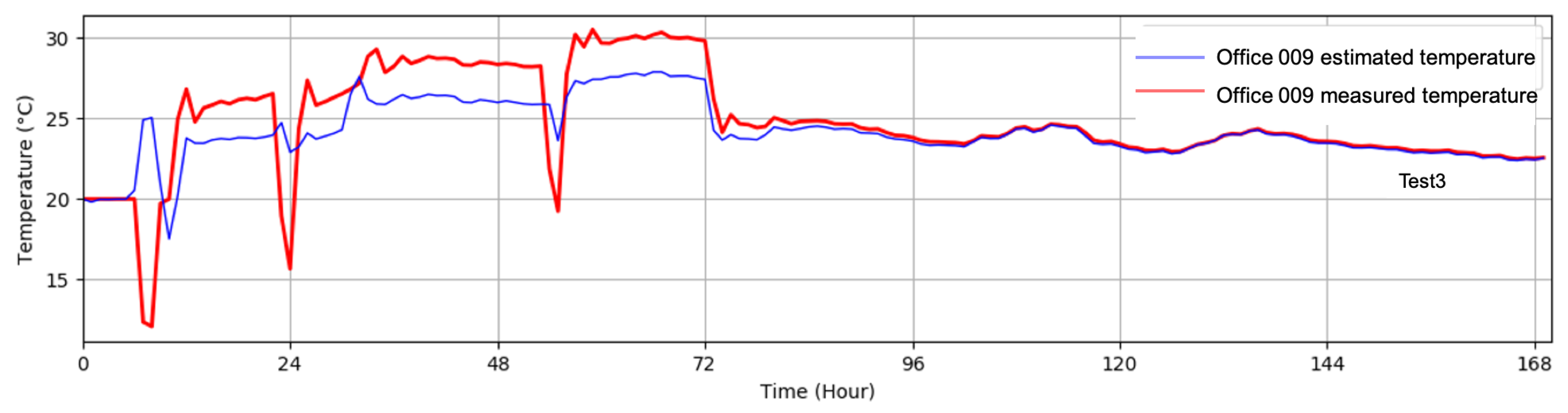
4.3. Test3 (Zonal Thermal Test), Model-Based

A simplified model is used for estimating the indoor temperature ($T_{est}$). Simplified models are easy to initialize due to fewer parameters and only account for zonal properties [24]. Estimated temperature $\left(T_{est}\right)$ is compared with the measured temperature ($T_{measured}$) and $\Delta T$ is a small value. Likewise, like rule- and range-based tests, model-based tests must also satisfy the behavioral and validity constraints. For this test, possible explanations are obtained from the modeled component in considering the model.

Modal-based zonal test:

$$\mathbf{Test}\mathbf{3}\left(T_{est}\right)=\left\{\begin{array}{cc}inconsistent\hfill & if\left(\neg (K\left(X_{(t,t+h)}\right)\in D_k)\wedge V\left(X_{(t,t+h)}\right)\in D_v)\right)\hfill \\ consistent\hfill & if\left((K\left(X_{(t,t+h)}\right)\in D_k)\wedge V\left(X_{(t,t+h)}\right)\in D_v)\right)\hfill \\ noconclusion\hfill & otherwise\hfill \end{array}\right.$$

(3)

where

$$\begin{array}{cc}\hfill K(X_{(t,t+h)}\in D_k)& \to (T_{measured}-\Delta T\le \left(T_{est}\right))\wedge (obs\left(T_{in}\right)\le T_{measured}+\Delta T)\hfill \\ \hfill V(X_{(t,t+h)}\in D_v)& \to (obs\left(occupancy\right)\in (occupanc{y}_{min},occupanc{y}_{max})\hfill \\ & \wedge (T_{out}\in \left(T_{min}^{weatherpredicted},T_{max}^{weatherpredicted}\right)\hfill \\ & \wedge \left(obs\right(doororwindowposition)\in (close,open)\hfill \end{array}$$

Possible fault explanations for Test3:

open door or window ∨ inefficient ventilation system ∨ inefficient heating system ∨ unplanned appliances ∨ misconfigured or faulty BEMS.

Required sensors for validity:

• $obs\left(occupancy\right):\mathrm{estimated}\mathrm{based}\mathrm{on}\mathrm{power}\mathrm{consumption}\mathrm{and}\mathrm{indoor}{\mathrm{CO}}_2\mathrm{level}$
• $obs\left(T_{out}\right):\mathrm{outdoor}\mathrm{sensor}\mathrm{reading}$
• $obs\left(doororwindowposition\right):\mathrm{contact}\mathrm{sensor}$

Required sensors for behavior:

• $obs\left(T_{in}\right):\mathrm{indoor}\mathrm{temperature}\mathrm{sensor}\mathrm{reading}$
• $obs\left(occupancy\right):\mathrm{estimated}\mathrm{based}\mathrm{on}\mathrm{power}\mathrm{consumption}\mathrm{and}\mathrm{indoor}{\mathrm{CO}}_2\mathrm{level}$
• $obs\left(T_{out}\right):\mathrm{outdoor}\mathrm{sensor}\mathrm{reading}$
• $obs\left(doororwindowposition\right):\mathrm{contact}\mathrm{sensor}$

Assumption:

Sensors used for behavioral and validity constraints are in $okstate$.

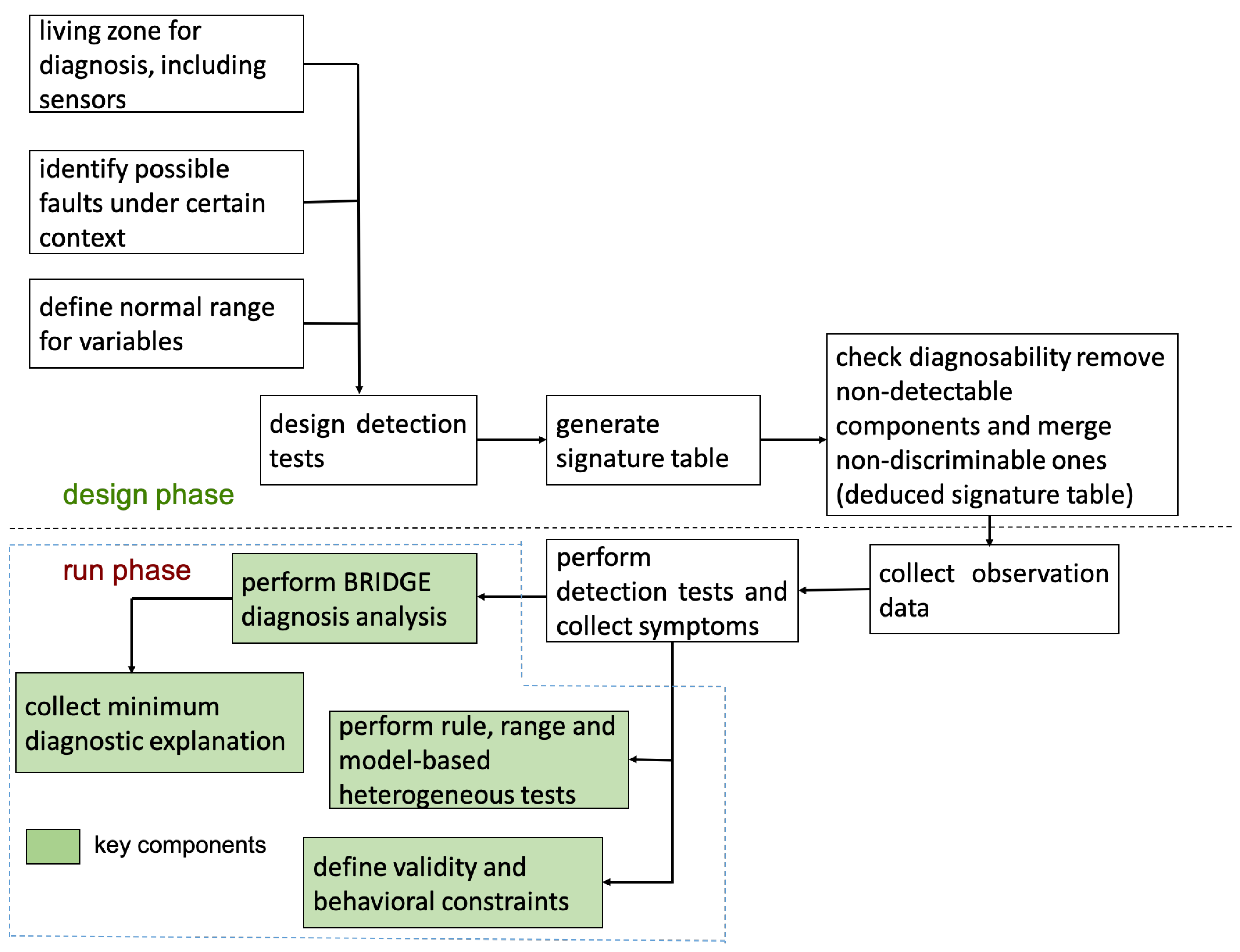
5. Analyzing Heterogeneous Tests

In practice, two diagnosis approaches have been widely adopted. The first is fault detection and isolation (FDI) supported by the control community [25] and focuses on model-based testing exclusively. FDI assumes abnormality in modeled behavior, which implies faults in the system. The second is inspired from artificial intelligence and known as logical diagnosis (DX) [26,27]. The DX approach mainly deals with the static system and adopts consistency-based diagnosis (CBD). DX assumes that faulty behavior cannot be determined only by behavior; it should involve components. In recent scientific literature, the importance of component-level analysis applied to a complex system to improve decision-making is explained in [28,29]. Moreover, multiple fault diagnosis is also a challenging task for FDI, though DX can deal with it easily.

To deal with the limitations of FDI and DX approaches, a group of contemporary researchers [18,30,31] have proposed a BRIDGE (FDI and DX) approach. The BRIDGE is applicable for both static and dynamic systems under certain conditions. The mainstay of the BRIDGE approach is the capability of finding a diagnosis with a component-level explanation.

In the present application, a logic-based BRIDGE [18,32] with formal diagnosis is used for diagnoses analysis. An example of logical reasoning for $Test$ is given below:

$$\mathbf{Test}=\left\{\begin{array}{cc}consistent\left(0\right)\hfill & if:\left((K\left(X_{(t,t+h)}\right)\in D_k)\wedge V\left(X_{(t,t+h)}\right)\in D_v)\right)\hfill \\ inconsistent\left(1\right)\hfill & if:\left(\neg (K\left(X_{(t,t+h)}\right)\in D_k)\wedge V\left(X_{(t,t+h)}\right)\in D_v)\right)\hfill \\ noconclusion\hfill & otherwise\hfill \end{array}\right.$$

(4)

where ∧ is a logical AND operator with K and V as behavioral and validity constraints, respectively. BRIDGE uses the notion of normalized Hamming distance ($d_H$) (Definition 8) and the possible diagnosis explanation [18]. Moreover, it is assumed that an absence of symptoms does not imply an absence of defect. However, a restoration event such as a window closing could occur while performing the test over a batch of data. BRIDGE explicitly uses the diagnosis based on the row analysis of the signature table.

Diagnoses Explanation

All possible explanations from rule-, range-, and model-based tests are merged into a single fault-signature table for further analysis. It is a tabular representation of faults in the form of tests with (0) and (1) where (1) means a fault is potentially detected for the related test, otherwise (0). This table can be obtained from cause–consequence analysis between system component and linked test.

To explain the proposed approach, a short and concrete example is chosen below. Consider the following signature table that combines rule-, range-, and model-based test explanations. Furthermore, range-, rule-, and model-based tests are performed over the set of data. This set of data consists of behavioral and validity data for the tested variable.

Furthermore, the test result (Equation (5)) i.e., symptoms coming from above three tests are inconsistent (represented by 1):

$$\begin{array}{cc}\hfill \left[\begin{array}{c}Test1\\ Test2\\ Test3\end{array}\right]& =\left[\begin{array}{c}1\\ 1\\ 1\end{array}\right]\hfill \end{array}$$

(5)

This symptom could be explained in terms of a combination of non-zero elements in each row of the signature

Table 2. Deduced signature table form all possible explanations.

Test	not ok(ventilation system)	not ok(heating system)	not ok(duct)	not ok(boiler)
$Test1$ (range-based) (Equation 1)	1	1	1	1
$Test2$ (rule-based) (Equation 2)	1	0	1	0
$Test3$ (model-based) (Equation 3)	1	1	0	0

1 = not ok (component), 0 = ok (component).

. The conventional column-based diagnoses approach such as FDI could detect only a ventilation system as a fault. In contrast to FDI, the BRIDGE approach develops a row-based test Explanation for each inconsistent test. Furthermore, a possible explanation for the above symptoms could be given as:

$$\begin{array}{cc}\hfill Expl\left(Test1\right)& =notok\left(ventilationsystem\right)\vee notok\left(heatingsystem\right)\vee notok\left(duct\right)\vee notok\left(boiler\right)\hfill \\ \hfill Expl\left(Test2\right)& =notok\left(ventilationsystem\right)\vee notok\left(duct\right)\hfill \\ \hfill Expl\left(Test3\right)& =notok\left(ventilationsystem\right)\vee notok\left(heatingsystem\right)\hfill \end{array}$$

These explanations are considered to be all possible sets of conflicts that could be responsible for the related faults. A Hitting set algorithm (Definition 7) described in [26], could be used for conflict analysis, which is depicted in Figure 3.

Definition 7.

(Hitting set) A hitting set H for the $ok\left(Componentsstats\right)=\left\{c_1,c_2,c_3....c_n\right\}\subseteq \mathit{ok}\left(\mathit{COMPONENTS}\right)$ if $H\subseteq U_{1\le k\le n}{c}_n$, and $H\cap c_n\ne \left\{\right\}$. Set H is minimal if and only if $\forall X\subset H,X$ is not a Hitting set.

Definition 8.

(Normalized Hamming distance) For given two equal-length binary vectors $b_1$ and $b_2$, normalized Hamming distance $d_H$ is defined as $d_H(b_1,b_2)=($bit-wise changes in $b_1$ and $b_2$) / (number of bits in $b_1$ or $b_2$).

To follow a fault-isolation process, normalized Hamming distance measures the closeness between the observed symptom and each column of Table 2. Knowing that Test1, Test2, and Test3 are giving faulty results (Equation (5)), the normalized Hamming distance ($d_H$) is given below. This distance is computed between the observed signature (Equation (5)) and each column of Table 2.

$$\begin{array}{c}\hfill d_H\left(notok\left(ventilationsystem\right)\right)=0\\ \hfill d_H\left(notok\left(heatingsystem\right)\right)=0.33\\ \hfill d_H\left(notok\left(duct\right)\right)=0.33\\ \hfill d_H\left(notok\left(boiler\right)\right)=0.66\end{array}$$

Using Hamming distance analysis, it is very obvious that $notok\left(ventilationsystem\right)$ is a declared fault because it is closer to the first column in the test signature table. However, the bridge method goes to the next level of analysis based on test explanations and tries to find a minimum possible explanation for all faults. Also, ventilation is present in all test explanations marked as green, i.e., diagnosed in the beginning of HS-tree (Figure 3). Now, the other nodes follow an expansion considering the next set of explanation.

In Figure 3, nodes with green labels show the diagnosed $component$, while the nodes in the red represent the termination or blocked diagnosis process so that no additional work is required. The following equation shows the set diagnosed component achieved from Figure 3.

$$\begin{array}{cc}\hfill \mathit{Minimum}\mathit{diagnostic}\mathit{Explanation}& =notok\left(ventilationsystem\right)\hfill \\ & \wedge \left(\right(notok\left(heatingsystem\right)\vee notok\left(duct\right))\hfill \end{array}$$

In this example, diagnosis detects the problem in the ventilation, duct, and heating system. Hence, it will be easy to detect multiple faults in one diagnostic explanation.

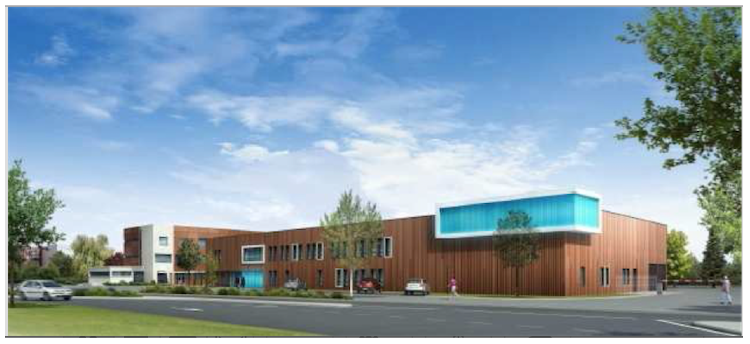
6. An Application of Proposed Methodology for Center for Studies and Design of Prototypes (CECP) Building

In this section, a case study is presented to discuss the diagnosability issue in the so-called center for studies and design of prototypes (CECP) building, which is an energy-efficient building constructed in 2012 and located in Angers, France. The building has one floor, and about 20 rooms. The whole building is divided into 74 zones with two major parts, namely a workshop area of 700 m² and an office area of 1000 m². About 30 people work in this building.

CECP follows the French energy efficiency building code RT-2005 for heating, cooling, ventilation, hot water supply, and lighting. According to the French building code, its energy consumption is labeled as 55.33 kWh/m²/year for the workshop area and 55.59 kWh/m²/year for the office area, respectively. A 3D view of the CECP building is shown in Figure 4. Each zone in the building is different from the other in terms of temperature and comfort requirement.

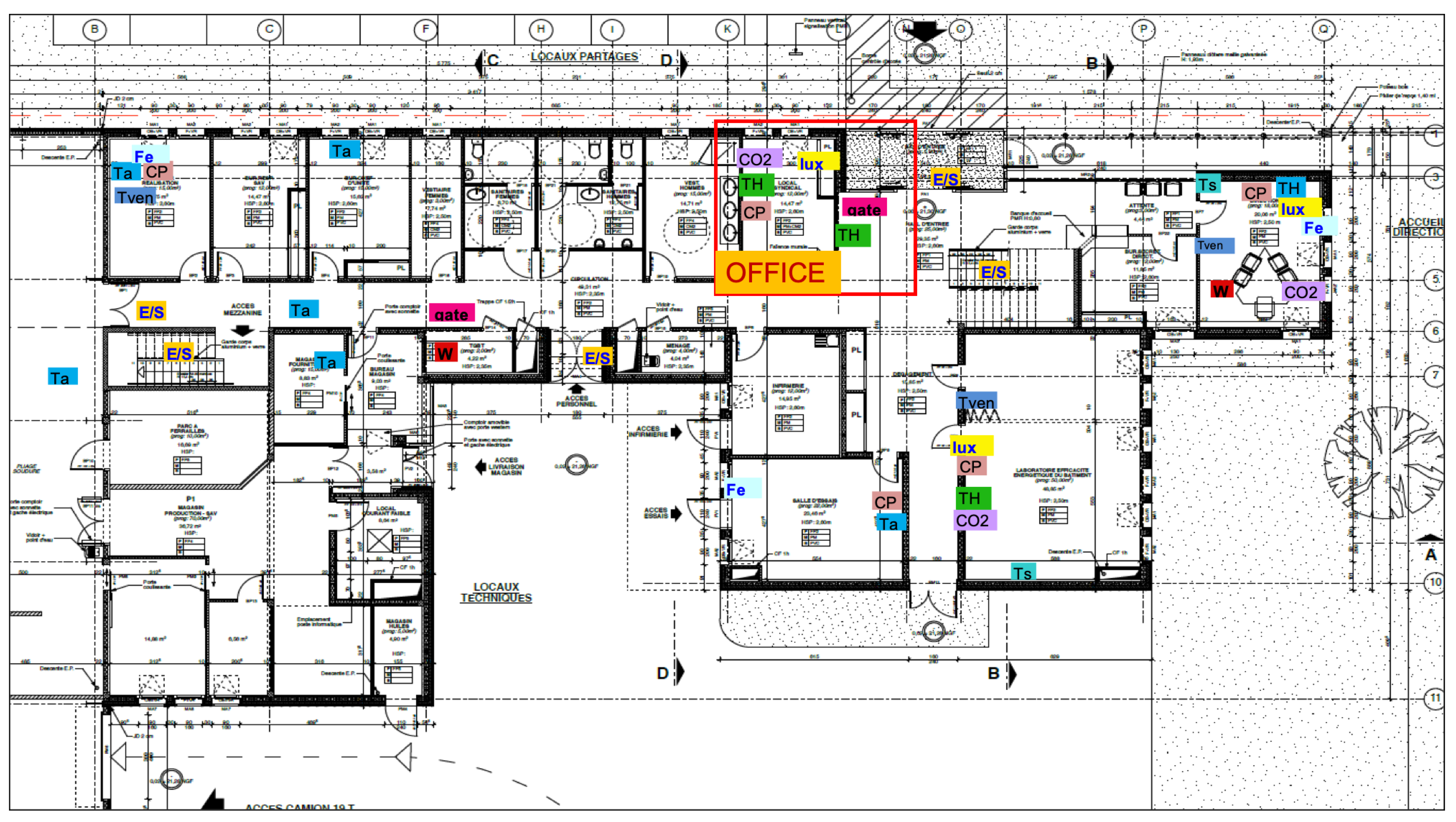
6.1. CECP Building Instrumentation

To monitor the CECP building, the following measuring points have been installed (Figure 5).

• on-site weather station (temperature, relative humidity, horizontal radiation, wind speed, and direction)
• ambient indoor temperatures in most rooms of the building (Ta); some sensors can also measure humidity (TH)
• heat energy in the boiler room for each outlet (for low-temperature radiators in the office area, etc.)
• electrical energy (W) for each differential circuit breaker to separate (lighting consumption, consumption of office outlets, consumption of auxiliaries etc.)
• motion detectors in most of the offices (CP)
• CO₂ concentration sensors in the corridors, in the meeting rooms, and in some offices.
• passage detectors at the entrances and exits of the building (E/S)
• some surface temperatures (Ts) sensors
• most of the offices are equipped with luxmeters

6.2. ARX (Auto Regressive) Thermal Model

An ARX model with exogenous input has been used to model the normal and fast dynamic behaviors of the CECP building. This is a simple-to-implement thermal model without deep mathematical knowledge of the building system under study. Moreover, this model neither takes into account the existing links between parameters nor the physical relationships between variables. The building energy simulation divides the office part into 74 thermal zones. Each zone in the building is different from the other in terms of temperature and comfort requirement. The inputs of the simulation correspond to measurements that were made in 2015:

• indoor temperature is the one that has been measured in each zone
• internal gains come from measured electrical appliances (global measurement)
• meteorological conditions that have been measured on site

The model takes into account parameters that have not been measured, for example:

• human presence.

Parameter identification:

Model parameters are estimated by the least-squares identification to minimize the error between estimation and measurements [33,34]. Two sets of separated data set between January 2015 and December 2015 have been used for the estimation and validation process. All inputs are measured on site, and output of the model is estimated with the help of Equation (6).

Mathematical representation:

$$\begin{array}{c}\hfill T\left[k\right]=0.226378T[k-1]-0.002148U_0\left[k\right]+0.052236U_1\left[k\right]-0.000062U_2\left[k\right]\\ \hfill +0.000029U_3\left[k\right]-0.000228U_4\left[k\right]+0.012467U_5\left[k\right]-0.656953U_6\left[k\right]\\ \hfill -0.450027U_7\left[k\right]+0.450887U_8\left[k\right]+0.283410U_9\left[k\right]\\ \hfill +0.423809U_{10}\left[k\right]+0.020218\end{array}$$

(6)

Input:

• $U_0=T_{ext}:$ Outdoor temperature
• $U_1=T_{corridor}:$ Air temperature in the corridor
• $U_2=W_{electrical}:$ Electrical consumption in office 009
• $U_3=Q_{horizontal}:$ The horizontal radiation
• $U_4=Airflow:$ Airflow in the office 009
• $U_5=T_{vent}:$ Temperature of air blown in the office 009
• $U_6=Q_{radiator}:$ Radiator heat flow
• $U_7=T_{office101}:$ Air temperature in neighboring office 101
• $U_8=T_{office010}:$ Air temperature in neighboring office 010
• $U_9=T_{atel-prod}:$ Air temperature in the room ATEL-PROD
• $U_{10}=$ Occupancy in office 009

Output:

• $T=T_{office009}$ Output estimated temperature in office 009

Sensitivity analysis:

The goal of the sensitivity analysis is to highlight critical parameters for building performance. These are parameters whose values have a great influence on the model result. The implementation of a performance contract could therefore contain a clause concerning these parameters. Morris method is used to perform the sensitivity analysis. The objective here is not to precisely know the value of the effects of each parameter, but rather to rank or even select the most influential parameters. The standard deviation of the associated elementary effects is also calculated in the following table (

Table 3. Sensitivity analysis for important parameter.

Uncertain Parameters	Low Level	Average	Standard Deviation
indoor temperature ($T_{in}$)	$-2$ K	20.7 °C	$+2$ K
number of occupants	$-60\%$	average profile	$+60\%$
internal gain from occupants	$-50\%$	8 W/m2 per occupation	$+50\%$
outdoor temperature	$-2$ K	weather norm	$+2$ K
horizontal solar radiation	$-50\%$	weather norm	$-50\%$

). Each parameter is associated with a high and a low value defining a range of uncertainty chosen by an expert and/or by comparison with the scientific literature.

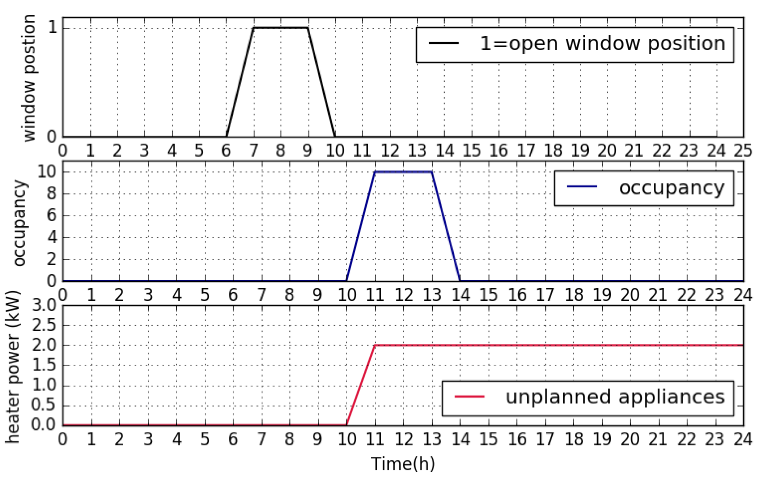
6.3. Simulated Fault Scenario

TRNsys (simulation software) with interface TRNBuild and TRNsys Simulation Studio (graphical front-end) have been used to simulate the building faults. TRNBuild interface allows adding the non-geometrical properties such as wall and layer material properties, window and door properties, thermal conductivity and different gains etc. In the present work, these values are taken from the French building code.

Table 4. Simulated fault scenario.

Hour	Simulated Fault	Data Set Used
0–1	-
1–2	-
2–3	-
3–4	-
4–5	-
5–6	-
6–7	window is open	Batch 1
7–8	window is open
8–9	window is open
9–10	window is open
10–11	unplanned appliances, unplanned occupancy
11–12	unplanned appliances, unplanned occupancy
12–13	unplanned appliances, unplanned occupancy	Batch 2
13–14	unplanned appliances, unplanned occupancy
14–15	unplanned appliances
15–16	unplanned appliances
16–17	unplanned appliances
17–18	unplanned appliances
18–19	unplanned appliances	Batch 3
19–20	unplanned appliances
20–21	unplanned appliances
21–22	unplanned appliances
22–23	unplanned appliances
23–24	unplanned appliances

and Figure 6 show the simulated fault scenario over a data set, namely Batch 1, Batch 2, and Batch 3, for a 24-hour duration.

Faults are simulated by adding or tuning different parameters in the fault model. The detail of simulated faults is given below:

• open window: using a TRNsys model
• unplanned occupancy: considered to be abnormal occupancy, i.e., a large number of occupants are more present than allowed. In this scenario 10 occupants are considered; however, the usual occupancy is 4
• unplanned appliances: use of additional appliances, causing internal heat gain and over-consumption. In the present case study, a heater of 2 kW/h is simulated as the unplanned appliance

6.4. Tests Analysis for (CECP) Building

In this case study, only the thermal performance of the building has been tested. The range and model-based tests are proposed in Section 4.1 and Section 4.3. A range-based thermal test confirms a thermal discomfort and symptom manifest when the indoor temperature goes beyond the comfort boundary, i.e., 18 °C ($T_{min}$) and 22 °C ($T_{max}$).

Figure 7 shows thermal discomfort is detected between the hours of 6 to 169. Beyond the maximum and minimum temperature range, a building enters the thermal discomfort zone. This test confirms the discrepancy in the building’s normal thermal performance.

An ARX model-based zonal test is used to test the thermal performance at the zonal level. A model-based zonal test (Section 4.3) is used to verify the zonal temperature. This test performs a comparison of the measured and estimated temperature. The thermal model verifies the thermal discomfort at the zonal or local level. This test yields the set-point deviation symptom along with the thermal discomfort. Figure 8 shows the measured and estimated temperature value.

The zonal test is performed with the help of the linear regression model (Equation (6)) [33]. It compares whether the measurements follow the estimated temperatures or not. However, zonal temperature can adjust $\pm \Delta T^{\circ }C=2^{\circ }C$.

Moreover, the following set of validity constraints are used to analyze the test validity.

$$\begin{array}{cc}\hfill V(X_{(t,t+h)}\in D_v)& \to (obs\left(occupancy\right)\in (occupanc{y}_{min},occupanc{y}_{max})\hfill \\ & \wedge \left(obs\right(windowposition)\in (close,open)\hfill \end{array}$$

These constraints verify the window position and occupancy level (Figure 6).

6.5. Symptoms Analysis for CECP Building

This section demonstrates the experimental validation of the proposed diagnosis methodology. The tests were performed for the different building zones which include several offices and meeting rooms. Tests are derived from the one-week data collection from the CECP building. To make a concise explanation only the first 24-hours i.e., one day with three different scenarios and data set (Batch 1,2 &3), are accounted for in the fault analysis.

Table 5. Validity and behavioral constraints for tests.

Hour	Test1 ( Equation 1)	Test3 ( Equation 3)	Conclusion (Test1)	Conclusion (Test3)
0–1	$K=0$, $V=0$	$K=0$, $V=0$	$consistent$	$consistent$
1–2	$K=0$, $V=0$	$K=0$, $V=0$	$consistent$	$consistent$
2–3	$K=0$, $V=0$	$K=0$, $V=0$	$consistent$	$consistent$
3–4	$K=0$, $V=0$	$K=0$, $V=0$	$consistent$	$consistent$
4–5	$K=0$, $V=0$	$K=0$, $V=0$	$consistent$	$consistent$
5–6	$K=0$, $V=0$	$K\ne 0$, $V=0$	$consistent$	$inconsistent$
6–7	$K\ne 0$, $V\ne 0$	$K\ne 0$, $V=0$	$\mathit{noconclusion}$	$inconsistent$
7–8	$K=0$, $V\ne 0$	$K=0$, $V=0$	$\mathit{no}\mathit{conclusion}$	$inconsistent$
8–9	$K=0$, $V\ne 0$	$K\ne 0$, $V=0$	$\mathit{noconclusion}$	$inconsistent$
9–10	$K=0$, $V\ne 0$	$K\ne 0$, $V=0$	$\mathit{noconclusion}$	$inconsistent$
10–11	$K\ne 0$, $V=0$	$K\ne 0$, $V=0$	$inconsistent$	$inconsistent$
11–12	$K\ne 0$, $V=0$	$K\ne 0$, $V=0$	$inconsistent$	$inconsistent$
12–13	$K\ne 0$, $V=0$	$K\ne 0$, $V=0$	$inconsistent$	$inconsistent$
13–14	$K\ne 0$, $V=0$	$K\ne 0$, $V=0$	$inconsistent$	$inconsistent$
14–15	$K\ne 0$, $V=0$	$K\ne 0$, $V=0$	$inconsistent$	$inconsistent$
15–16	$K\ne 0$, $V=0$	$K\ne 0$, $V=0$	$inconsistent$	$inconsistent$
16–17	$K\ne 0$, $V=0$	$K\ne 0$, $V=0$	$inconsistent$	$inconsistent$
17–18	$K\ne 0$, $V=0$	$K\ne 0$, $V=0$	$inconsistent$	$inconsistent$
18–19	$K\ne 0$, $V=0$	$K\ne 0$, $V=0$	$inconsistent$	$inconsistent$
19–20	$K\ne 0$, $V=0$	$K\ne 0$, $V=0$	$inconsistent$	$inconsistent$
20–21	$K\ne 0$, $V=0$	$K\ne 0$, $V=0$	$inconsistent$	$inconsistent$
21–22	$K\ne 0$, $V=0$	$K\ne 0$, $V=0$	$inconsistent$	$inconsistent$
22–23	$K\ne 0$, $V=0$	$K\ne 0$, $V=0$	$inconsistent$	$inconsistent$
23–24	$K\ne 0$, $V=0$	$K\ne 0$, $V=0$	$inconsistent$	$inconsistent$

represents the test results in three different scenarios. Conclusions from Table 5 are:

• there is no inconsistency between the hours 0 and 5 which confirms the normal building operation.
• during the hours 5–6 only Test3 is inconsistent.
• in the period 6–10 Test1 shows no conclusion due to an open window in the morning.
• finally, all tests demonstrate inconsistency in building performance during the 10 to 24.

6.6. Heterogeneous Tests Analysis and Diagnosis Result

To simplify the approach, office room 009 of CECP building has been chosen for the diagnosis analysis. A few building components such as ventilation pipes, radiator, BEMS, etc. are considered to be possible test explanations. A heterogeneous test signature table below is developed, considering the range and model-based test.

Test explanations are computed from the all possible explanations given in

Table 6. Heterogeneous test signature table CECP building.

Test	$\mathit{n}\mathit{o}\mathit{t}\mathit{o}\mathit{k}(\mathit{f}\mathit{i}\mathit{l}\mathit{t}\mathit{e}\mathit{r}\vee \mathit{r}\mathit{a}\mathit{d}\mathit{i}\mathit{a}\mathit{t}\mathit{o}\mathit{r}$	$\mathit{n}\mathit{o}\mathit{t}\mathit{o}\mathit{k}(\mathit{v}\mathit{e}\mathit{n}\mathit{t}\mathit{i}\mathit{l}\mathit{a}\mathit{t}\mathit{i}\mathit{o}\mathit{n}\vee \mathit{B}\mathit{E}\mathit{M}\mathit{S}$	$\mathit{n}\mathit{o}\mathit{t}\mathit{o}\mathit{k}(\mathit{o}\mathit{c}\mathit{c}\mathit{u}\mathit{p}\mathit{a}\mathit{n}\mathit{c}\mathit{y}\vee$
	$\vee \mathit{pipes})$	$\vee \mathit{appliances})$	$\mathit{door}\mathit{or}\mathit{window}\mathit{position})$
$Test1$ (range-based) (Equation 1)	1	0	1
$Test3$ (model-based) (Equation 3)	0	1	1

1 = not ok (component), 0 = ok (component).

. These explanations have conflicting components and require further analysis.

$$\mathbf{Scenario}\mathbf{1}$$

Hour (0–5)

• Simulated fault: no fault has been simulated
• Detected symptom

  $$\begin{array}{cc}\hfill \left[\begin{array}{c}Test1\\ Test3\end{array}\right]& =\left[\begin{array}{c}0\\ 0\end{array}\right]\to \left(\mathrm{consistent}\mathrm{test}\mathrm{result}\right)\hfill \end{array}$$

In this duration, both tests are consistent and satisfy the behavioral and validity constraints. No inconsistency is revealed.

Hour (5–6)

• Simulated fault: no fault has been simulated
• Detected symptom

  $$\begin{array}{cc}\hfill \left[\begin{array}{c}Test1\\ Test3\end{array}\right]& =\left[\begin{array}{c}0\\ 1\end{array}\right]\to \left(\mathrm{consistent}\mathrm{and}\mathrm{inconsistent}\mathrm{test}\mathrm{result}\right)\hfill \end{array}$$

In this hour, only Test3 shows inconsistency. That confirms a zonal thermal discomfort. The test explanation for this test is given below:

$$\begin{array}{c}\hfill Expl\left(Test3\right)=notok(ventilation\vee BEMS\vee appliances)\\ \hfill \wedge notok(occupancy\vee doororwindowposition)\end{array}$$

The fault explanation shows the problem could be an open window or unplanned occupancy. Also, poor or faulty ventilation system, wrongly configured BEMS, and unplanned appliances could be a considerable fault. Indeed, there is no simulated fault in this hour. So far, at this stage it is difficult to say what is the reason behind this inconsistency.

$$\mathbf{Scenario}\mathbf{2}$$

Hour (6–10)

• Simulated fault: open window
• Detected symptom

  $$\begin{array}{cc}\hfill \left[\begin{array}{c}Test1\\ Test3\end{array}\right]& =\left[\begin{array}{c}noconclusion\\ 1\end{array}\right]\to \left(\mathrm{no}\mathrm{conclusion}\mathrm{and}\mathrm{inconsistent}\mathrm{test}\mathrm{result}\right)\hfill \end{array}$$

During the hours 6–10, Test1 shows no conclusion because of opening of the window and not considered for further analysis. However, Test3 is still inconsistent, which means the fault is still present in the system. The Test explanation is same as the previous scenario.

$$\begin{array}{c}\hfill Expl\left(Test3\right)=notok(ventilation\vee BEMS\vee appliances)\\ \hfill \wedge notok(occupancy\vee doororwindowposition)\end{array}$$

However, compared to the simulated fault scenario, the obvious reason behind this fault is $notok\left(doororwindowposition\right)$. The actual fault scenario is the open window. Diagnosis analysis detects this fault along with other faults.

$$\mathbf{Scenario}\mathbf{3}$$

Hour (10–24)

• Simulated fault: unplanned appliances, unplanned occupancy
• Detected symptom

  $$\begin{array}{cc}\hfill \left[\begin{array}{c}Test1\\ Test3\end{array}\right]& =\left[\begin{array}{c}1\\ 1\end{array}\right]\to \left(\mathrm{inconsistent}\mathrm{test}\mathrm{result}\right)\hfill \end{array}$$

In this duration, both tests show inconsistencies and a conflicting situation arising in the diagnosis. Therefore, the Hamming distance between observed symptom and Table 6 is give below:

$$\begin{array}{c}\hfill d_H\left(notok(filter\vee radiator\vee pipes)\right)=0.5\\ \hfill d_H\left(notok(ventilation\vee BEMS\vee appliances)\right)=0.5\\ \hfill d_H\left(notok(occupancy\vee doororwindowposition)\right)=0\end{array}$$

Test explanations are:

$$\begin{array}{cc}\hfill Expl\left(Test1\right)& =notok(filter\vee radiator\vee pipes)\wedge notok(occupancy\vee doororwindowposition)\hfill \\ \hfill Expl\left(Test3\right)& =notok(ventilation\vee BEMS\vee appliances)\wedge notok(occupancy\vee doororwindowposition)\hfill \end{array}$$

Furthermore, bridge diagnosis analysis finds the following faults as possible diagnosis:

$$\begin{array}{cc}\hfill \mathit{Minimum}\mathit{diagnostic}\mathit{ExplAnation}=& notok(occupancy\vee doororwindowposition)\hfill \\ & \wedge \left(notok\right(filter\vee radiator\vee pipes)\hfill \\ & \vee notok(ventilation\vee BEMS\vee appliances))\hfill \end{array}$$

BRIDGE analyzes both test explanations and most reasonable issues are occupancy and building openings, i.e., door or window open. This confirms that faults with open window are still present in the system.

The simulated fault in this scenario is unplanned appliances and unplanned occupancy. BRIDGE diagnosis confirms that at least one of the combinations, i.e., ($occupancy\vee doororwindow$) is faulty. However, the other simulated fault, unplanned appliance, is detected with faulty $notok(ventilation\vee BEMS\vee appliances)$, i.e., the issue with the ventilation system, unplanned appliances or failure of BEMS.

Furthermore, the diagnosis is terminated with at least two combinations of minimal diagnoses, which are:

$$\begin{array}{c}\hfill notok(occupancy\vee doororwindowposition)AND\\ \hfill notok(filter\vee radiator\vee pipes)\vee notok(ventilation\vee BEMS\vee appliances)\end{array}$$

Diagnosis results are illustrated in Figure 9. The results have proved that at least one of these combinations must be faulty. In conclusion, the proposed diagnosis approach can detect simulated faults with validity under the single and multiple fault scenarios. At the same time, the minimum diagnosis explanation addresses the all possible faults and reduces the further search process.

7. Conclusions

The advantage of providing a building diagnostic system based on contextual tests and consistency analysis are three-fold. First, the validity of diagnosed fault can be verified easily. Proposed contextual tests are valid under certain contexts and relatively easy to apply under real building conditions. Second, the knowledge from heterogeneous tests can be combined into one fault diagnosis analysis. This scales down the whole-building fault modeling effort. Lastly, a minimum set of possible faulty components is derived from the consistency analysis method. Such explanations allow an easy fault-isolation process. The results show that the proposed methodology can diagnose multiple fault scenarios. Given the set of minimum explanations, a facility manager can determine what may be wrong with the building system being diagnosed. The limitation of the proposed contextual and heterogeneous tests is that they rely on an assumption i.e., non-faulty sensors and actuators. Moreover, a faulty sensor or measurement could disturb the applicability of the proposed methodology. The future of the proposed work is to develop a comprehensive whole-building fault-analytics tool that could incorporate sensor failures. Also, future work will focus on designing of different test at component level and sub-component level. We are willing to extend our approach for developing an interactive building fault diagnosis tool combining the domain expert knowledge and experience.

References

1. Calvillo, F.C.; Sánchez-Miralles, A.; Villar, J. Energy management and planning in smart cities. J. Renew. Sustain. Energy Rev. 2017, 55, 273–287. [Google Scholar]
2. Le, M.; Ploix, S.; Wurtz, F. Application of an anticipative energy management system to an office platform. In Proceedings of the BS 2013—13th Conference of the International Building Performance Simulation Association, Chambéry, France, 26–28 August 2013. [Google Scholar]
3. Katipamula, S.; Brambley, M.R. Review article: Methods for fault detection, diagnostics, and prognostics for building systems, Part I. Hvac&R Res. 2005, 11, 3–26. [Google Scholar]
4. Katipamula, S.; Brambley, M.R. Review article: Methods for fault detection, diagnostics, and prognostics for building systems, Part II. Hvac&R Res. 2005, 11, 169–187. [Google Scholar]
5. Lazarova-Molnar, S.; Shaker, R.H.; Mohamed, N.; Jørgensen, N.B. Fault detection and diagnosis for smart buildings: State of the art, trends and challenges. In Proceedings of the 3rd MEC International Conference on Big Data and Smart City (ICBDSC), Muscat, Oman, 15–16 March 2016; pp. 1–7. [Google Scholar]
6. Wang, S.; Yan, C.; Xiao, F. Quantitative energy performance assessment methods for existing buildings. Energy Build. 2012, 55, 873–888. [Google Scholar] [CrossRef]
7. Derouineau, S.; Fouquier, A.; Mohamed, A.; Perehinec, A.; Couilladus, N. Specifications for Energy Management, Fault Detection and Diagnosis Tools. Technical Report: Prepared for the European Project PERFORMER. 2015, pp. 35–55. Available online: http://performerproject.eu/wp-content/uploads/2015/04/PERFORMER_D1-4_Specification-for-energy-management-FDD-Tools.pdf (accessed on 1 September 2015).
8. Du, Z.; Jin, X.; Yang, Y. Fault diagnosis for temperature, flow rate and pressure sensors in VAV systems using wavelet neural network. Appl. Energy 2009, 86, 1624–1631. [Google Scholar]
9. Li, S.; Wen, J. A model-based fault detection and diagnostic methodology based on PCA method and wavelet transform. Energy Build. 2014, 68, 63–71. [Google Scholar]
10. O’Neill, Z.; Pang, X.; Shashanka, M.; Haves, P.; Bailey, T. Model-based real-time whole building energy performance monitoring and diagnostics. J. Build. Perform. Simul. 2014, 7, 83–99. [Google Scholar] [CrossRef]
11. Najeh, H.; Singh, M.P.; Chabir, K.; Ploix, S.; Abdelkrim, N.M. Diagnosis of sensor grids in a building context: Application to an office setting. J. Build. Eng. 2018, 17, 75–83. [Google Scholar]
12. Schumann, A.; Hayes, J.; Pompey, P.; Verscheure, O. Adaptable Fault Identification for Smart Buildings. In Proceedings of the 7th AAAI Conference on Artificial Intelligence and Smarter Living: The Conquest of Complexity, San Francisco, CA, USA, 7–8 August 2011; pp. 44–47. [Google Scholar]
13. Oh, T.-K.; Lee, D.; Park, M.; Cha, G.; Park, S. Three-Dimensional Visualization Solution to Building-Energy Diagnosis for Energy Feedback. Energies 2018, 11, 1736. [Google Scholar] [CrossRef]
14. Dey, A.K. Understanding and Using Context. J. Pers. Ubiquitous Comput. 2001, 5, 4–7. [Google Scholar] [CrossRef]
15. Fazenda, P.; Carreira, P.; Lima, P. Context-based reasoning in smart buildings. In Proceedings of the First International Workshop on Information Technology for Energy Applications, Lisbon, Portugal, 6–7 September 2012; pp. 131–142. [Google Scholar]
16. Pardo, E.; Espes, D.; Le-Parc, P. A Framework for Anomaly Diagnosis in Smart Homes Based on Ontology. Procedia Comput. Sci. 2016, 83, 545–552. [Google Scholar] [CrossRef] [Green Version]
17. Singh, M. Improving Building Operational Performance with Reactive Management Embedding Diagnosis Capabilities. Ph.D. Thesis, Université Grenoble Alpes, Grenoble, France, 2017. [Google Scholar]
18. Ploix, S. Des systèmes automatisés aux systèmes coopérants application au diagnostic et á la gestion énergétique. In Habilitation à diriger des recherches (HDR); Grenoble-INP: Grenoble, France, 2009; Chapter 3 and 5; pp. 43–51. [Google Scholar]
19. Gentil, S.; Lesecq, S.; Barraud, A. Improving decision making in fault detection and isolation using model validity. Eng. Appl. Artif. Intell. 2009, 22, 534–545. [Google Scholar] [CrossRef]
20. Carli, R.; Dotoli, M.; Pellegrino, R. A Hierarchical Decision-Making Strategy for the Energy Management of Smart Cities. IEEE Trans. Autom. Sci. Eng. 2017, 14, 505–523. [Google Scholar] [CrossRef]
21. Carli, R.; Dotoli, M. Decentralized control for residential energy management of a smart users microgrid with renewable energy exchange. IEEE/CAA J. Autom. Sin. 2019, 6, 641–656. [Google Scholar] [CrossRef]
22. Hosseini, M.S.; Carli, R.; Dotoli, M. Model Predictive Control for Real-Time Residential Energy Scheduling under Uncertainties. In Proceedings of the 2018 IEEE International Conference on Systems, Man, and Cybernetics (SMC), Miyazaki, Japan, 7–10 October 2018; pp. 1386–1391. [Google Scholar]
23. Singh, M.; Ploix, S.; Wurtz, F. Handling Discrepancies in Building Reactive Management Using HAZOP and Diagnosis Analysis. In Proceedings of the ASHRAE 2016 Summer Conference, St. Louis, MI, USA, 25–29 June 2016; pp. 1–8. [Google Scholar]
24. Wang, S.; Xu, X. Simplified building model for transient thermal performance estimation using GA-based parameter identification. Int. J. Therm. Sci. 2006, 45, 419–432. [Google Scholar] [CrossRef]
25. Isermann, R. Model-based fault-detection and diagnosis—Status and applications. Ann. Rev. Control 2005, 29, 71–85. [Google Scholar] [CrossRef]
26. Reiter, R. A Theory of Diagnosis from First Principles. Artif. Intell. 1987, 32, 57–95. [Google Scholar] [CrossRef]
27. De Kleer, J.; Mackworth, A.K.; Reiter, R. Characterizing diagnoses and systems. Artif. Intell. 1992, 56, 197–222. [Google Scholar] [CrossRef] [Green Version]
28. Leszek, C.; Michal, T.; Bogusz, W. Multi-criteria Decision making in Components Importance Analysis applied to a Complex Marine System. J. Nase More 2016, 64, 264–270. [Google Scholar]
29. Leszek, C.; Katarzyna, G. Selected issues regarding achievements in component importance analysis for complex technical systems. Sci. J. Maritime Univ. Szczecin 2017, 52, 137–144. [Google Scholar]
30. Ploix, S.; Touaf, S.; Flaus, J.M. A logical framework for isolation in faults diagnosis. IFAC Proc. Vol. 2003, 36, 807–812. [Google Scholar] [CrossRef]
31. Cordier, M.O.; Dague, P.; Lévy, F.; Montmain, J.; Staroswiecki, M.; Travé-Massuyès, L. Conflicts versus analytical redundancy relations: A comparative analysis of the model based diagnosis approach from the artificial intelligence and automatic control perspectives in Systems, Man, and Cybernetics. Syst. Man Cybern. Part B Cybern. 2004, 34, 2163–2177. [Google Scholar] [CrossRef]
32. Zhang, W.; Zhao, Q.; Zhao, H.; Zhou, G.; Feng, W. Diagnosing a Strong-Fault Model by Conflict and Consistency. Sensors 2018, 18, 1016. [Google Scholar] [CrossRef] [PubMed]
33. Hoang, M.L.; Kien, T.N. Building thermal modeling using equivalent electric circuit: Application to the public building platform. Autom. Today 2015, 14, 26–33. [Google Scholar]
34. Ljung, L. System Identification: Theory for the User, 2nd ed.; Prentice Hall PTR: Upper Saddle River, NJ, USA, 1999. [Google Scholar]
Figure 1. Enumerated scheme of the proposed building diagnosis framework.
Energies 12 02510 g001
Figure 2. Behavioral and Contextual test for diagnosis.
Energies 12 02510 g002
Figure 3. Hitting Set (HS) tree.
Energies 12 02510 g003
Figure 4. 3D view of CECP Building.
Energies 12 02510 g004
Figure 5. Building plan and instrumentation.
Energies 12 02510 g005
Figure 6. Simulated fault scenario for office 009.
Energies 12 02510 g006
Figure 7. Range-based thermal test for thermal discomfort.
Energies 12 02510 g007
Figure 8. Model-based zonal thermal test for thermal discomfort in office 009.
Energies 12 02510 g008
Figure 9. HITTING SET (HS)-tree for diagnosed faults.
Energies 12 02510 g009