Sensitivity of Characterizing the Heat Loss Coefficient through On-Board Monitoring: A Case Study Analysis

Abstract

Recently, there has been an increasing interest in the development of an approach to characterize the as-built heat loss coefficient (HLC) of buildings based on a combination of on-board monitoring (OBM) and data-driven modeling. OBM is hereby defined as the monitoring of the energy consumption and interior climate of in-use buildings via non-intrusive sensors. The main challenge faced by researchers is the identification of the required input data and the appropriate data analysis techniques to assess the HLC of specific building types, with a certain degree of accuracy and/or within a budget constraint. A wide range of characterization techniques can be imagined, going from simplified steady-state models applied to smart energy meter data, to advanced dynamic analysis models identified on full OBM data sets that are further enriched with geometric info, survey results, or on-site inspections. This paper evaluates the extent to which these techniques result in different HLC estimates. To this end, it performs a sensitivity analysis of the characterization outcome for a case study dwelling. Thirty-five unique input data packages are defined using a tree structure. Subsequently, four different data analysis methods are applied on these sets: the steady-state average, Linear Regression and Energy Signature method, and the dynamic AutoRegressive with eXogenous input model (ARX). In addition to the sensitivity analysis, the paper compares the HLC values determined via OBM characterization to the theoretically calculated value, and explores the factors contributing to the observed discrepancies. The results demonstrate that deviations up to 26.9% can occur on the characterized as-built HLC, depending on the amount of monitoring data and prior information used to establish the interior temperature of the dwelling. The approach used to represent the internal and solar heat gains also proves to have a significant influence on the HLC estimate. The impact of the selected input data is higher than that of the applied data analysis method.

1. Introduction

With a share of 25.7% in the final energy consumption in the European Union [1], the residential sector has an important potential for the application of energy saving strategies such as increasing the energy efficiency, using renewable energy, and exchanging energy between buildings. In order to sensibly implement these strategies, thorough insight is required into three elements constituting the as-built energy performance of buildings: (1) the thermal performance of the building fabric, (2) the efficiency of the technical building systems, and (3) the behavior of the users. A key performance indicator to express the performance of the building envelope is the Heat Loss Coefficient or HLC (W/K). This metric describes the heating power (W) needed to sustain a temperature difference of 1K over the building envelope. As such, it is a combined measure of the thermal insulation quality and airtightness of the building fabric, as expressed in Equation (1) with H_tr the heat transfer coefficient by transmission (W/K) and H_inf the heat transfer coefficient by infiltration (W/K). The H_tr, on the one hand, embeds four separate heat transfer coefficients (Equation (2)): the heat transfer coefficient between the conditioned zone and the exterior environment (H_tr,e (W/K)), and the heat transfer coefficients to the ground (H_tr,g), to unconditioned spaces (H_tr,u) and to adjacent buildings (H_tr,a) [2]. All these terms (hence subscript ‘x’ in Equation (3)) can in turn be dissociated in the heat transfer through the (1) planar components, (2) linear thermal bridges, and (3) point thermal bridges. The building components are described by their surface area A (m²) and thermal transmittance or U-value (W/m²·K), the linear and point thermal bridges by, respectively, their length L (m) and linear thermal transmittance Ψ (W/m·K), and point thermal transmittance Χ (W/K). A temperature ratio b_T (-) ensures that all building fabric is evaluated over the temperature difference between the interior and exterior environment (Equation (4)). The H_inf on the other hand, can be expressed as the product of the density ρ_a (kg/m³) and specific heat capacity c_a (J/(kg K)) of the air and the infiltration flow rate Q_inf (m³/s) (Equation (2)).

$$\begin{array}{}\hfill \mathrm{(1)}& \begin{array}{cc}\hfill HL{C}_t& =H_{tr;t}+H_{inf;t}\hfill \end{array}\hfill \hfill \mathrm{(2)}& \begin{array}{cc}& =\left(H_{tr,e;t}+H_{tr,g;t}+H_{tr,u;t}+H_{tr,a;t}\right)+\left({\rho }_a·c_a·Q_{inf;t}\right)\hfill \end{array}\hfill \end{array}$$

$$H_{tr,x;t}=\left({\displaystyle \sum }_{i=1}^q\left(A_i·U_{i;t}\right)+{\displaystyle \sum }_{j=1}^r\left(L_j·{\mathsf{\Psi }}_{j;t}\right)+{\displaystyle \sum }_{k=1}^s{{\rm X}}_{k;t}\right)·b_{T,x;t}$$

(3)

$$b_{T,x;t}=\left(\left({\theta }_{x;t}-{\theta }_{i;t}\right)/\left({\theta }_{e;t}-{\theta }_{i;t}\right)\right)$$

(4)

In general, the HLC is theoretically calculated using Equations (1)–(4). Since the actual values of the considered variables are typically unknown, they are based on design or default values. Furthermore, the as-built envelope performance can be influenced by workmanship issues. As a consequence, this bottom-up approach may lead to theoretical HLC values that substantially deviate from the actual metric and contribute to the ‘performance gap’ [3,4,5,6]. In search for alternative approaches, several researchers have developed on-site measurement methods that are capable of assessing the actual, as-built envelope performance. These dedicated tests include the coheating test [7,8], the Short Term Energy Monitoring (STEM) using Primary and Secondary Term Analysis and Renormalization (PSTAR) technique [9,10], the Quick U-value of Building (QUB) test [11,12], and the In Situ Assessment of the Building EnveLope pErformances (ISABELE) method [13,14,15]. Both the experimental design of these tests and the data analysis methods applied afterwards take the single-zone heat balance (Equation 5) as a starting point. When written in its original dynamic form, this balance states that the interior temperature θ_i (°C) of a zone with effective heat capacity C_i (J/K) is influenced by the net heating power supplied by the heating system Φ_h (W), the internal heat gains Φ_int, the solar gains through the transparent parts of the building envelope Φ_sol, and the heat transfer through intended ventilation Φ_v, envelope air infiltration Φ_inf and transmission Φ_tr. Based on Equations (1) and (2), and ignoring the difference between air and equivalent temperatures [16], the latter two can be combined and written as the HLC times the difference between the reference interior and exterior temperature (Equation (6)).

$$\begin{array}{}\hfill \mathrm{(5)}& \begin{array}{cc}\hfill C_i·d{\theta }_i/dt& \hfill ={\Phi }_{h;t}+{\Phi }_{int;t}+{\Phi }_{sol;t}+{\Phi }_{v;t}+{\Phi }_{inf;t}+{\Phi }_{tr;t}\end{array}\hfill \mathrm{(6)}& \begin{array}{cc}& \hfill ={\Phi }_{h;t}+{\Phi }_{int;t}+{\Phi }_{sol;t}+{\Phi }_{v;t}+HL{C}_t·\left({\theta }_{e;t}-{\theta }_{i;t}\right)\end{array}\end{array}$$

$${\Phi }_{h;t}={\Phi }_{h,sys;t}·{\eta }_{h,sys;t}$$

(7)

$${\Phi }_{int;t}={\Phi }_{int,Occ;t}+{\Phi }_{int,Ap\&Li;t}+{\Phi }_{int,Wa;t}+{\Phi }_{int,HVAC;t}$$

(8)

$${\Phi }_{sol;t}={\displaystyle \sum }_{i=1}^n{\Phi }_{sol;i;t}={\displaystyle \sum }_{i=1}^n\left(g_{i;t}·A_{i;t}·I_{sol; i;t}\right)$$

(9)

$${\Phi }_{v;t}=H_{v;t}·\left({\theta }_{air,e;t}-{\theta }_{air,i;t}\right)={\rho }_a·c_a·{\displaystyle \sum }_{p=1}^r\left(Q_{V;p;t}·b_{v;p;t}\right)·\left({\theta }_{air,e;t}-{\theta }_{air,i;t}\right)$$

(10)

The net heating power Φ_h (Equation (7)) equals the energy use of the heating system Φ_h,sys times the overall system efficiency η_h,sys (-), which accounts for unrecoverable generation, storage, distribution, and emission losses. The internal heat flow rate Φ_int (Equation (8)) encompasses the heat flow rate from occupants (Φ_int,Occ) and appliances and lighting (Φ_int,Ap&Li), the heat dissipated from or absorbed by hot and mains water and sewage (Φ_int,Wa), and the recoverable losses to or from heating, cooling, and ventilation systems Φ_int,HVAC. The total solar gain of the zone, Φ_sol (Equation (9)), can be expressed as the sum of the solar gains through each of the n transparent elements of its envelope. The size of these gains is determined by (1) the g-value of the element’s glass panes (-); (2) the element’s effective area A (m²), which is the total surface area corrected by a frame area fraction and shading reduction factor; and (3) the combined direct and diffuse solar irradiance I_sol (W/m²) for a given orientation and inclination. Finally, the heat losses through intended ventilation Φ_v (Equation (10)) can be detailed as the product of the heat transfer coefficient H_v and the interior-exterior air temperature difference. The former accounts for the density and specific heat capacity of the air and the ventilation flow rates Q_v (m³/s). A ratio b_v (-) furthermore adjusts the temperature difference whenever the external air flow is thermally treated before entering the zone, e.g., by a heat exchanger.

The above-mentioned on-site tests all excite the building in a certain way, while collecting measurement data on the temperatures and heat flow rates comprised in the heat balance equations. By applying statistical data analysis methods, they infer an estimate of the HLC, a procedure known as parameter or system identification [17,18]. Although these on-site characterization techniques yield promising results [19,20], there are some practical constraints related to the dedicated experiments that prevent a large-scale rollout. For example, the building cannot be accessed during the measurements, which take about 2 to 3 days to complete for the QUB and PSTAR test. For the coheating test, they can even take up to several weeks [15,20]. In addition, technical knowledge is required to set up the experiments, and the measurement equipment can be categorized as intrusive and costly [8].

By 2020 the European Commission expects 72% of all European consumers to have a smart meter for electricity, while about 40% will have a smart meter for gas [21]. Hence, current research [22,23,24,25,26,27,28] investigates whether these smart meters, optionally combined with sensors from building automation systems, could open the way for a more practical and cost-effective approach for as-built HLC characterization. However, an assessment based on monitoring data of the energy consumption and indoor climate of in-use buildings, which will further be referred to as ‘on-board monitoring’ (OBM) data, faces major challenges. Firstly, the presence of users makes the internal heat load (Φ_int in Equation (5)) more variable, higher, and harder to trace than during the dedicated experiments. In addition, the interior temperature throughout the different rooms of the building cannot be assumed homogenous, as opposed to the controlled temperature setup during the dedicated experiments. This hampers the applicability of the single-zone heat balance equation. Furthermore, the comfort requirements of the users limit the extent to which the building can be thermally excited through varying Φ_h and θ_i. Moreover, the fact that the buildings are tested in occupied state, using the available heating devices, makes it harder to disentangle the characteristics of the building fabric, the technical building systems and user induced performance aspects.

To date, a systematic understanding of the OBM setup and data analysis needed to tackle these issues is lacking. This paper sets a first step in filling this knowledge gap by performing a thorough sensitivity analysis on a case study OBM data set. The first aspect covered in the sensitivity analysis is the influence of the type and extent of the collected (OBM) data on the HLC estimate. From a practical perspective, an HLC estimate solely derived from easily accessible data such as smart meter and meteorological data can be preferred over monitoring multiple additional data sources. It is verified to what extent disregarding the other variables in the heat balance, or using default values to represent them, results in deviations of the HLC estimate. Likewise, the paper examines whether the use of additional data obtained through on-site inspections or surveys causes significant changes in the HLC outcome. The second aspect that is evaluated is the impact of the applied data analysis method. It is tested whether using a more advanced technique, such as a dynamic method, results in a significantly different or more precise outcome. Similarly, the paper investigates whether using simplified models on a limited data set necessarily results in a significant change of the HLC estimate.

The actual HLC of the case study building is unknown. Hence it is not possible to state the accuracy of the inferred HLC estimates. Nevertheless, the information incorporated in the analysis models will be compared to the heat balance equations and the HLC outcomes will be contrasted with each other and the theoretical HLC value obtained from Equations (1) and (2).

The following section introduces the case study building and the conducted OBM campaign. Next, Section 3 explains the adopted methodology. This section is organized in three parts; with first an overview of the applied data analysis methods, secondly an outline of the developed data packages, and thirdly more details on the model fitting and validation procedure. Thereafter, Section 4 presents the results of the sensitivity analysis performed on the OBM characterization, and compares these estimates with the theoretically calculated HLC. Finally, Section 5 draws the main conclusions.

2. Description of Case Study

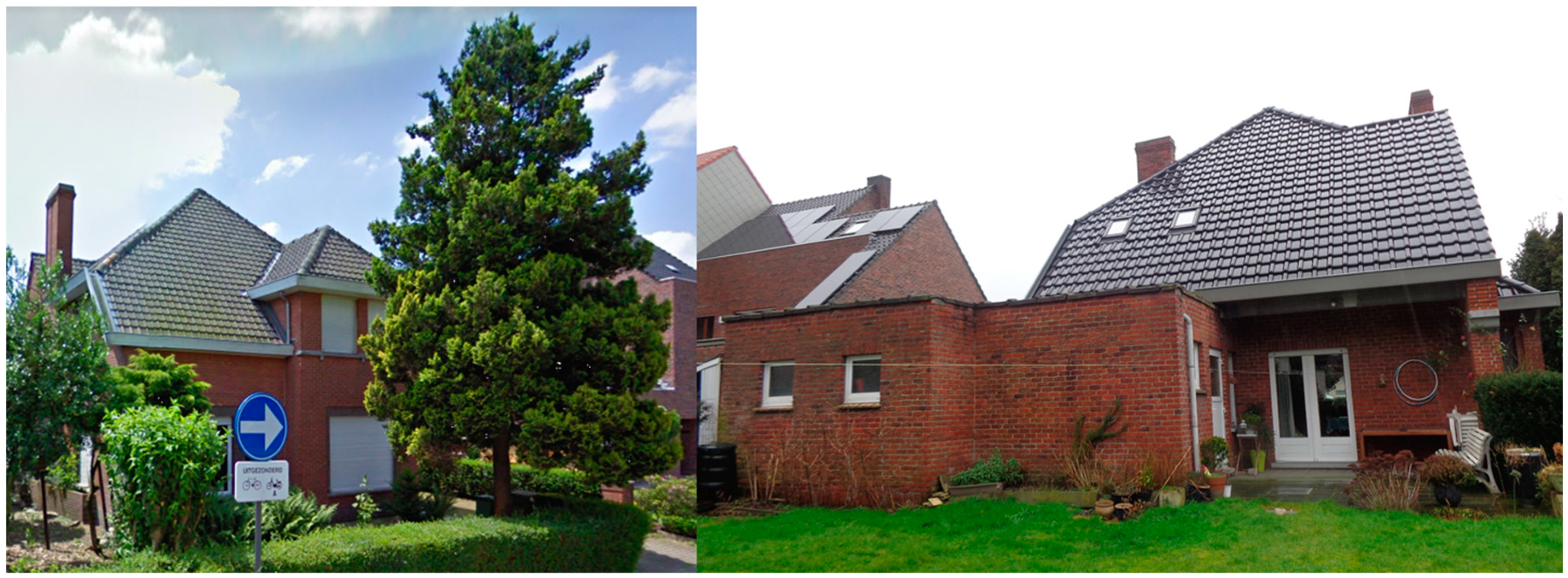
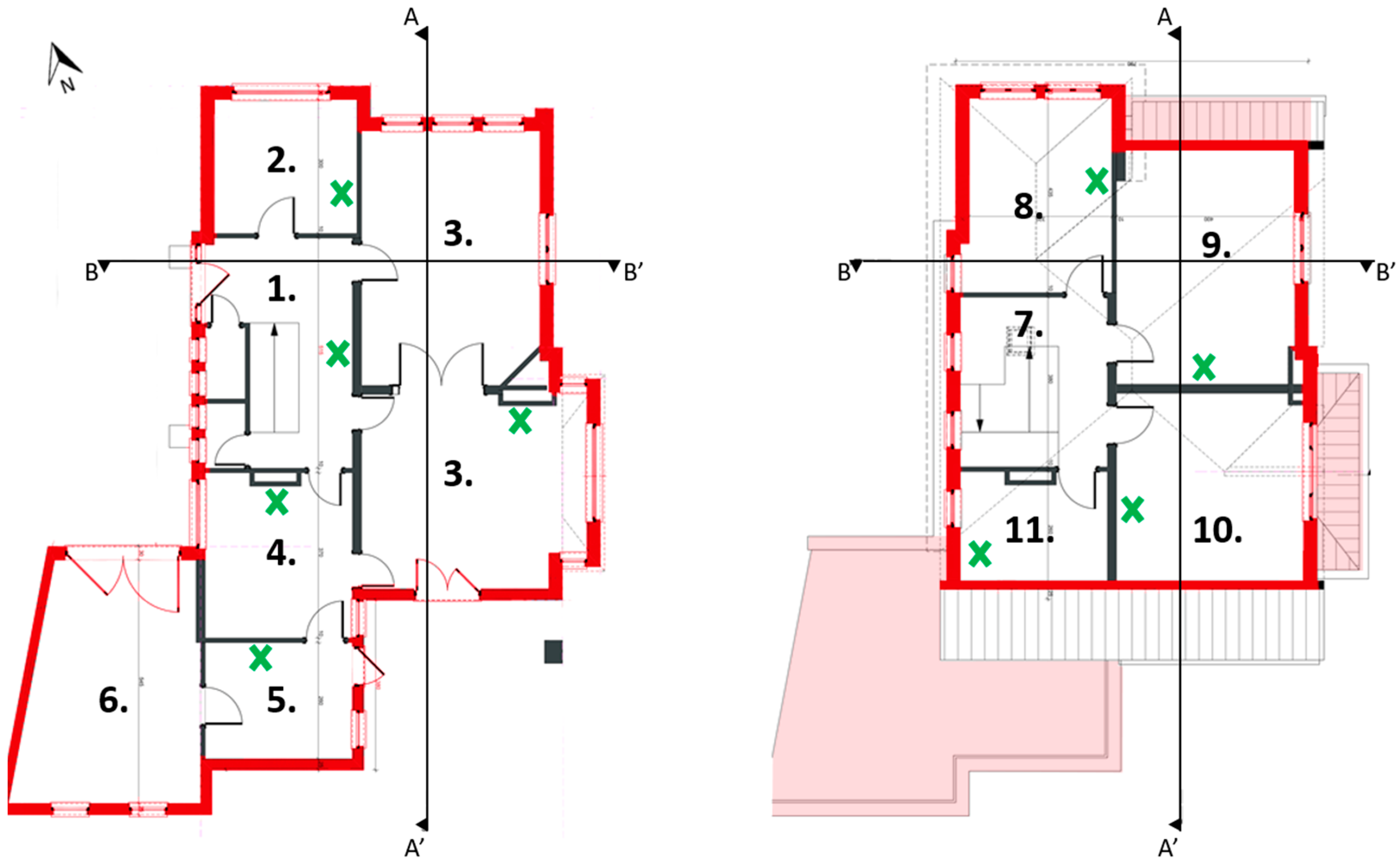
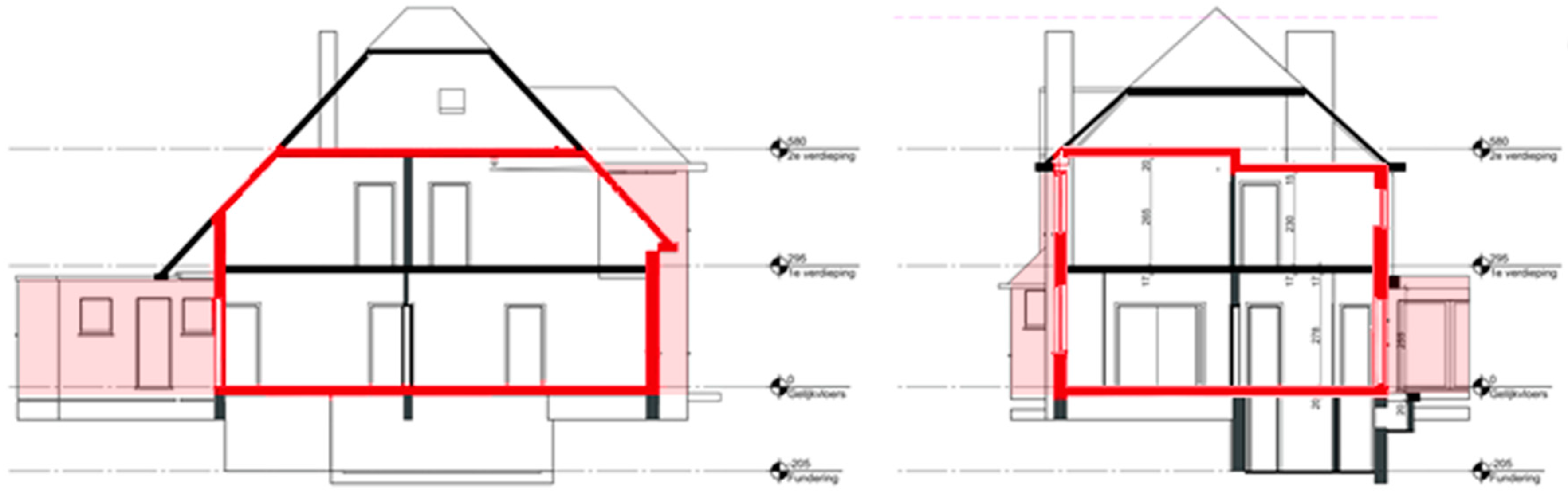
The following two sections subsequently describe the case study building, and the monitoring campaign to which it was subjected.

2.1. The Building

The case study building is a detached single family house in Ghent, Belgium. The dwelling has a gross floor area (measured externally, excluding the floor area of the attic and cellar) of 222.6 m², with 11 rooms spread over two floors. The ground floor includes a living room, a study, an entrance hall with a cloakroom and toilet, a kitchen, a utility room and a former garage that is used as an extra storage space. The first floor consists of a landing, three bedrooms, and a bathroom. In addition, the house has an attic space and a cellar underneath the entrance hall, cloakroom, and toilet. Elevations, floor plans of the ground and first floor, as well as cross sections can be found in Figure 1, Figure 2 and Figure 3.

The house is occupied by a family of two adults and one teenager, who are mostly absent between 8 a.m. and 5 p.m. on working days. Space heating is provided by a hydronic central heating system, with a gas-fired condensing boiler and radiators as heat emitters. The condensing boiler has a manufacturer’s quoted nominal power of 34.8 kW and a seasonal energy efficiency for space heating of 94% (against upper calorific value) [29], and is installed in the cellar. The control system adjusts the temperature of the boiler according to the outside temperature. No secondary heating systems are used. The interior temperature is controlled via a room thermostat in the living room and thermostatic radiator valves. Natural gas is furthermore used for cooking, and as primary source of energy for the production of domestic hot water (DHW). The condensing boiler in the cellar is not used to supply DHW. Instead, an electric boiler in the kitchen provides DHW for the kitchen sink, and a gas-fired boiler in the bathroom serves all other tapping points. Neither controlled ventilation nor active cooling are foreseen.

In a survey, the occupants indicated that only the radiators in the living room, kitchen, toilet, bathroom, and circulation area (entrance hall and landing) are actively used. However, it is assumed that the remainder of the rooms on the two floors (the bedrooms and storage rooms) are also considered as inhabited spaces and hence maintained at a reasonable temperature. This in contrast with the attic and cellar, which have no daily use. Therefore, this paper aims to assess the thermal performance of the building fabric separating the rooms on the ground and first floor from (1) the exterior environment, (2) the ground, and (3) the adjacent unconditioned spaces, namely the attic space and cellar. The building fabric of interest for the HLC characterization hence comprises the external walls, windows and doors, the slab-on-ground floor and floor above the cellar, the parts of the pitched roof above the bedrooms, the attic floor, and the flat roof. For clarity, these buildings components are marked in red in Figure 2 and Figure 3.

The dwelling was built in 1959, and its current owners have no knowledge of any alteration to the original construction of the external walls, floors, and flat roof. Hence, according to the national typology data base [30], the dwelling’s external brick walls can be assumed to include an uninsulated air cavity, and the slab-on-ground, and flat roof construction are most likely uninsulated. By contrast, the dwelling owners state that mineral wool was added to the original timber roof structure above the bedrooms, and 10 cm extruded polystyrene (XPS) was installed on top of the concrete attic floor. Based on this knowledge, the compositions listed in

Table 1. Composition, surface area (A), U-value, and temperature ratio (b_T) of the building components the building fabric of interest is composed of.

Building Component		Composition (From Inside to Outside, Layer Thicknesses in (m))	A (m2)	U (W/m2·K)	bT (-)
External wall	type 1	plaster finish (0.015), lightweight brick inner leaf (0.14), unfilled cavity (0.055), brick outer leaf (0.09)	133.1	1.3	1.0
	type 2	plaster finish (0.015), lightweight brick inner leaf (0.09), unfilled cavity (0.055), brick outer leaf (0.09)	55.4	1.5	1.0
	type 3	lightweight brick inner leaf (0.14), unfilled cavity (0.045), wood cladding (0.015)	16.5	1.4	1.0
Floor slab	on ground	tiles (0.01), sand bed (0.04), concrete slab (0.15)	111.8	0.9	1.0
	above cellar	tiles (0.01), sand bed (0.04), hollow-core concrete slab (0.15)	20.3	1.7	0.8
Attic floor	type 1	hollow-core concrete slab (0.15), XPS insulation (0.10)	38.1	0.3	0.9
	type 2	hollow-core concrete slab (0.20), XPS insulation (0.10)	33.8	0.3	0.9
Roof	pitched, type 1	gypsum board (0.014), rafters (0.15), oriented strand board (OSB) (0.02), battens and counter battens, ceramic tiles	22.8	1.6	1.0
	pitched, type 2	gypsum board (0.014), mineral wool with aluminum foil facing between rafters (0.15), oriented strand board (OSB) (0.02), battens and counter battens, ceramic tiles	15.0	0.4	1.0
	flat	gypsum board (0.014), wood frame layer (0.27), oriented strand board (OSB) (0.02), bitumen roofing	37.9	1.6	1.0
External doors		uninsulated polyvinyl chloride (PVC) door leaf	3.0	4.0	1.0
Garage door		uninsulated PVC door leaf	5.4	4.0	1.0
External Window	type 1	aluminum-framed double glazing with selective coating	22.7	1.8	1.0
	type 2	PVC-framed double glazing with selective coating	13.0	3.0	1.0
	skylight	PVC-framed double glazing with selective coating	1.5	1.6	1.0

are drawn up. These suggested compositions are consistent with the thicknesses of the building elements on the building plans, but could not be further confirmed.

In addition to the composition of the building components, Table 1 also summarizes their surface area and U-value. The former was measured on the building plans, the latter was calculated based on the default values for the thermal conductivity of material layers provided by the Flemish Energy Regulations for Buildings (EPB) [31]. With each of the building components, a temperature ratio b_T is associated, as expressed in Equations (3) and (4). For the elements in contact with the exterior this value equals 1. For those in contact with the unconditioned spaces, the constant default values suggested in the national addendum to the European standard EN 12831 [32] are used. These are 0.8 for the floor slab above the cellar and 0.9 for the attic floor (with the cellar categorized as ‘Basement with windows/external doors’ and the attic as ‘Roofspace, other non-insulated roof’). Finally, contrary to Equation (4), the b_T for the slab-on-ground is also set to 1, since its U-value is calculated to already incorporate the effect of the ground following the procedure described in ISO 13370 [33,34].

The dwelling has a window-to-wall ratio (WWR) of 14.8%. In 2012, 63.6% of the double glazed PVC windows (type 2, Table 1) were replaced by better performing aluminum-framed ones (type 1, Table 1). All windows, except those of the landing, have rolling shutters. These of the bedrooms are closed every night, these of the living room are closed at night during winter. The shutters are not accounted for in the U-values listed in Table 1.

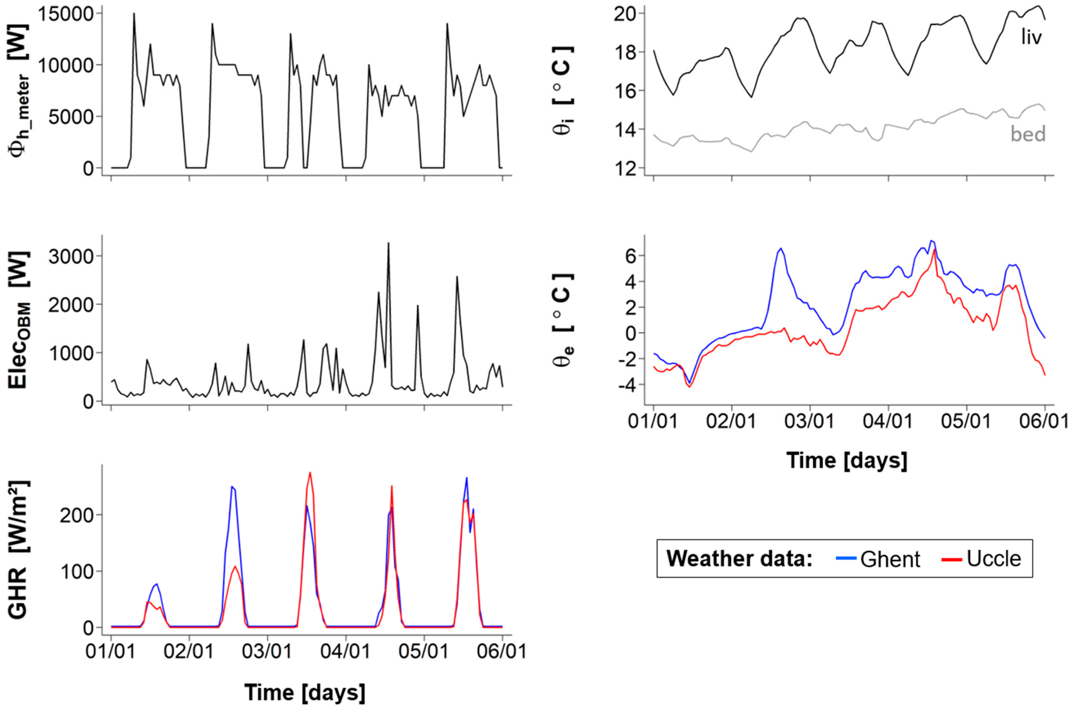
2.2. The Monitoring Campaign

The studied dwelling is a demonstration case of the ‘RenoseeC’ project [35], one of the 10 ‘Pilot Projects Renovation’ of the regional agency ‘Flanders Innovation & Entrepreneurship’ (Vlaio) [36]. In the framework of these projects dozens of dwellings across Flanders, with various typologies and resident profiles, have been subjected to a renovation with specific attention for energy efficiency measures. By carrying out measurements concerning the energy use and user comfort both before and after the retrofit, the research consortia aim to analyze the efficiency of the applied measures.

This paper assesses the energy performance of the case study dwelling before any energy saving measures were implemented in the framework of the RenoseeC project; the so-called ‘baseline performance’. Hence, the analyses consider the OBM data that was collected in a period stretching from November 11, 2016 to February 22, 2017. A description of the full data set is provided in

Table 2. Overview of the data collected during the on-board monitoring (OBM) campaign, as well as specifications of the instrumentation used.

Monitored Variable		Specifications of Instrumentation
Description	Abbreviation	type	Sampling time	Resolution	Accuracy
Heat output of the boiler for space heating	Φh,meter	Flow: Micronics, U1000 Temperature: JUMO, Pt500 Integrator: Zenner, multidata	10 min	1 kW·h	3% for flow, unspecified for temperature reading
Mains electricity consumption	ElecOBM	Fluksometer	5 min	1 W	2–6%
Interior temperature in the attic, cellar, and all rooms except for the former garage and landing.	θi,<room>	Onset, HOBO UX100-003	10 min	0.024 °C	0.21 °C
Exterior temperature (Ghent)	θe,Ghent	Vaisala, HMS82	1 min	0.00001 °C	0.3 °C
Global horizontal radiation (Ghent)	GHRGhent	Kipp&Zonen, SP Lite2	1 min	0.00001 W/m2	<10 W/m2
Exterior temperature (Uccle)	θe,Uccle	Thermibel, Pt100	1 h	0.1 °C	0.2 °C
Global horizontal radiation (Uccle)	GHRUccle	Kipp&Zonen, CNR1	1 h	0.1 W/m2	10%

. Figure 4 illustrates the collected monitoring data for five typical days at the beginning of January 2017.

The heat output of the condensing boiler for space heating was registered using a clamp-on heat meter. This device comprises (1) a flow meter, which was installed near the boiler outlet, (2) a pair of temperature sensors monitoring the inlet and outlet temperature, and (3) an integrator that calculates the actual heat output, which will be denoted as Φ_h,meter. Since the boiler and heat meter are installed in the cellar, some minor distribution losses could still occur outside the considered heated volume. Hence, Φ_h,meter does not fully equal Φ_h in Equations (5)–(7), but is presumed to closely approximate it. Given its cost, a heat meter is typically not available in dwellings. Alternatively, the natural gas consumption can be monitored using a smart meter. In that case, the gas consumption should be decomposed into its end uses (space heating, cooking, and DHW production) [37] and the system efficiency should be accounted for.

The mains electricity consumption drawn from the national grid was monitored as well (‘Elec_OBM’). Furthermore, the interior temperature θ_i was recorded in the attic space, the cellar, and all rooms on the ground and first floor, except for the former garage and the landing. The exact position of the sensors is indicated in the floor plans in Figure 2. Finally, monitoring data of the exterior air temperature θ_e and global horizontal radiation (GHR) were obtained from a local weather station in Ghent (geodesic distance of about 4 km to the case study dwelling).

In addition to the monitoring campaign, a blowerdoor test was performed to evaluate the airtightness of the building envelope. During the test, the doors to the cellar and attic were closed, all other doors on the ground and first floor remained open. Following the procedure described in NBN EN ISO 9972 [38], an n₅₀ value of 7.4/h was obtained.

For the sake of comparison, the OBM data set was supplemented with meteorological data (exterior temperature and global horizontal radiation) collected at a weather station of the Royal Meteorological Institute in Uccle (geodesic distance of about 51 km to the case study dwelling). In addition, historical annual data on the mains electricity and gas consumption was requested from the energy supplier.

3. Research Methodology

This paper aims to enhance the understanding of the impact of (1) the data analysis method and (2) the input data on the characterization outcome. The general principles of the evaluated data analysis methods are outlined in Section 3.1. Next, Section 3.2 delineates the different input data packages that are fed into the models. Finally, Section 3.3 gives more information on the approach that was adopted to fit and validate the models, and to determine the HLC estimate.

3.1. Data Analysis Methods

Four different data analysis methods will be applied to determine the HLC of the case study dwelling. The characterization capabilities of these methods have previously been compared based on synthetic monitoring data [39]. The methods considered are the Average method (‘Avg’), Linear Regression Analysis (‘LR’), the energy signature method (‘ES’), and ARX modeling (ARX stands for ‘AutoRegressive with eXogenous input’). The first three methods take the single-zone steady-state heat balance, which neglects the building’s actual dynamic behavior (Equation (12)), as a starting point. The ARX method, on the other hand, considers the building as a—still single-zone—dynamic system with energy that is being charged and discharged by the building’s effective thermal mass (Equations (5) and (6)).

Table 3. Overview of the model equations evaluated by the four data analysis methods. The Linear Regression Analysis (LR), energy signature method (ES), and AutoRegressive with eXogenous input (ARX) models consider vectors, as indicated by the notation in bold.

Method	Model Equation
Avg	$HLC={\displaystyle {\displaystyle \sum }_{j=1}^n}\left({\Phi }_{h;t_j}+{\Phi }_{int;t_j}+{\Phi }_{sol;t_j}+{\Phi }_{v;t_j}\right)/{\displaystyle {\displaystyle \sum }_{j=1}^n}\left({\theta }_{i;t_j}-{\theta }_{e;t_j}\right)$	(13)
LR	${\mathit{\Phi }}_{\mathit{h};\mathit{t}}+{\mathit{\Phi }}_{\mathit{i}\mathit{n}\mathit{t};\mathit{t}}+{\mathit{\Phi }}_{\mathit{s}\mathit{o}\mathit{l};\mathit{t}}+{\mathit{\Phi }}_{\mathit{v};\mathit{t}}=HLC·\left({\mathit{\theta }}_{\mathit{i};\mathit{t}}-{\mathit{\theta }}_{\mathit{e};\mathit{t}}\right)+{\mathit{\epsilon }}_{\mathit{t}}$	(14)
	${\mathit{\Phi }}_{\mathit{h};\mathit{t}}+{\mathit{\Phi }}_{\mathit{i}\mathit{n}\mathit{t};\mathit{t}}+{\mathit{\Phi }}_{\mathit{v};\mathit{t}}=HLC·\left({\mathit{\theta }}_{\mathit{i};\mathit{t}}-{\mathit{\theta }}_{\mathit{e};\mathit{t}}\right)+\left(-g{A}_l\right)·{\mathit{I}}_{\mathit{s}\mathit{o}\mathit{l};\mathit{k};\mathit{t}}+{\mathit{\epsilon }}_{\mathit{t}}$	(15)
ES	${\mathit{\Phi }}_{\mathit{i}\mathit{n}\mathit{t};\mathit{t}}+{\mathit{\Phi }}_{\mathit{s}\mathit{o}\mathit{l};\mathit{t}}+{\mathit{\Phi }}_{\mathit{v};\mathit{t}}=HLC·\left({\mathit{\theta }}_{\mathit{i};\mathit{t}}-{\theta }_b\right)+{\mathit{\epsilon }}_{\mathit{t}}$	(16)
	$\begin{array}{cc}{\mathit{\Phi }}_{\mathit{h};\mathit{t}}=& \{\begin{array}{cc}HLC·\left({\theta }_b-{\mathit{\theta }}_{\mathit{e};\mathit{t}}\right)+{\mathit{\epsilon }}_{\mathit{t}}\hfill & if{\mathit{\theta }}_{\mathit{e};\mathit{t}}<{\theta }_b\hfill \\ 0+{\mathit{\epsilon }}_{\mathit{t}}\hfill & if{\mathit{\theta }}_{\mathit{e};\mathit{t}}\ge {\theta }_b\hfill \end{array}\end{array}$	(17)
		(18)
ARX	$\phi \left(B\right)·\left({\mathit{\Phi }}_{\mathit{h};\mathit{t}}+{\mathit{\Phi }}_{\mathit{i}\mathit{n}\mathit{t};\mathit{t}}+{\mathit{\Phi }}_{\mathit{s}\mathit{o}\mathit{l};\mathit{t}}+{\mathit{\Phi }}_{\mathit{v};\mathit{t}}\right)={\omega }_i\left(B\right)·{\mathit{\theta }}_{\mathit{i};\mathit{t}}+{\omega }_e\left(B\right)·{\mathit{\theta }}_{\mathit{e};\mathit{t}}+{\mathit{\epsilon }}_{\mathit{t}}$	(19)
	$\phi \left(B\right)·{\mathit{\theta }}_{\mathit{i};\mathit{t}}={\omega }_h\left(B\right)·\left({\mathit{\Phi }}_{\mathit{h};\mathit{t}}+{\mathit{\Phi }}_{\mathit{i}\mathit{n}\mathit{t};\mathit{t}}+{\mathit{\Phi }}_{\mathit{s}\mathit{o}\mathit{l};\mathit{t}}+{\mathit{\Phi }}_{\mathit{v};\mathit{t}}\right)+{\omega }_e\left(B\right)·{\mathit{\theta }}_{\mathit{e};\mathit{t}}+{\mathit{\epsilon }}_{\mathit{t}}$	(20)
	$\phi \left(B\right)·{\mathit{\theta }}_{\mathit{i};\mathit{t}}={\omega }_h\left(B\right)·\left({\mathit{\Phi }}_{\mathit{h};\mathit{t}}+{\mathit{\Phi }}_{\mathit{i}\mathit{n}\mathit{t};\mathit{t}}+{\mathit{\Phi }}_{\mathit{v};\mathit{t}}\right)+{\omega }_e\left(B\right)·{\mathit{\theta }}_{\mathit{e};\mathit{t}}+{\omega }_{sol}\left(B\right)·{\mathit{I}}_{\mathit{s}\mathit{o}\mathit{l};\mathit{k};\mathit{t}}+{\mathit{\epsilon }}_{\mathit{t}}$	(21)

gives an overview of the model equations evaluated by the four methods.

$$C_i·d{\theta }_i/dt=0$$

(11)

$$\Downarrow$$

$${\mathit{\Phi }}_{\mathit{h};\mathit{t}}+{\mathit{\Phi }}_{\mathit{i}\mathit{n}\mathit{t};\mathit{t}}+{\mathit{\Phi }}_{\mathit{s}\mathit{o}\mathit{l};\mathit{t}}+{\mathit{\Phi }}_{\mathit{v};\mathit{t}}=-\left({\mathit{\Phi }}_{\mathit{i}\mathit{n}\mathit{f};\mathit{t}}+{\mathit{\Phi }}_{\mathit{t}\mathit{r};\mathit{t}}\right)=HL{C}_t·\left({\mathit{\theta }}_{\mathit{i};\mathit{t}}-{\mathit{\theta }}_{\mathit{e};\mathit{t}}\right)$$

(12)

The Average method, described in Equation (13), is a translation of the method proposed in ISO 9869-1 [40] to estimate the U-value of building components from on-site heat flux elements, to the building level. For each time step t_j at which an observation of the heat flow rates and temperatures is made, it determines (1) a total heat flow rate, which is the sum of the net heat input, internal and solar gains, and ventilation heat flow rate and (2) the difference between the interior and exterior temperature. It then divides the sum of the total heat flow rates for the n available observations by the summed temperature difference. This ratio is assumed to converge to the average HLC, if measurements are taken over a sufficiently long time.

The linear regression model expressed in Equation (14) uses the steady-state heat balance in Equation (12) as a simple linear regression equation of the form y = a · x + ε, with the temperature difference between the interior and exterior environment as sole independent variable (x) explaining the variance of the sum of the heat flow rates (y), and ε the prediction error. By fitting this model to the collected time series data, an HLC estimate is obtained as the coefficient of the independent variable, hence the slope of the regression line. Furthermore, Bauwens and Roels [41] and Senave et al. [39] demonstrated how, based on the definition of Φ_sol in Equation (9), a multiple linear regression equation can be drawn up (Equation (15)). This model can be used when monitoring data of the incident solar radiation under a certain projection (I_sol;k) is available instead of the solar gains. In addition to an HLC estimate, this model provides an estimate for a solar aperture coefficient or lumped gA-value (‘gA_l’). However, the authors [39] warn that the simplified representation of the solar gains in Equation (15), using a single projection of the solar radiation and a constant lumped gA-value, can lead to maximal deviations between the HLC estimate and actual HLC of more than 15%.

The Energy Signature method [42,43] is a special case of LR, which, beside the HLC, assesses a base temperature θ_b. This is the exterior temperature for which the building at temperature θ_i is in thermal balance with its environment and does not require space heating (Φ_h = 0) (Equations (16)–(18)). Notably, the equation from which the HLC can be derived, Equation (17), does not explicitly incorporate the interior temperature.

The ARX models [17,18,44] presented in Equations (19)–(21) are transfer function models aiming to describe the dwelling’s dynamic behavior. To this end, past observations (so-called ‘lags’) of the heat flow rates and temperatures are taken into account. Practically, this is done using output and input polynomials in the backshift operator B; respectively φ(B) (Equation (22)) and ω_x(B) (Equation (23)). The backshift operator hereby works as explained in Equation (24), with Z_t the observation of variable Z at time t. The numbers n_φ and n_ωx indicate the order of the polynomials. Two model variants will be applied, with the sum of the heat flow rates either as output (Equation (19)) or input (Equation (20)). Similar as for the LR model, a variant with I_sol as input variable will be considered, as demonstrated by Equation (21).

$$\phi \left(B\right)=1·B^0+{\phi }_1·B^1+{\phi }_2·B^2+\cdots +{\phi }_{n_{\phi }}·B^{n_{\phi }}$$

(22)

$${\omega }_x\left(B\right)={\omega }_{x,0}·B^0+{\omega }_{x,1}·B^1+\cdots +{\omega }_{x,n_{{\omega }_x}}·B^{n_{{\omega }_x}}$$

(23)

$$B^k·{\mathit{Z}}_{\mathit{t}}={\mathit{Z}}_{\mathit{t}-\mathit{k}}$$

(24)

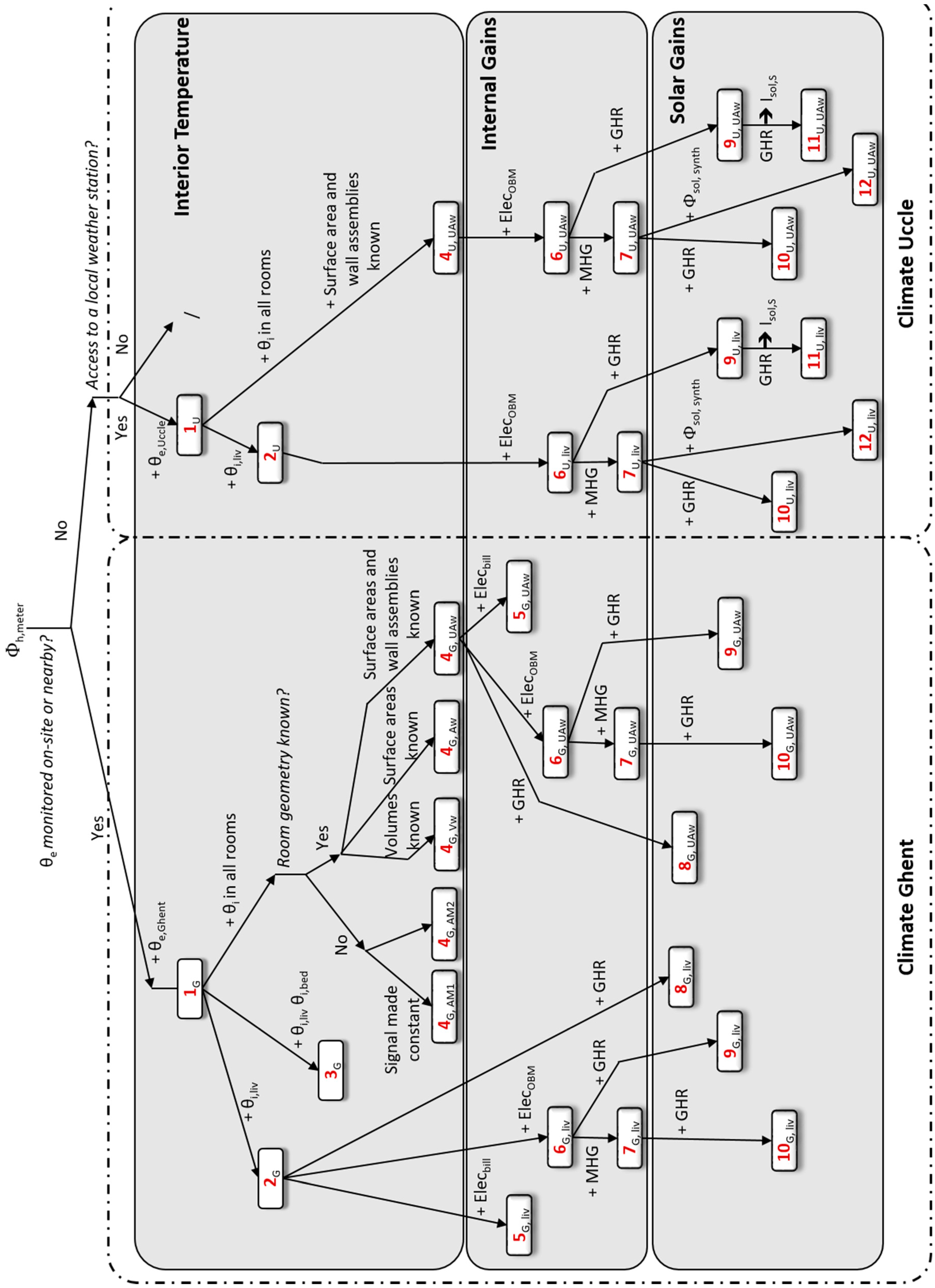
3.2. Input Data Packages

Table 3 shows that the analysis methods need input data for six variables: the heat flow rates Φ_h, Φ_sol, Φ_v, and Φ_int and the temperatures θ_i and θ_e. Acquiring all these data through on-board monitoring is, however, not always practically feasible and economically desirable. By following the procedure outlined in Figure 5 and

Table 4. Composition of the data packages, and the applied data analysis methods. The abbreviations ‘liv’, ‘bed’, ‘V’, and ‘MHG’ stand for, respectively, ‘living room’, ‘bedroom’, ‘volume’, and ‘metabolic heat gains’.

Data Package					Analysis Method
Name		Content			Avg.	LR	ES	ARX
		OBM Data	Additional Knowledge	Assumptions (*)
Impact of representation of exterior and interior temperature
1	1G	Φh,meter, θe,Ghent	/	θi = 18°C, Φint = 0, Φsol = 0	✓	✓	✓	✓
	1U	Φh,meter, θe,Uccle	/	θi = 18°C, Φint = 0, Φsol = 0,	✓	✓	✓	✓
2	2G	Φh,meter, θe,Ghent, θi,liv	/	θi = θi,living, Φint = 0, Φsol = 0	✓	✓		✓
	2U	Φh,meter, θe,Uccle, θi,liv	/	θi = θi,living, Φint = 0, Φsol = 0	✓	✓		✓
3G		Φh,meter, θe,Ghent, θi,liv, θi,bed	/	θi = θi,AM, Φint = 0, Φsol = 0	✓	✓		✓
4	4G,AM1	Φh,meter, θe,Ghent, θi all rooms	/	θi = mean(θi,AM), Φint = 0, Φsol = 0	✓	✓		✓
	4G,AM2	Φh,meter, θe,Ghent, θi all rooms	/	θi = θi,AM, Φint = 0, Φsol = 0	✓	✓		✓
	4G,Vw	Φh,meter, θe,Ghent, θi all rooms	Vrooms	θi = θi,Vw, Φint = 0, Φsol = 0	✓	✓		✓
	4G,Aw	Φh,meter, θe,Ghent, θi all rooms	Arooms	θi = θi,Aw, Φint = 0, Φsol = 0	✓	✓		✓
	4G,UAw	Φh,meter, θe,Ghent, θi all rooms	Arooms, U-values	θi = θi,UAw, Φint = 0, Φsol = 0	✓	✓		✓
	4U,UAw	Φh,meter, θe,Uccle, θi all rooms	Arooms, U-values	θi = θi,UAw, Φint = 0, Φsol = 0	✓	v		v
Impact of representation of internal heat gains
5	5G,liv	Φh,meter, θe,Ghent, θi,liv	electricity bill	θi = θi,living, Φint = Elecbill, Φsol = 0	✓	✓		✓
	5G,UAw	Φh,meter, θe,Ghent, θi all rooms	Arooms, U-values, electricity bill	θi = θi,UAw, Φint = Elecbill, Φsol = 0	✓	✓		✓
6	6G,liv	Φh,meter, θe,Ghent, θi,liv, ElecOBM	/	θi = θi,living, Φint = ElecOBM, Φsol = 0	✓	✓		✓
	6G,UAw	Φh,meter, θe,Ghent, θi all rooms, ElecOBM	Arooms, U-values	θi = θi,UAw, Φint = ElecOBM, Φsol = 0	✓	✓		✓
	6U,liv	Φh,meter, θe,Uccle, θi,liv, ElecOBM	/	θi = θi,living, Φnt = ElecOBM, Φsol = 0	✓	✓		✓
	6U,UAw	Φh,meter, θe,Uccle, θi all rooms, ElecOBM	Arooms, U-values	θi = θi,UAw, Φint = ElecOBM, Φsol = 0	✓	✓		✓
7	7G,liv	Φh,meter, θe,Ghent, θi,liv, ElecOBM	occupancy	θi = θi,living, Φint = (ElecOBM+MHG), Φsol = 0	✓	✓		✓
	7G,UAw	Φh,meter, θe,Ghent, θi all rooms, ElecOBM	Arooms, U-values, occupancy	θi = θi,UAw, Φint = (ElecOBM+MHG), Φsol = 0	✓	✓		✓
	7U,liv	Φh,meter, θe,Uccle, θi,liv, ElecOBM	occupancy	θi = θi,living, Φint = (ElecOBM+MHG), Φsol = 0	✓	✓		✓
	7U,UAw	Φh,meter, θe,Uccle, θi all rooms, ElecOBM	Arooms, U-values, occupancy	θi = θi,UAw, Φint = (ElecOBM+MHG), Φsol = 0	✓	✓		✓
Impact of representation of solar heat gains
8	8G,liv	Φh,meter, θe,Ghent, θi,liv, GHRGhent	/	θi = θi,living, Φint = 0, Φsol = gAl·GHRGhent (**)		✓		✓
	8G,UAw	Φh,meter, θe,Ghent, θi all rooms, GHRGhent	Arooms, U-values	θi = θi,UAw, Φint = 0, Φsol = gAl·GHRGhent (**)		✓		✓
9	9G,liv	Φh,meter, θe,Ghent, θi,liv, ElecOBM, GHRGhent	/	θi = θi,living, Φint = ElecOBM, Φsol = gAl·GHRGhent (**)		✓		✓
	9G,UAw	Φh,meter, θe,Ghent, θi all rooms, ElecOBM, GHRGhent	Arooms, U-values	θi = θi,UAw, Φint = ElecOBM, Φsol = gAl·GHRGhent (**)		✓		✓
	9U,liv	Φh,meter, θe,Uccle, θi,liv, ElecOBM, GHRUccle	/	θi = θi,living, Φint = ElecOBM, Φsol = gAl·GHRUccle (**)		✓		✓
	9U,UAw	Φh,meter, θe,Uccle, θi all rooms, ElecOBM, GHRUccle	Arooms, U-values	θi = θi,UAw, Φint = ElecOBM, Φsol = gAl·GHRUccle (**)		✓		✓
10	10G,liv	Φh,meter, θe,Ghent, θi,liv, ElecOBM, GHRGhent	occupancy	θi = θi,living, Φint = (ElecOBM+MHG), Φsol = gAl·GHRGhent (**)		✓		✓
	10G,UAw	Φh,meter, θe,Ghent, θi all rooms, ElecOBM, GHRGhent	Arooms, U-values, occupancy	θi = θi,UAw, Φint = (ElecOBM+MHG), Φsol = gAl·GHRGhent (**)		✓		✓
	10U,liv	Φh,meter, θe,Uccle, θi,liv, ElecOBM, GHRUccle	occupancy	θi = θi,living, Φint = (ElecOBM+MHG), Φsol = gAl·GHRUccle (**)		✓		✓
	10U,UAw	Φh,meter, θe,Uccle, θi all rooms, ElecOBM, GHRUccle	Arooms, U-values, occupancy	θi = θi,UAw, Φint = (ElecOBM+MHG), Φsol = gAl·GHRUccle (**)		✓		✓
11	11U,liv	Φh,meter, θe,Uccle, θi,liv, ElecOBM, GHRUccle	solar radiation algorithm	θi = θi,living, Φint = ElecOBM, Φsol = gAl·Isol,S,Uccle (**)		✓		✓
	11U,UAw	Φh,meter, θe,Uccle, θi all rooms, ElecOBM, GHRUccle	Arooms, U-values, solar radiation algorithm	θi = θi,UAw, Φint = ElecOBM, Φsol = gAl·Isol,S,Uccle (**)		✓		✓
12	12U,liv	Φh,meter, θe,Uccle, θi,liv, ElecOBM, GHRUccle	occupancy, window positioning, solar radiation algorithm	θi = θi,living, Φint = (ElecOBM+MHG), Φsol = Φsol,synth	✓	✓		✓
	12U,UAw	Φh,meter, θe,Uccle, θi all rooms, ElecOBM, GHRUccle	Arooms, U-values, occupancy, window positioning, solar radiation algorithm	θi = θi,UAw, Φint = (ElecOBM+MHG), Φsol = Φsol,synth	✓	✓		✓

(*) in addition to the basic assumptions that the measured exterior temperature and the measurements of the heat meter (Φ_h,meter) can be used to represent θ_e and Φ_h, respectively. Since no intended ventilation is foreseen, Φ_v is furthermore set to zero. (**) with gA_l to be fitted.

it will therefore be analyzed what the impact is of neglecting these variables or using several alternative data sources to represent them.

The study follows the framework depicted in the tree structure of Figure 5. Each of the nodes of this tree represents a ‘data package’. These packages draw from two different data sources: ‘OBM’ (e.g., temperatures and energy consumption data) and ‘additional knowledge’ (e.g., building plans and occupant surveys). To ensure that an input value is available for each of the six variables mentioned above, these two types of data sources are further supplemented with some ‘assumptions’ (e.g., default values). Table 4 details the content of all 35 data packages. The different packages are visualized as the nodes of a tree-diagram in Figure 5, because they are nested, in the sense they are hierarchically extending one another with more information along the branches of the tree. The leaf nodes hence represent the richest data packages. This is also reflected in the naming of the packages. Each data package is denoted with a number and one or more letters. In general, the higher the package number, the more ‘OBM data’ or ‘additional knowledge’ the package embeds. Packages with the same number (depicted on the same level in Figure 5) aim to compare either the effect of alternative representations of a certain variable (e.g., packages 4) or the influence of the ancestor package to which a certain data source is added (e.g., packages 6). The letters help to distinguish between these packages of the same generation.

The exploration of the branches is structured around three topics: ‘Interior temperature’, ‘Internal heat gains’ and ‘Solar heat gains’. In addition, the influence of the spatial variability of the climate data on the HLC outcome will be assessed throughout the whole analysis.

The monitoring data collected by the heat meter, Φ_h,meter, is presumed to be essential for the HLC characterization and forms the root of the tree. In subsequent steps, data is added, resulting in 35 data packages.

Packages 1: By supplementing Φ_h,meter with exterior temperature data, collected at a nearby weather station in Ghent, a first data package is created; ‘1_G’ (see Figure 5). This package considers Φ_h,meter and θ_e,Ghent to respectively represent Φ_h and θ_e in the analysis methods (Table 3). In the absence of data on the actual interior temperature, a constant profile of 18 °C is assumed, in accordance with the Flemish Energy Regulations for Buildings (EPB) [45]. As a first, conservative guess, the unknown variables Φ_sol and Φ_int are set to zero (see Table 4). A second package, 1_U, starts from the same assumptions, but uses the more remotely registered exterior temperature data (θ_e,Uccle instead of θ_e,Ghent).

Packages 2 to 4: In a next step, the impact of adding interior temperature sensors to the OBM setup is analyzed through packages 2, 3, and 4. These packages respectively comprise one interior temperature sensor (in the living room), two sensors (in the living room and master bedroom, which is room No. 9 in Figure 2), and nine sensors spread over the dwelling. When multiple interior temperature signals are available, the question arises how they should be combined to approximate the equivalent homogenous dwelling temperature θ_i. The sibling packages 4_G therefore examine how the characterization outcome differs when θ_i is represented by

• the arithmetic mean of all available interior temperature signals θ_i,AM (packages 4_G,AM1 with θ_i = mean(θ_i,AM) and 4_G,AM2 with θ_i = θ_i,AM);
• their (gross) room volume weighted average θ_i,Vw (package 4_G,Vw);
• their heat loss area weighted average θ_i,Aw (package 4_G,Aw);
• their UA-value weighted average θ_i,UAw (package 4_G,UAw);

In the case of the latter two the temperature ratios b_T are also taken into account, as shown in Equations (25) and (26) with j the rooms where the temperature was monitored (see Figure 2) and k the building components separating these room interiors from the ground, cellar, attic, or exterior environment. In reality these ratios are time dependent (see further, Section 4.2), but for the calculations in Equations (25) and (26) the constant values listed in Table 1 are used.

$${\theta }_{i,Aw;t}={\displaystyle \sum }_j\left({\displaystyle \sum }_k\left(A_{j,k}·b_{T;j,k}\right)·{\theta }_{i;j;t}\right)/{\displaystyle \sum }_j\left({\displaystyle \sum }_k\left(A_{j,k}·b_{T;j,k}\right)\right)$$

(25)

$${\theta }_{i,UAw;t}={\displaystyle \sum }_j\left({\displaystyle \sum }_k\left(U_{j,k}·A_{j,k}·b_{T;j,k}\right)·{\theta }_{i;j;t}\right)/{\displaystyle \sum }_j\left({\displaystyle \sum }_k\left(U_{j,k}·A_{j,k}·b_{T;j,k}\right)\right)$$

(26)

These approaches assume the room air to be perfectly mixed. Moreover, since the sensors were not installed in every room, the measurements collected in the utility room (No. 5 in Figure 2) are considered to be representative for both this room and the former garage (No. 6), especially since the occupants state that the connecting door is rarely closed. Similarly, the interior temperature registered in the entrance hall (No. 1 in Figure 2) is equally used for the cloakroom, toilet, and landing (No. 7).

Packages 5 to 7: Internal heat gains are caused by the presence of occupants and the use of appliances, lighting, hot water, and HVAC systems (Equation (8)). Setting Φ_int equal to zero might therefore be a too conservative assumption. To get insight into the sensitivity of the HLC outcome to the value used to represent Φ_int, packages 5 to 7 evaluate three options. First, packages 5 and 6 focus on the appliances induced internal heat gains (Φ_int = Φ_int,Ap&Li) and approximate these based on two different data sources. Packages 5, on the one hand, include historical electricity consumption data inquired from the energy provider. The cumulative electricity use was available for three different periods. Since the first period (September 1, 2012 till April 23, 2013; this is 234 days) mainly corresponds to the winter period considered here, an hourly averaged value Elec_bill (W) is determined as (cumulative electricity use period 1 (Wh))/(234·24h). This constant value will be used to represent Φ_int in packages 5_G. Packages 6, on the other hand, comprise the OBM mains electricity consumption data Elec_OBM to approximate Φ_int. Hence, in both cases, all electricity consumed by appliances and lighting is considered to be converted into heat and form a useful contribution to the dwelling’s interior temperature.

Subsequently, package 7 adds an approximation of the metabolic heat gains (MHG) (Φ_int,Occ in Equation (8)) to the Φ_int-value of package 6. This way it aims to obtain an HLC value that is less influenced by occupant presence and behavior. Based on a survey, the occupancy profile shown in the first two rows of

Table 5. Proposed occupancy and metabolic heat gain (MHG) profile. M and F stand for male and female.

Time Period	11 p.m.–7 a.m.	7 a.m.–9 a.m.	9 a.m.–5 p.m.	5 p.m.–8 p.m.	8 p.m.–11 p.m.
Number of persons, M/F	1 M, 2 F	1 M, 2 F	0	1 M, 2 F	1 M, 2 F
Activity	sleeping	standing, medium activity	-	standing, medium activity	sedentary activity
MHG (W)	200	575	0	575	350

is proposed. In combination with the default metabolic heat rates prescribed by ISO 8996 [46], and assuming a body surface area of 1.8 m² for men and 1.6 m² for women [46], this leads to the MHG-profile in the third row of the table. This daily profile will be repeated throughout the training and validation period of the analysis models.

Packages 8 to 12: By adding GHR data, registered in a weather station in either Ghent or Uccle, to the packages 2 (or 4), 6 and 7, the packages 8, 9, and 10 are created. This additional variable allows to replace the zero assumption for Φ_sol by (gA_l·GHR) and thus use model Equations (15) and (21) instead of Equations (14) and (20) to fit the LR and ARX models. In this context, packages 11 furthermore examine the change observed when the incident radiation on a vertical, south oriented surface (I_sol,S) is used instead of the GHR, the south orientation being selected because of its dominance in the northern hemisphere. I_sol,S is here inferred from the GHR data with the aid of the building energy simulation tool TRNSYS 17 [47], and in particular Type 99 [48]. Finally, packages 12 presume the positioning and geometry of the windows to be known. In combination with the GHR data, this allows to synthetically approximate the actual solar gains (Φ_sol,synth). Again, this task is performed using TRNSYS 17. Due to missing observations and small anomalies in the GHR data collected in Ghent, it was not possible to calculate I_sol,S or Φ_sol,synth for this climate. Hence, packages 11 and 12 were only developed for the weather data of Uccle.

The right part of Table 4 indicates which data analysis methods are applied on the different packages. The Average method (Equation (13)) can solely be used when an estimate for Φ_sol is available, not when it is fitted based on the GHR or I_sol,S data as is done in packages 8–11. Linear regression and ARX models are identified on all packages. In the majority of cases, this concerns the expressions given in Equation (14) and Equation (20). However, when data on the GHR or I_sol,S is available, Equation (15) and Equation (21) are applied instead. For package 1, where θ_i is considered to be constant, a version of the ARX model described in Equation (19), with Φ_h as output and θ_i as a constant, also needs to be used instead of Equation (20). The ES method is exclusively applied on the first package, since this is the only scenario where no measurement data is available to represent θ_i.

3.3. Model Fitting and Validation, Determination of HLC

Data analysis was performed in R [49]. The full data set spans over 104 days, from November 10, 2016 till February 22, 2017. The first 90 days (until February 8, 2017) were used to train all models, while the two last weeks were used as a cross-validation period for the ARX models.

To fulfill the steady-state requirements of the Average, Energy Signature, and Linear Regression method, the original monitoring data was resampled to a multiple of 12 h before using it as input. The exact resampling times were determined by two model validation criteria:

(a)

All model coefficients should prove to be significantly different from zero in a marginal t-test (p-value < 0.05).

(b)

The residuals of the fitted model should resemble white noise, which is a sequence of uncorrelated zero mean random variables [18]. This property is examined in both the time and frequency domain, by inspecting the plots of the Autocorrelation Function (‘ACF’) and the cumulated periodogram (‘CP’), respectively. In the former plot, it is verified whether the conditions specified in the IEA Annex 58 statistical guidelines [44] are fulfilled. These state that not more than 5–10% of the lag correlations should be significantly different from zero (exceed above the 95% confidence bands). Especially the correlation for the shorter lags and the 24 h lag should be insignificant. The CP, on the other hand, should approximate a linearly increasing function, indicating that the residuals do not have excess of a certain frequency. Its plot should thus show a quasi-straight line, that barely (5%) exceeds the 95% confidence band.

For 23 out of the 35 data packages listed in Table 4, 24 h proved to be the lowest resampling time (RST) for which the above criteria were met for the steady-state models. For the other 12 packages, the steady-state models were not valid for an RST of 12 h or any multiple of 12 h up to and including 120 h, as will be discussed in Section 4.

For the dynamic ARX models, six-hourly input data are used. The model order is determined using a forward modeling procedure:

• The model parametrization expressed in Equation (19), (20), or (21) is fitted to the data, allowing one lag for the autoregressive variable and 0 lags for the input variables (n_φ = 1, n_ωx = 0).
• The insignificant model coefficients are systematically removed, starting with those of the highest order present. After each elimination, the model is refitted. This step is repeated until only significant model coefficients remain.
• If the model passes the white noise criterion specified in (b), it is accepted. Otherwise, another lag is added to each variable (lag x for the input polynomials and lag (x + 1) for the output polynomial, whereby lag x is the next lag that has not been added before: the same lag is never added again if it was eliminated before), increasing the model order, and step 2 is repeated.

To test the ARX models for overfitting, the models are challenged to predict the interior temperature (or Φ_h in case of package 1) for 2 weeks in both the training and validation period, using one-step ahead prediction [26]. The normalized RMSE (nRMSE (%)) [26] between the predicted and measured interior temperature is then compared for both periods to verify if they are of the same order of magnitude. In this case, the maximum difference between the nRMSEs proves to be 32.7%, which was considered to be acceptable.

The HLC estimate of the Avg method follows from the ratio in Equation (13), and the method provides no confidence band [39]. To obtain the estimates for the LR and ES method, Equations (14), (15) and (17) are identified on the data set via the R-function ‘linear model’ (‘lm’), which applies ordinary least squares (OLS) regression [50]. This function returns both the mean estimate and standard deviation of all fitted model coefficients. In the case of the LR models, the coefficient of the temperature difference term represents the HLC, for the ES model, this is the coefficient of θ_e. Finally, for the ARX models, the HLC estimate needs to be derived from the steady-state gains using Lagrange weighting, as shown in Equation (27) for model Equation (19) and Equation (28) for model Equations (20) and (21) [26,39,44,51]. The steady-state gains of the variables are their polynomials with the backshift operator B set equal to 1 (e.g., ω_e(1)). This way, they represent the model’s steady-state behavior. The lambda in Equations (27) and (28) is the Lagrange multiplier, which ensures that the steady-state gain ratio with the highest variance (either H_i or H_e) gets the lowest weight when the HLC is inferred. To this end, λ considers the variance (‘Var’) and covariance (‘Cov’) of both (Equation (29)). For ARX models where θ_i is set to be a constant, no value is obtained for H_i and HLC is taken equal to H_e. To assess the uncertainty of the HLC estimates from ARX modeling, 50,000 random realizations are simulated of the fitted polynomials. From the resulting HLC values, a 95% confidence interval is derived. This procedure is also known as bootstrapping [52].

$$\left(\frac{{\omega }_i\left(1\right)}{\phi \left(1\right)}=H_i\right) \& \left(\frac{{\omega }_e\left(1\right)}{\phi \left(1\right)}=H_e\right) \to HLC=\lambda ·H_i+\left(1-\lambda \right)·H_e$$

(27)

$$\left(\frac{\phi \left(1\right)}{{\omega }_h\left(1\right)} =H_i\right) \& \left(\frac{{\omega }_e\left(1\right)}{{\omega }_h\left(1\right)}=H_e\right) \to HLC=\lambda ·H_i+\left(1-\lambda \right)·H_e$$

(28)

$$\lambda =\frac{Var\left(H_e\right)-Cov\left(H_i,H_e\right)}{Var\left(H_i\right)+Var\left(H_e\right)-2·Cov\left(H_i,H_e\right)}$$

(29)

4. Results and Discussion

This fourth section presents and discusses the main research findings. First, Section 4.1 shows the results of the HLC characterization based on OBM data and the sensitivity analysis. Thereafter, Section 4.2 compares the outcome of the OBM characterization with the theoretical HLC value calculated according to the governing standards.

4.1. Sensitivity Analysis

The discussion on the sensitivity of the HLC estimate will be organized around the three topics indicated in Figure 5: the impact of the way (1) the interior temperature is represented, (2) the internal heat gains are approximated, and (3) the solar heat gains are modeled.

Based on the steady-state heat balance (Equation (12), rewritten in Equation (30)), it is expected that an underestimation of the dwelling’s equivalent homogenous temperature θ_i results in an overestimation of the transmission and infiltration losses per degree Kelvin temperature difference, and hence an overestimation of the HLC. Neglecting the internal or solar heat gains, and thus underestimating the real heat flow into the zone, on the other hand, is expected to lead to an underestimation of the HLC.

$$HL{C}_t=\frac{\left({\Phi }_{h;t}+{\Phi }_{int;t}+{\Phi }_{sol;t}+{\Phi }_{v;t}\right)}{\left({\theta }_{i;t}-{\theta }_{e;t}\right)}=\frac{-\left({\Phi }_{inf;t}+{\Phi }_{tr;t}\right)}{\left({\theta }_{i;t}-{\theta }_{e;t}\right)}$$

(30)

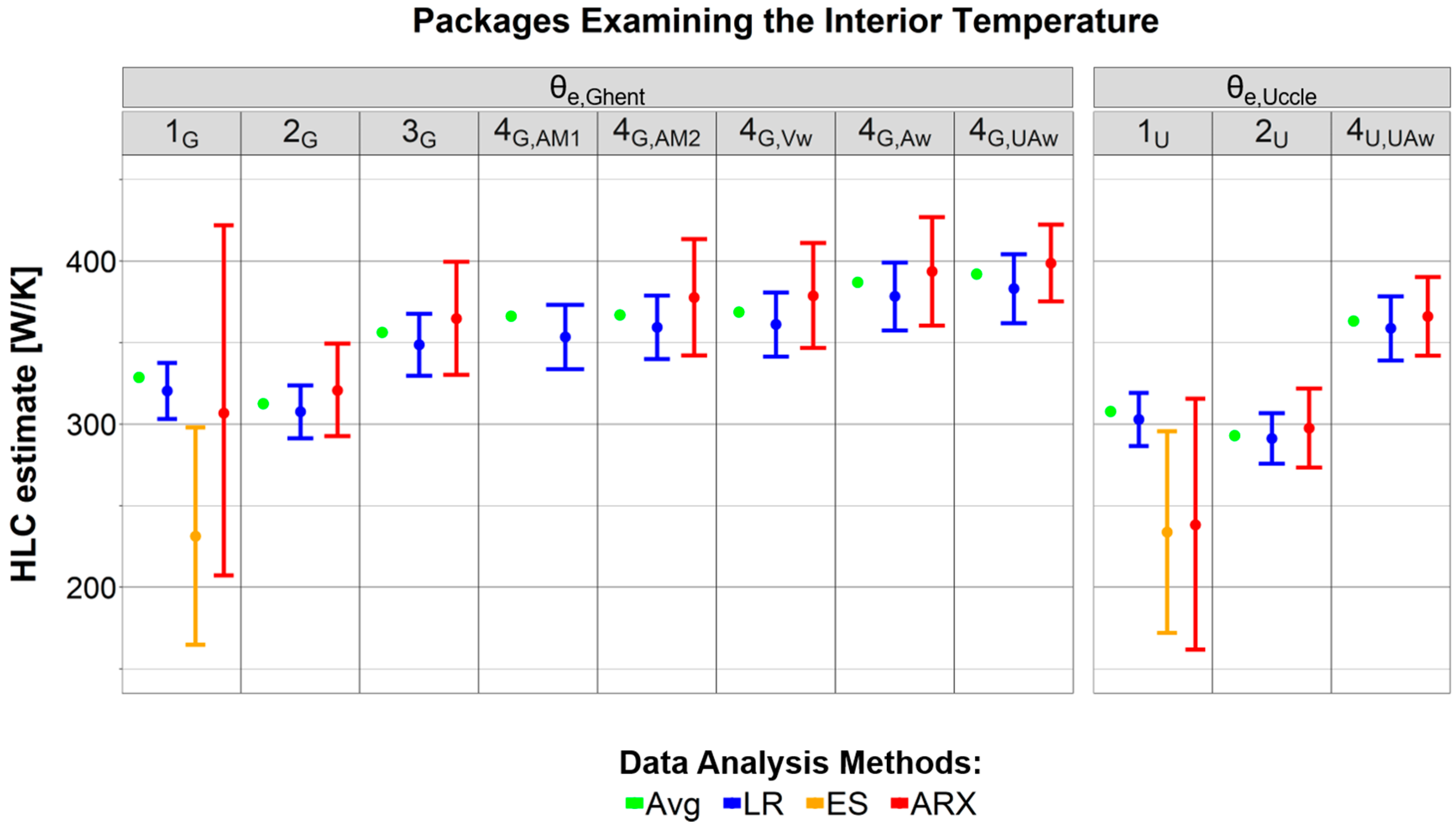
4.1.1. Impact of Representation of Exterior and Interior Temperature

Figure 6 gives an overview of the HLC estimates that are identified by the Average method, Linear Regression, Energy Signature method, and ARX models on the first four groups of data packages (see Table 4 and Figure 5). The left side of the figure investigates the sensitivity of the characterization outcome to the number of interior sensors installed, using the exterior temperature data collected in Ghent (θ_e,Ghent). The right side of the figure repeats some of the key analyses, using θ_e,Uccle instead of θ_e,Ghent.

Using a Default Value for the Interior Temperature

For data package 1_G, the Average and Linear Regression method return fairly consistent estimates of respectively 328.7 and 320.4 W/K. The 95% confidence interval (CI) associated with the LR estimate moreover has a range of 34.4 W/K, and thus includes the Avg estimate. The Energy Signature (ES) method is the only method that does not require an input for θ_i. It can be seen that this model structure results in a relatively low estimate of 231.4 W/K with a 95% CI that includes neither the Avg nor the LR estimate. The ES model hereby assumes a rather high base temperature θ_b of 23.5 °C. These findings are in line with those of the theoretical exercise in [39], where the accuracy of the ES method was also questioned. The HLC estimate of the ARX model is also lower than those of the Avg and LR methods. However, what is particularly striking is the estimate’s large 95% CI (range of 214.6 W/K). Senave et al. [26] analyzed the capability of ARX models for HLC characterization, using synthetic OBM data generated via simplified simulation models. They showed that, when transmission heat losses to the ground are not explicitly modeled, as is the case here, setting the intercept term in the ARX model structure equal to zero gives more precise and accurate HLC estimates. As an explanation, the authors have suggested that forcing the model structure through zero might help to avoid that part of the constant physical phenomena are wrongly attributed to a non-zero intercept. The assumption of a constant indoor temperature θ_i equal to 18 °C in data package 1 in this paper causes the ARX model to include a constant term, which might similarly lead to a more uncertain HLC estimate.

Installing One or More Interior Temperature Sensors

Comparing the results for data packages 1_G and 2_G in Figure 6, it seems that the living room temperature in this case rather closely corresponds to the default value of 18 °C. The HLC estimates for the second package deviate only 4.0% to 4.9% from those of package 1_G, depending on the applied analysis method.

Table 6. Mean and standard deviation (Sd) of the interior temperature signals tested in packages 2–4 over the training period. Figures are based on the six-hourly values that are used as input for the ARX models.

Temperature Signal	θi,liv	θi,AM(bed, liv)	θi,AM(all) = θi,AM2	θi,Vw	θi,Aw	θi,UAw	θe,Ghent	θe,Uccle
Mean (°C)	18.7	17.0	16.6	16.6	16.0	15.9	4.47	3.94
Sd (°C)	1.00	0.93	1.13	1.07	1.14	1.16	3.70	4.03

indeed confirms this: the mean value of θ_i,liv over the training period is 18.7 °C. It can furthermore be noted that the use of a varying interior temperature signal in 2_G yields quite consistent results for the three analysis methods, with the largest deviation between the mean estimates being 4.2% (Figure 6). The dynamic model exhibits the largest uncertainty, with the range of the 95% CI equaling 56.7 W/K. This is, however, significantly lower than the 95% CI associated with the ARX estimate for case 1_G.

However, more than one interior temperature sensor might be required to establish a reasonable estimate for the overall dwelling temperature, as demonstrated by the HLC estimates for packages 3_G and 4_G. Still, the exact number of temperature sensors that is needed will largely depend on the set-point temperature profiles that are applied in the different rooms, the thermal resistance of the building envelope and internal partitions, and the representativeness of the places where the temperature sensors are installed. In this specific case, the biggest change in HLC estimates is observed when a sensor is added in the master bedroom from package 2_G towards 3_G. Compared to the living room, this is a room that is not actively heated. Taking the arithmetic mean of the measurements of both sensors hence results in a relative reduction of the input signal used for θ_i, and as a consequence, the HLC estimate increases by 13.3% to 14.0%, depending on the applied data analysis method. The combination of these two sensors on the two floors proves to already yield a quite representative approximation for the mean dwelling temperature. The installation of seven extra sensors compared to package 3_G only alters the HLC estimate by 3.0% to 3.5%, when the arithmetic mean of the interior temperature signals is considered (θ_i,AM2, package 4_G,AM2). The fact whether a constant (4_G,AM1) or variable (4_G,AM2) mean signal is used, does not seem to significantly affect the HLC estimate. Notably, the ARX model is not applied on 4_G,AM1, since this would return the same result as for package 1_G.

For this dwelling geometry, the volume weighted interior temperature θ_i,Vw nearly equals the arithmetic mean θ_i,AM2: their mean values for the training period both amount to 16.6 °C (see Table 6), and the RMSE between the signals is 0.2 °C. As a result, the HLC estimates of 4_G,AM2 and 4_G,Vw are almost identical. By contrast, using prior knowledge on the surface area A and temperature ratios b_T of the building components to weight the interior temperature signals leads to a raise of the HLC estimates by 4.2–5.5%, compared to estimates based on the arithmetic mean temperature (package 4_G,Aw vs. 4_G,AM2). These numbers further increase to 5.6–6.8% when the U-values are used as well to weight the different room temperatures. In total, the HLC outcome even increases with about 1/4th when using θ_i,UAw instead of θ_i,liv for the characterization. This raise of the HLC can be linked to the use of a lower input signal for θ_i. The temperature measured in the utility room, which is on average the lowest throughout the model training period, gets the highest weight (29.6%) in θ_i,UAw. As a consequence, this weighted signal is on average up to 2.8 °C lower than that of θ_i,liv (see Table 6). Physically, combining the room temperatures based on the transmission heat transfer rates of their enclosing walls, seems the most sensible approach. It should however be noted that the airtightness of the building components—the other aspect of the HLC—is not taken into account in θ_i,UAw. Additionally, the uncertainty on the actual UA-values propagates further in the weighted temperature.

Using a Different Exterior Temperature Signal

The six-hourly averaged exterior temperature signal measured in Uccle has as a slightly lower mean (3.9 °C compared to 4.5 °C) and higher variance (16.2 °C² compared to 13.7 °C²) than the one measured in Ghent. The RMSE between θ_e,Uccle and θ_e,Ghent is 1.2 °C. As can be observed on the right side of Figure 6, using θ_e,Uccle for the characterization yields almost the same differences among the HLC estimates for the various representations of θ_i. The Avg and LR results based on the living room temperature (package 2_U) are respectively 4.8% and 3.8% lower than when a constant interior temperature of 18 °C is assumed (package 1_U). The relative increase between the results for packages 2_U and 4_U,UAw also amounts to 23.1–24.0%, depending on the applied analysis method. However, in absolute numbers, the estimates based on θ_e,Uccle are 5.3–7.2% lower than those based on θ_e,Ghent for package 2. This difference between both versions increases with an additional percent for packages 4_UAw. The deviations observed between the HLC estimates for both exterior temperature signals roughly correspond to the ones observed between the temperature differences used as model input. The differences between the interior and exterior temperature signal considered in packages 2_U and 4_U,UAw are on average, respectively, 4% and 5.2% higher than the temperature differences considered in packages 2_G and 4_G,UAw.

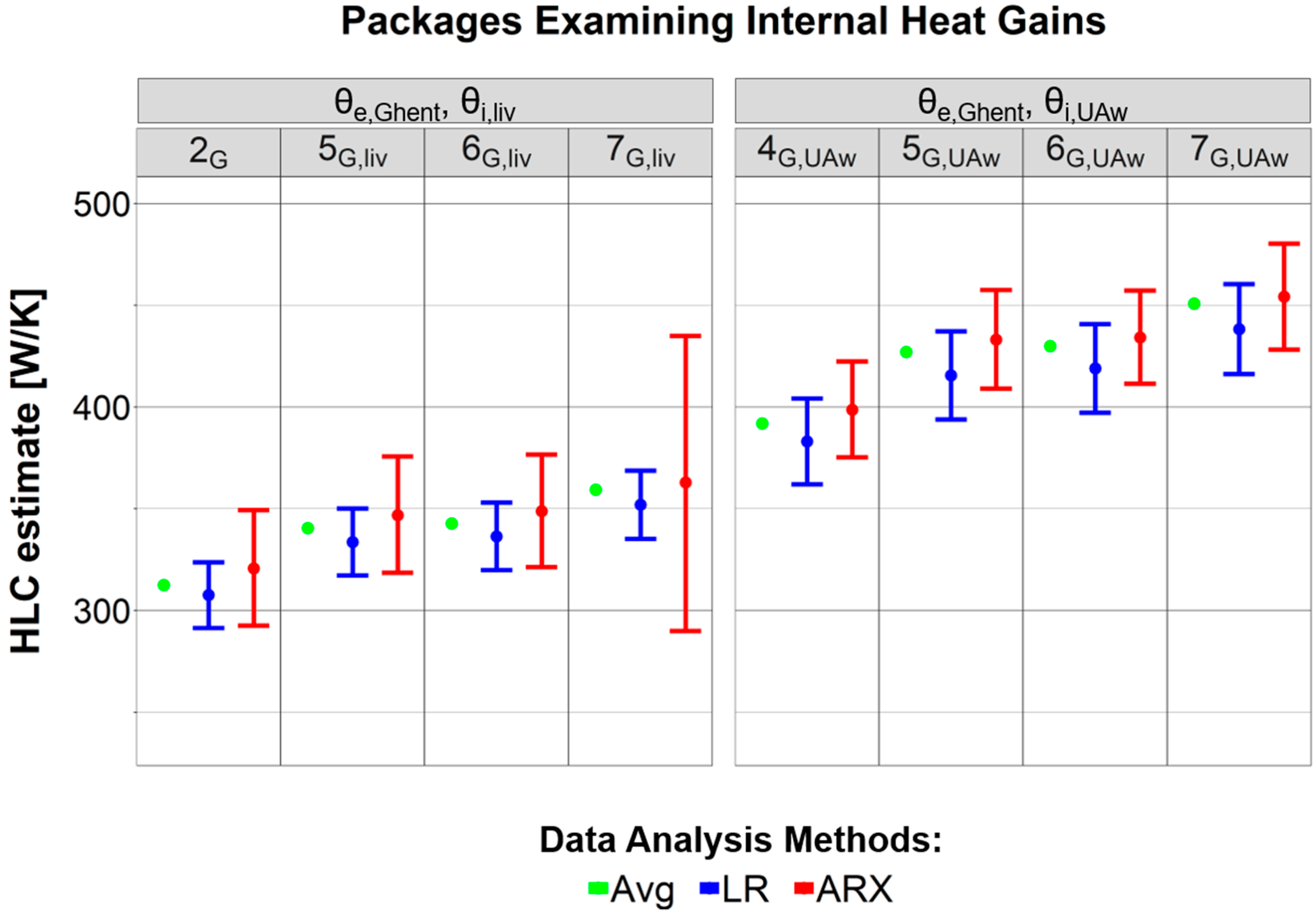
4.1.2. Impact of Representation of Internal Heat Gains

Figure 7 investigates the influence of the incorporation of the internal heat gains on the HLC estimate, and this for the data packages with θ_e,Ghent representing the exterior temperature and θ_i,liv (left side of the figure) or θ_i,UAw (right side of the figure) as the interior temperature. Hence, these packages can be found on the two left branches of the scheme in Figure 5.

From Figure 7 it can be seen that, for a given data package, the HLC estimates obtained by using the Avg, LR, and ARX methods closely correspond. The maximum difference observed between the estimates inferred by the three methods is 17.6 W/K, for package 5_G,UAw.

Data packages 2_G and 4_G,UAw neglect the internal gains.

Table 7. Specification of the input data used to represent Φ_int, for the training period.

Input Data for Φint	Elecbill (Included in 5G)	ElecOBM (Included in 6G)	ElecOBM + MHG (Included in 7G)
Mean (± σ), six-hourly data (W)	387.1 (± 0.0)	418.8 (± 327.8)	649.0 (± 337.0)
Mean (± σ), daily data (W)	387.1 (± 0.0)	418.8 (± 180.3)	649.0 (± 180.3)
Total consumption (GJ)	3.0	3.3	5.0

gives more detail on the exact input data used for Φ_int in packages 5–7. The time series Elec_bill (included in packages 5_G) and Elec_OBM (included in packages 6_G) differ on average only 31.7 W (8% of the mean value of Elec_OBM), but Elec_OBM exhibits a considerable variance. However, the results presented in Figure 7 show that, for this case, the HLC estimates are not so sensitive to the source of the data used to represent the internal heat gains. The mean estimates of packages 6_G,liv and 6_G,UAw differ maximally 0.8% from those of packages 5_G,liv and 5_G,UAw. Hence, even for the ARX models, which are identified on six-hourly data, for which the assumption of packages 5 of a constant Φ_int is more questionable, the HLC estimates thus closely correspond.

A first assumption of the metabolic heat gains (MHG) in packages 7_G learns that including these heat gains yields an additional increase of the HLC of an order of magnitude of 4.0–4.8%, compared to packages 6_G.

The presented results highlight the importance of capturing all heat sources: the HLC estimates of packages 2_G and 4_G,UAw are on average 8.5% lower than those of 6_G,liv and 6_G,UAw and 12.5% lower than those of packages 7_G,liv and 7_G,UAw. However, in some cases using a gain utilization factor of 1—thus assuming that all electricity consumption leads to useable heat gains—might be a liberal assumption [53] and the adopted MHG profile might not be entirely accurate.

The results for the setup with θ_e,Uccle are not included in Figure 7, since they show a similar increasing pattern for package 2–7 and 4–7. However, it should be noted that some of the ARX results exhibit a higher uncertainty, as depicted in Figure 8.

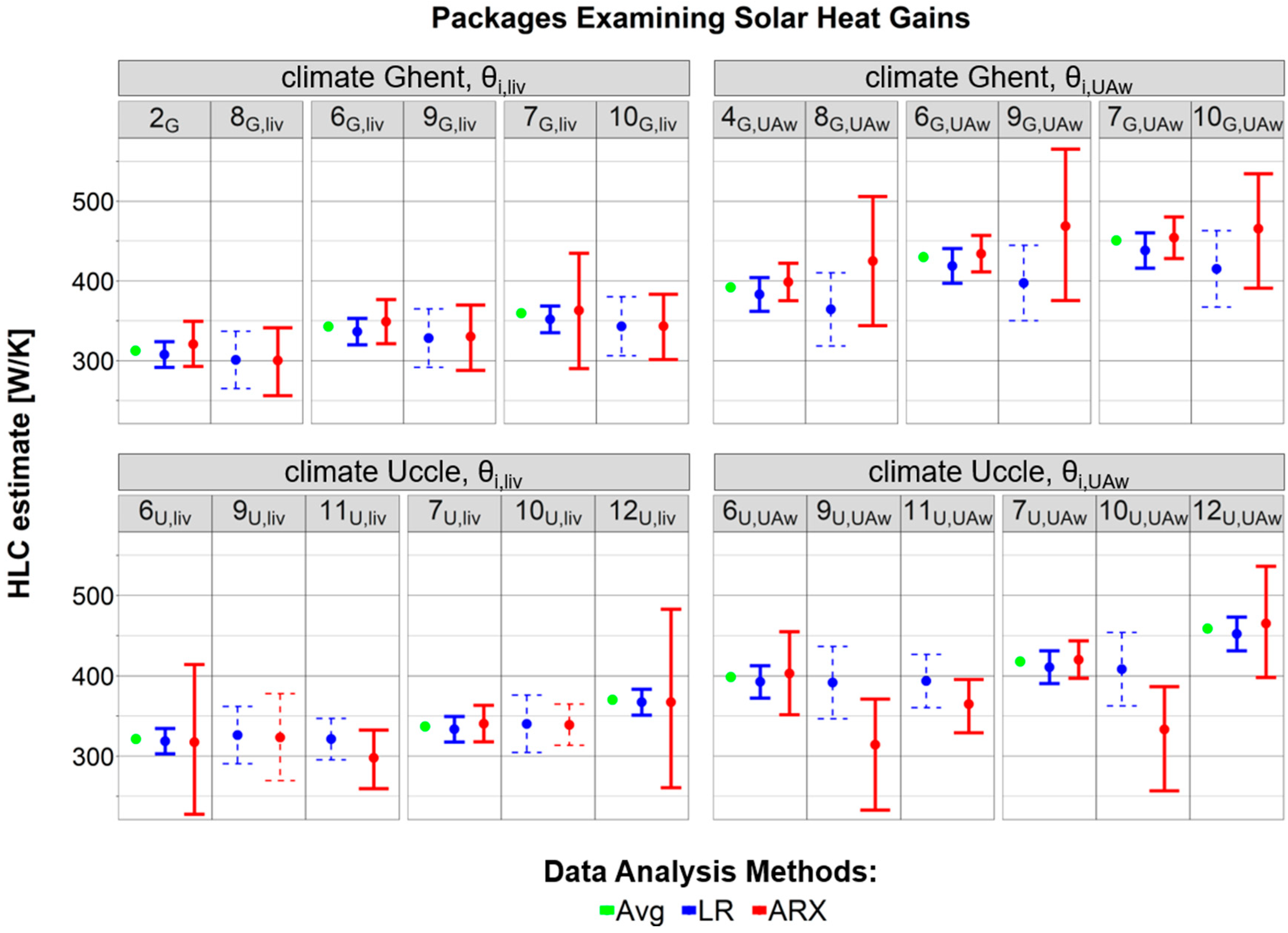
4.1.3. Impact of Representation of Solar Heat Gains

Figure 8 examines the sensitivity of the HLC estimate to the approach used to model Φ_sol.

The upper half of Figure 8 considers the climate data of the weather station located nearest to the house. It compares the results obtained when the global horizontal radiation (GHR) is monitored and Φ_sol is estimated as gA_l·GHR (packages 8–10), to the results obtained when Φ_sol is set to zero (packages 2 or 4, 6 and 7), and this for six different assumptions regarding θ_i and Φ_int. It is worth noting that none of the LR models following Equation (15) are considered valid. The dashed box plots present the results for an RST of 24 h, but these are considered untrustworthy, since the underlying models fail validation criterion (a) (Section 3.3), with gA_l being insignificant. Increasing the RST does not amend this, and for a lower RST of 12 h the model residuals do not resemble white noise (model validation criterion (b)). This issue might be caused by the coarse way in which these linear regression models try to describe the solar gains: based on daily averaged data and ignoring the gA-value’s dependency on the solar orientation and angle of incidence. Especially since solar radiation was identified as an important driver of uncertainty in the HLC characterization by Stamp et al. [54]. Moreover, the studied dwelling may be less sensitive to solar irradiance because of its relatively low window-to-wall ratio, roof overhangs, and the vegetation in front of the house (Figure 1). By contrast, the ARX models fitted on the six-hourly data do meet the adopted validation criteria. However, the extra model parameter increases the uncertainty on the HLC estimates. In addition, for the cases based on θ_i,liv, a decrease of the mean HLC estimate is observed, which seems to conflict with the fact that the assumed value for Φ_sol is raised from zero to gA_l·GHR.

The bottom half of Figure 8 shows the results when the exercise of packages 9 and 10 is repeated based on the climate data (θ_e and GHR) collected in Uccle. The mean value of GHR_Uccle over the training period is 2.4% lower than that of GHR_Ghent, and its standard deviation is nearly identical. The RMSE between both amounts to 14.8 W/m², and could for instance be caused by a time-shift in the passage of clouds. For packages 9_U and 10_U, the LR models are invalid as well, and even the ARX model fails the validation tests in the case the GHR is linked to θ_i,liv. The validation problems with the LR model do not only occur when I_sol is represented by the GHR, but also when the incident solar radiation on a vertical, south oriented plane (I_sol,S,Uccle) is used (packages 11_U). The 95% CI associated with the ARX estimates is here smaller than in the case of packages 9, but their mean estimates are again lower than those of the packages with Φ_sol set zero (6_U).

Knowledge of the GHR and the size and orientation of the windows allows to develop a simulation model to calculate the solar gains. Based on estimates of the glazing’s U-value and g-value (2.4 W/m²·K and 0.6, respectively) and without implementing any local shading, a variable ‘Q_sol,synth’ is determined that represents the dwelling’s solar heat gains. Q_sol,synth amounts to a total value of 3.8 GJ for the full training period, which corresponds to 11.3% of the measured net heat input Q_h,meter (GJ). Using the six-hourly and daily values of Φ_sol,synth (W) to represent Φ_sol (W), packages 12 estimate the HLC to be 7.9–10.7% higher than when Φ_sol was neglected in packages 7. Notably, the ARX models infer HLC values that are comparable to those assessed by the Avg and LR methods, but with wider confidence intervals. Most likely, the fast dynamics present in the real six-hourly θ_i, θ_e, Φ_h, and Φ_int data are harder to link to the synthetic solar gains.

4.1.4. Overall Impact of Input Data and Analysis Method

Packages 1 aim to assess the HLC with as little measurement data as possible; the heat output of the condensing boiler and the exterior temperature. This results in a number of fairly strong assumptions concerning for instance the interior temperature, internal gains, and solar gains. Along the tree structure in Figure 5, these were systematically replaced by more sensible and physically supported values. Ultimately, this changes the mean HLC estimate by 43.5% (package 1_G to 10_G,UAw) to 50.2% (package 1_U to 12_U,UAw)(Considering the average of the results obtained by all valid models applied on the package. For packages 1 the results of the ARX and ES models are also not taken into account.).

When ranking the aspects examined in the sensitivity analysis according to their impact on the HLC estimate, the exterior temperature signal has the lowest relative impact for the case study analyzed. Across packages 1 to 7, and only considering the valid models, a change of the mean estimate of 5.2% to 9.0% is observed when the exterior temperature signal measured at a weather station at 51 km from the site is used, instead of one registered at 4 km. (For packages 8–10 the observed deviation would reflect the cumulative impact of the difference in θ_e and GHR signal.) The LR models are consistently less influenced by the input signal used for θ_e.

Next, even for a dwelling with a WWR of 14.8%, replacing a conservative zero estimate for the solar heat gains by a value obtained from a building energy simulation, leads to a 7.9–10.7% higher mean HLC estimate. It should, though, be noted that the impact of adding Φ_sol,synth was only analyzed for two relatively extended data packages. By contrast, using the GHR as model input to represent the solar gains, results in a change of 2.5% to 22% (Considering the results of all valid models applied on packages 8–10). However, in Section 4.1.3 the reliability of these models was questioned.

From the relative difference between the results for packages 2 or 4_UAw and 7 it can be seen that measuring the energy consumption of the electrical appliances and lighting, and making a rough assumption on the MHGs, has an impact of 13.2% to 15% on the HLC estimate.

Installing temperature sensors, and combining their signals based on knowledge of the UA-values, as was done in packages 4_UAw, furthermore introduces a larger change of 18.0% to 19.6% compared to the estimate obtained based on a default assumption of 18 °C (packages 1). Finally, the largest change (23.1% to 26.9%) was observed when the UA-weighted temperature was used to represent the equivalent homogenous dwelling temperature θ_i instead of the living room temperature (considering the results of packages 4 to 7 and 12, not those of the packages where GHR was used as input).

The characterization is believed to yield more reliable estimates when the variables of the heat balance are more sensibly incorporated, as is done for the packages with higher numbers. Given the issues concerning the inclusion of the solar gains, the results for package 7_G,UAw will be considered as the ‘best guess’ based on the meteorological data of the nearest weather station. The arithmetic mean of the estimates of the Avg, LR and ARX model is here 447.7 W/K, and the 95% CIs of the LR and ARX model overlap over a range of 428.2–460.3 W/K. In addition, it should be kept in mind that incorporating the solar gains could further increase this estimate with about 42.6 W/K, as demonstrated by package 12_U,UAw (42.6 W/K is the average increase of the estimates between packages 7_U,UAw and 12_U,UAw).

For about 80% of the packages on which the Avg, LR, and ARX models were identified, the same pattern can be observed in the outcome: the ARX estimate is the highest, followed by the estimate of the Avg method. The LR estimate is on average respectively 3.4% and 1.9% lower than that of the ARX and Avg method. The ES model, and the ARX model with a constant θ_i signal, result in more deviant outcomes. Furthermore, the GHR and I_sol,S always emerged as an insignificant coefficient for the LR model.

Where in the theoretical exercise presented in [39], the ARX model yielded the most precise estimates, its outcome is here associated with the widest 95% confidence intervals. This may be related to the slightly different model fitting procedure that was applied in this study: in both cases a forward modeling procedure was adopted, but here it was chosen to only retain the significant coefficients. Furthermore, the ARX model could be more sensitive to the assumptions made than the other models, due to the higher frequency of its input data.

4.2. Comparison with Theoretical Value and Assessment of Uncertainties

Based on Equation (3), and using the values listed in Table 1, a theoretical H_tr value of 638.7 W/K is calculated. Adopting the rule of thumb proposed by Kronvall [55] that n_actual ≈ n₅₀/20 and with Q_inf = (n_actual·V)/3600 (V = internal dwelling volume) an H_inf value of 58.4 W/K is determined (Equation (2)). By summing these two values, a theoretical (arguably, this is a semi-theoretical value, because H_inf is based on an in-situ blowerdoor test) HLC value of 697.1 W/K is obtained, which is 55.7% to 51.9% higher than the values obtained via on-site characterization (the average of the estimates for packages 7_G,UAw and 12_U,UAw, respectively). However, both approaches face considerable uncertainties. Regarding the theoretical value, the following points can be made:

(a)

The U-values of the building components were determined based on assumed constructions, using default material properties. In reality, other materials than those specified in Table 1 could have been used, and the thermal conductivity and thickness of the material layers could be either higher or lower.

(b)

For the temperature ratios b_T (Equations (3) and (4)) of the floor slab above the cellar and the attic floor, constant, default values of respectively 0.8 and 0.9 were used (see Table 1). However, in reality these ratios vary over time. With the aid of the temperature signals measured in the cellar and attic it could be established that especially the temperature ratio applied to the U-value of the slab above the cellar is not appropriate in this case. Over the training period, the actual b_T values on average amount to 0.4 and 0.7 for respectively the floor slab to the cellar and the attic floor. Notably, in the calculations the variable θ_i was respectively represented by the temperature of the entrance hall and a ceiling area weighted average of the temperatures measured in the rooms on the first floor. Substituting these actual b_T values in the theoretical calculation results in an HLC value of 678.6 W/K (compared to the original value of 697.1 W/K).

(c)

According to ISO 13370 [33,34] the thermal resistance of dense concrete slabs and thin floor coverings can be neglected when calculating the U-value of the slab-on-ground floor including the effect of the ground. In this particular case, this means that the thermal resistance of the floor slab is assumed to be zero. When this suggestion is ignored, and the thermal resistances of the tiles, sand bed, and concrete slab (see Table 1) are taken into account, the U-value of the slab on ground floor lowers to 0.7 W/m²·K and the theoretical HLC to 678.5 W/K.

(d)

The surface areas in Equation (3) are calculated from building plans, the accuracy of which is unknown.

(e)

Thermal bridges have not been accounted for (Ψ and Χ in Equation (3) are assumed to be zero). However, these would only further increase the observed gap.

The impact of these five aspects on the theoretical value is however considered too limited to explain the observed discrepancy. The sensitivity analysis of the characterization based on OBM, on the other hand, also uncovered a fair number of uncertainties in this approach:

• Inappropriate sensor placement. For example, issues were raised concerning the position of the heat meter and the temperature sensors.
• Measurement errors (e.g., missing observations and small anomalies in the GHR data collected in Ghent).
• Use of unrepresentative input variables in the model: e.g., the complex search for one interior temperature signal θ_i approximating the ‘equivalent homogenous temperature’ of a multizone building.
  In this context, it could for instance be noted that the above presented OBM characterization and sensitivity analysis relied on the assumption that the temperature registered in the utility room is also representative for the former garage, where no temperature sensor was installed. Since this room has a heat loss area of 133.6 m² and is not actively heated according to the inhabitants, this assumption is questionable. To evaluate its impact on the HLC estimate, a synthetic, alternative room temperature signal is developed for the garage based on the formula expressed in Equation (31), where the subscripts ‘gar’, ‘ut’, and ‘kit’ stand for the garage, utility room and kitchen, respectively. ‘gar/ut’ indicates the building elements separating the garage from the utility room.

  $${\mathit{\theta }}_{\mathit{i},\mathit{g}\mathit{a}\mathit{r};\mathit{t}}=\raisebox{1ex}{$\left(\begin{array}{c}{{\displaystyle \sum }}_j\left(A_{gar/ut,j}·U_{gar/ut,j}\right)·{\mathit{\theta }}_{\mathit{i};\mathit{u}\mathit{t};\mathit{t}}+{{\displaystyle \sum }}_k\left(A_{gar/kit,k}·U_{gar/kit,k}\right)·{\mathit{\theta }}_{\mathit{i};\mathit{k}\mathit{i}\mathit{t};\mathit{t}}\\ +\left({{\displaystyle \sum }}_l\left(A_{gar/e,l}·U_{gar/e,l}\right)+{{\displaystyle \sum }}_m\left(A_{gar/g,m}·U_{gar/g,m}\right)\right)·{\mathit{\theta }}_{\mathit{e};\mathit{t}}\end{array}\right)$}\!\left/ \!\raisebox{-1ex}{${{\displaystyle \sum }}_n\left(A_{gar,n}·U_{gar,n}\right)$}\right..$$

  (31)

  Weighting this new temperature signal in θ_i,UAw and repeating the analysis of package 7_G,UAw yields an estimate of 501.8 W/K (average for the three methods), which is 12.1% higher than the original estimate for 7_G,UAw presented in Section 4.1. The discrepancy with the theoretical value reduces by 22%.
• Physical phenomena that are unaccounted for in the models. For packages 7 to 12 these include, for example, the opening of external doors and windows, radiative heat exchange with the sky, and latent heat gains. Other phenomena, such as the dynamic thermal loading of the building parts, internal heat gains, and solar gains, may not have been correctly incorporated.

Although these aspects might still influence the HLC estimate, it is uncertain whether these changes would explain the observed discrepancy with the theoretical value. In the meantime, retrofit measures were applied to the dwelling’s construction. Therefore, it is not possible to conduct additional measurements in order to analyze the established gap more thoroughly.

It should be emphasized that the above presented results were obtained for one particular case study dwelling and household. Moreover, the OBM data was sampled during a winter period, which is in the northern hemisphere characterized by lower exterior temperatures and solar irradiance. Hence, in order to verify whether the findings on the sensitivity of the HLC characterization can be generalized, the analyses should be repeated on other dwelling types, with a different energy performance or under other climatic conditions. Case studies on synthetic data, generated from building energy models with a known HLC, would moreover help to identify the accuracy of the different proposed OBM packages and give deeper insight into the causes of the observed gap with the theoretical HLC value.

5. Conclusions

This paper performs a systematic sensitivity analysis of the characterization of the as-built heat loss coefficient (HLC) of residential buildings based on on-board monitoring (OBM). It focuses on one specific case study dwelling and household, which were subjected to a four-month OBM campaign. By taking 35 subsets of the OBM data set and applying four different data analysis methods, it evaluates whether collecting actual OBM data on all variables of the heat balance equation is essential for the HLC characterization, or if nearly the same estimate could be inferred based on sensible assumptions.

Monitoring data of the energy use for space heating is taken as a starting point. Subsequently, the impact of adding data on the dwelling’s interior temperature, internal heat gains, and solar gains is evaluated. Firstly, using actual measurement data on the interior dwelling temperature instead of an estimated constant value, proves to have a major impact on the HLC estimate. It leads to deviations of 3.8–19.6% on the assessed HLC, depending on the number of sensors installed and the prior knowledge used to combine the signals. For this case, installing a second sensor on a different floor already causes a change of up to 14.0% compared to a single-sensor OBM setup. When monitoring the temperature in each room and combining the signals based on the rooms’ heat loss area and wall assemblies, this difference can even increase to 26.9%. Secondly, it is recommended to extend the input data package used for the characterization with information on the household’s mains electricity consumption. An up to 10.1% higher HLC estimate is obtained when the internal heat gain by appliances and lighting is approximated based on the mains electricity consumption, instead of not accounting for them. Historical cumulative consumption data and high frequency OBM data are hereby shown to be equally useful. Combined with a survey-based metabolic heat gain profile, the internal heat gain representation even yields a total increase of the HLC estimate with up to 15.0%. Thirdly, the solar heat gains are demonstrated to be hard to incorporate in the data-driven models, with the monitored global horizontal radiation often being an insignificant model input. Nevertheless, it is shown that a synthetic solar gain profile, generated via building energy simulations, can be a suitable alternative data source. Finally, the representativeness of the location of the weather station, from which the climate data is retrieved, is shown to be a point of attention. A deviation of up to 9.0% was observed on the HLC assessed using exterior temperature data from a weather station 47 km further away from the site.

Compared to the input data used, the applied data analysis method appears to have a minor, but not unimportant influence on the characterization outcome, with the HLC estimates identified through linear regression being on average 1.9% and 3.4% lower than those assessed by the Average method and ARX modeling, respectively.

A comparison of the outcome of the OBM characterization with the theoretically calculated HLC furthermore shows a significant gap between both values. By challenging some of the underlying assumptions of both approaches, such as the calculation of the U-values, use of default temperature ratios, and spatial variability of the interior temperature, suggestions are made regarding the origin of the gap.

References

1. Eurostat-Statistical Office of the European Union. Energy, Transport and Environment Indicators; Eurostat-Statistical Office of the European Union: Luxembourg, 2018. [Google Scholar] [CrossRef]
2. ISO (International Organization for Standardization). ISO 52016-1: Energy Performance of Buildings: Energy Needs for Heating and Cooling, Internal Temperatures and Sensible and Latent Heat Loads: Part 1: Calculation Procedures; International Organization for Standardization: Geneva, Switzerland, 2017. [Google Scholar]
3. Gupta, R.; Dantsiou, D. Understanding the gap between ‘as Designed’ and ‘as Built’ performance of a new low carbon housing development in UK. In Sustainability in Energy and Buildings; Hakansson, A., Höjer, M., Howlett, R.J., Jain, L.C., Eds.; Springer: Heidelberg, Germany, 2013; Volume 2, pp. 567–580. [Google Scholar]
4. Wingfield, J.; Bell, M.; Miles-Shenton, D.; Seavers, J. Elm Tree Mews Field Trial–Evaluation and Monitory of Dwellings Performance, Final Technical Report. 2011. Available online: http://www.leedsmet.ac.uk/as/cebe/projects/elmtree/elmtree_finalreport.pdf (accessed on 31 July 2019).
5. Wingfield, J.; Bell, M.; Miles-Shenton, D.; South, T.; Lowe, B. Evaluating the Impact of an Enhanced Energy Performance Standard on Load-Bearing Masonry Domestic Construction: Understanding the Gap Between Designed and Real Performance: Lessons from Stamford Brook; Leeds Beckett University: London, UK, 2011. [Google Scholar]
6. Johnston, D.; Farmer, D.; Brooke, M.; Brooke-Peat, M.; Miles-Shenton, D. Bridging the domestic building fabric performance gap. Build. Res. Inf. 2016, 44, 147–159. [Google Scholar] [CrossRef]
7. Johnston, D.; Miles-Shenton, D.; Wingfield, J.; Farmer, D.; Bell, M. Whole House Heat Loss Test Method (Coheating). 2013. Available online: https://www.leedsbeckett.ac.uk/as/cebe/projects/cebe_coheating_test_method_june2013.pdf (accessed on 31 July 2019).
8. Bauwens, G. In Situ Testing of A Building’s Overall Heat Loss Coefficient. Ph.D. Thesis, KU Leuven, Leuven Belgium, 2015. [Google Scholar]
9. Subbarao, K.; Burch, J.D.; Hancock, C.E.; Lekov, A.; Balcomb, J.D. Short-Term Energy Monitoring (STEM): Application of the PSTAR Method to a Residence in Fredericksburg, Virginia; SERI/TR-254-33 56; Solar Energy Research Institute: Golden, CO, USA, 1988. [Google Scholar]
10. Palmer, J.; Pane, G.; Bell, M.; Wingfield, J. Comparing Primary and Secondary Terms Analysis and Re-Normalisation (PStar) Test. and Co-Heating Test. Results. Final Report: BD2702; DCLG Publications: London, UK, 2011. [Google Scholar]
11. Alzetto, F.; Pandraud, G.; Fitton, R.; Heusler, I.; Sinnesbichler, H. QUB: A fast dynamic method for in-situ measurement of the whole building heat loss. Energy Build. 2018, 174, 124–133. [Google Scholar] [CrossRef]
12. Ghiaus, C.; Alzetto, F. Design of experiments for Quick U-building method for building energy performance measurement. J. Build. Perform. Simul. 2019, 12, 465–479. [Google Scholar] [CrossRef]
13. Bouchié, R.; Alzetto, F.; Brun, A.; Boisson, P.; Thebault, S. Short methodologies for in-situ assessment of the intrinsic thermal performance of the building envelope. In Proceedings of the Sustainable Places 2014 (SP2014), Nice, France, 1–3 October 2014. [Google Scholar]
14. Boisson, P.; Bouchié, R. ISABELE method: In situ assessment of the building envelope performances. In Proceedings of the Ninth International Conference on System Simulation in Buildings (SSB2014), Liege, Belgium, 10–12 December 2014; pp. 302–320. [Google Scholar]
15. Thébault, S.; Bouchié, R. Refinement of the ISABELE method regarding uncertainty quantification and thermal dynamics modelling. Energy Build. 2018, 178, 182–205. [Google Scholar] [CrossRef]
16. Senave, M.; Reynders, G.; Verbeke, S.; Saelens, D. A simulation exercise to improve building energy performance characterization via on-board monitoring. Energy Procedia 2017, 132, 969–974. [Google Scholar] [CrossRef]
17. Ljung, L. System Identification: Theory for the User, 2nd ed.; PTR Prentice Hall: Upper Saddle River, NJ, USA, 1999. [Google Scholar]
18. Madsen, H. Time Series Analysis; Chapman & Hall/CRC: Boca Raton, FL, USA, 2008; ISBN 9781420059670. [Google Scholar]
19. Jack, R.; Loveday, D.; Allinson, D.; Lomas, K. First evidence for the reliability of building co-heating tests. Build. Res. Inf. 2017, 46, 383–401. [Google Scholar] [CrossRef] [Green Version]
20. Alzetto, F.; Farmer, D.; Fitton, R.; Hughes, T.; Swan, W. Comparison of whole house heat loss test methods under controlled conditions in six distinct retrofit scenarios. Energy Build. 2018, 168, 35–41. [Google Scholar] [CrossRef] [Green Version]
21. European Commission. Benchmarking Smart Metering Deployment in the EU-27 with a Focus on Electricity; European Commission: Brussels, Belgium, 2014. [Google Scholar]
22. Annex 71 of the programme ‘‘EBC” of the IEA on ‘‘Building Energy Performance Assessment Based on In-situ Measurements”. 2016–2021. Available online: http://www.iea-ebc.org/projects/project?AnnexID=71 (accessed on 31 July 2019).
23. Castillo, L.; Enríquez, R.; Jiménez, M.J.; Heras, M.R. Dynamic integrated method based on regression and averages, applied to estimate the thermal parameters of a room in an occupied office building in Madrid. Energy Build. 2014, 81, 337–362. [Google Scholar] [CrossRef]
24. Erkoreka, A.; Garcia, E.; Martin, K.; Teres-Zubiaga, J.; Del Portillo, L. In-use office building energy characterization through basic monitoring and modelling. Energy Build. 2016, 119, 256–266. [Google Scholar] [CrossRef]
25. Uriarte, I.; Erkoreka, A.; Giraldo-Soto, C.; Martin, K.; Uriarte, A.; Eguia, P. Mathematical development of an average method for estimating the reduction of the Heat Loss Coefficient of an energetically retrofitted occupied office building. Energy Build. 2019, 192, 101–122. [Google Scholar] [CrossRef]
26. Senave, M.; Reynders, G.; Bacher, P.; Roels, S.; Verbeke, S.; Saelens, D. Towards the characterization of the heat loss coefficient via on-board monitoring: Physical interpretation of ARX model coefficients. Energy Build. 2019, 195, 180–194. [Google Scholar] [CrossRef]
27. Senave, M.; Reynders, G.; Sodagar, B.; Verbeke, S.; Saelens, D. Mapping the pitfalls in the characterisation of the heat loss coefficient from on-board monitoring data using ARX models. Energy Build. 2019, 197, 214–228. [Google Scholar] [CrossRef]
28. Chambers, J.D.; Oreszczyn, T. Deconstruct: A scalable method of as-built heat power loss coefficient inference for UK dwellings using smart meter data. Energy Build. 2019, 183, 443–453. [Google Scholar] [CrossRef]
29. De Dietrich. Modulens: Staande Hoog Rendement Ketel: AGC 15 BE-25 BE-35 BE. Available online: http://nl.dedietrich-heating.be/download/file?file=var/ddth/storage/original/application/ab3fd134254179a7081a4720c6d14a29.pdf&filename=NOT-300026053-06.pdf (accessed on 28 May 2015).
30. Cuypers, D.; Birigt Vandevelde, B.; Marlies Van Holm, B.; Stijn Verbeke, B. Belgische Woningtypologie Nationale Brochure over de TABULA Woningtypologie, 2nd ed. 2014. Available online: http://episcope.eu/fileadmin/tabula/public/docs/brochure/BE_TABULA_TypologyBrochure_VITO.pdf (accessed on 31 July 2019). (In Dutch).
31. Belgisch Staatsblad (Belgian Official Journal). Bijlage 4 bij het MB van 28 december: Transmissie Referentie Document. 2019. Available online: https://www.energiesparen.be/EPB-pedia/bijlagen-coordinatieMB#bijlage4 (accessed on 31 July 2019). (In Dutch).
32. Belgian Bureau for Standardisation (NBN). NBN EN 12831: Heating Systems in Buildings: Method for Calculation of the Design Heat Load; Belgisch instituut voor normalisatie (BIN): Brussels, Belgium, 2003. [Google Scholar]
33. ISO (International Organization for Standardization). ISO 13370: Thermal Performance of Buildings: Heat Transfer via the Ground: Calculation Methods; International Organization for Standardization: Geneva, Switzerland, 2017. [Google Scholar]
34. Schietecat, J. Warmteoverdracht Door Wanden van Gebouwen in Contact Met. de Grond. Toepassing van de Rekenmethode Uit de Norm en ISO 13370; WTCB: Brussels, Belgium, 2002. (In Dutch) [Google Scholar]
35. RENOSEEC -Collectief Renoveren, 2014–2018. Available online: http://www.renoseec.com/ (accessed on 31 July 2019).
36. De Proeftuinen van Het IWT-Duurzame ontwikkeling. Available online: https://do.vlaanderen.be/de-proeftuinen-van-het-iwt (accessed on 31 July 2019).
37. Senave, M.; Reynders, G.; Sodagar, B.; Saelens, D. Uncertainty in building energy performance characterization: Impact of gas consumption decomposition on estimated heat loss coefficient. In Proceedings of the 7th International Building Physics Conference. (IBPC 2018), Syracuse, NY, USA, 23–26 September 2018; pp. 1491–1496. [Google Scholar]
38. Bureau for Standardisation (NBN). NBN EN ISO 9972: Thermische Eigenschappen van Gebouwen: Bepaling van de Luchtdoorlatendheid van Gebouwen: Overdrukmethode Met. Ventilator; Belgisch instituut voor normalisatie (BIN): Brussels, Belgium, 2015. (In Dutch) [Google Scholar]
39. Senave, M.; Roels, S.; Reynders, G.; Verbeke, S.; Saelens, D. Assessment of data analysis methods to identify the heat loss coefficient from on-board monitoring data. Energy Build. 2019. submitted for publication. [Google Scholar]
40. ISO (International Organization for Standardization). ISO 9869-1: Thermal Insulation: Building Elements: In-situ Measurement of Thermal Resistance and Thermal Transmittance: Part. 1: Heat Flow Meter Method; International Organization for Standardization: Geneva, Switzerland, 2014. [Google Scholar]
41. Bauwens, G.; Roels, S. Co-heating test: A state-of-the-art. Energy Build. 2014, 82, 163–172. [Google Scholar] [CrossRef]
42. Ghiaus, C. Experimental estimation of building energy performance by robust regression. Energy Build. 2006, 38, 582–587. [Google Scholar] [CrossRef]
43. Janssens, A. IEA EBC Annex 58: Report of Subtask 1b: Overview of Methods to Analyse Dynamic Data; KU Leuven: Leuven, Belgium, 2016. [Google Scholar]
44. Madsen, H.; Bacher, P.; Bauwens, G.; Deconinck, A.H.; Reynders, G.; Roels, S.; Himpe, E.; Lethé, G. IEA EBC Annex 58: Report of Subtask 3, part 2: Thermal Performance Characterisation Using Time Series Data–Statistical Guidelines; KU Leuven: Leuven, Belgium, 2016. [Google Scholar]
45. Belgisch Staatsblad (Belgian Official Journal). Bijlage 5 bij het energiebesluit: Bepalingsmethode EPW: Bepalingsmethode van het peil van primair energieverbruik van residentiële eenheden. 2019. Available online: https://www.energiesparen.be/EPB-pedia/regelgeving/energiebesluit/bijlageV (accessed on 31 July 2019). (In Dutch).
46. ISO (International Organization for Standardization). ISO 8996: Ergonomics of the Thermal Environment: Determination of Metabolic rate; International Organization for Standardization: Geneva, Switzerland, 2004. [Google Scholar]
47. Klein, S.A.; Beckman, W.A.; Mitchell, J.W.; Duffie, J.A.; Duffie, N.A.; Freeman, T.L.; Kummer, J.P. TRNSYS 17: A Transient System Simulation Program; Solar Energy Laboratory, University of Wisconsin: Madison, WI, USA, 2009; Available online: http://sel.me.wisc.edu/trnsys (accessed on 31 July 2019).
48. Klein, S.A.; Beckman, W.A.; Mitchell, J.W.; Duffie, J.A.; Duffie, N.A.; Freeman, T.L.; Mitchell, J.C.; Braun, J.E.; Evans, B.L.; Kunmmer, J.P.; et al. TRNSYS 17: A Transient System Simulation Program: Volume 4: Mathematical Reference; Solar Energy Laboratory, University of Wisconsin: Madison, WI, USA, 2014. [Google Scholar]
49. R Core Team. R: A Language and Environment for Statistical Computing; R Foundation for Statistical Computing: Vienna, Austria, 2017; Available online: https://www.r-project.org/ (accessed on 31 July 2019).
50. R-core. lm: Fitting Linear Models. Available online: https://www.rdocumentation.org/packages/stats/versions/3.4.3/topics/lm (accessed on 31 July 2019).
51. Jiménez, M.J.; Madsen, H.; Andersen, K.K. Identification of the main thermal characteristics of building components using MATLAB. Build. Environ. 2008, 43, 170–180. [Google Scholar] [CrossRef]
52. Efron, B.; Tibshirani, R. Bootstrap methods for standard errors, confidence intervals, and other measures of statistical accuracy. Stat. Sci. 1986, 1, 54–75. [Google Scholar] [CrossRef]
53. Suszanowicz, D. Internal heat gain from different light sources in the building lighting systems. In E3S Web of Conferences; EDP Sciences: Yulis, France, 2017; Volume 19, p. 01024. [Google Scholar]
54. Stamp, S.; Lowe, R.; Altamirano-Medina, H. Using simulated co-heating tests to understand weather driven sources of uncertainty within the co-heating test method. In Proceedings of the ECEEE 2013 Summer Study, Toulon/Hyères, France, 3–8 June 2013; pp. 2049–2055. [Google Scholar]
55. Kronvall, J. Testing of houses for air leakage using a pressure method. ASHRAE Trans. 1978, 84, 72–79. [Google Scholar]
Figure 1. Front facade (left) and back facade (right) of the case study building.
Energies 12 03322 g001
Figure 2. Floor plans of the case study building, with (1) entrance hall with cloakroom and toilet, (2) study, (3) living room, (4) kitchen, (5) utility room, (6) former garage used as storage space, (7) landing, (8)–(10) bedrooms, and (11) bathroom. The X marks indicate the locations of the interior temperature sensors (see Section 2.2). The building fabric of which the heat loss coefficient (HLC) will be assessed, is colored red.
Energies 12 03322 g002
Figure 3. Cross sections AA′ (left) and BB′ (right). The building fabric of which the HLC will be assessed, is colored red.
Energies 12 03322 g003
Figure 4. Time series plots of the collected monitoring data for five typical days at the beginning of January 2017. The abbreviations ‘liv’ and ‘bed’ stand for, respectively, the ‘living room’ (No. 3 in Figure 2) and the master ‘bedroom’ (No. 9 in Figure 2). Figures display hourly values.
Energies 12 03322 g004
Figure 5. Schematic representation of the input data packages used in the sensitivity analysis. The abbreviations ‘liv’, ‘bed’, and ‘MHG’ stand for, respectively, ‘living room’, ‘bedroom’, and ‘metabolic heat gains’. Table 4 further details the content of the packages.
Energies 12 03322 g005
Figure 6. HLC estimates obtained by applying the Average (Avg), Linear Regression (LR) and Energy Signature (ES) method, as well as an ARX model, on the data packages investigating the influence of the considered interior temperature. The dots indicate the mean estimates, and the whiskers represent the 95% confidence intervals.
Energies 12 03322 g006
Figure 7. HLC estimates obtained by applying the Average method (Avg), Linear Regression (LR), and an ARX model on the data packages investigating the influence of the incorporation and representation of the internal heat gains. The dots indicate the mean estimates, and the whiskers represent the 95% confidence intervals.
Energies 12 03322 g007
Figure 8. HLC estimates obtained by applying the Average method (Avg), Linear Regression (LR), and an ARX model on the data packages investigating the influence of the incorporation and representation of the solar gains. The dots indicate the mean estimates, and the whiskers represent the 95% confidence intervals. The outcome of models that are considered invalid are shown dashed.
Energies 12 03322 g008