Model Analysis of Electrically Driven Vehicles by Means of Unknown Input Observers

Abstract

The article describes a method to analyze the powertrain operation of electrically driven vehicles in cases of insufficient information (i.e., unknown control algorithms, no torque measurements during vehicle tests). The method implies mathematical modeling with involvement of so-called unknown input observers. A variant of such an observer is proposed. Using that observer, studies of a hybrid vehicle and a pure electric vehicle are performed. The models with torque observers simulated tests of said vehicles conducted on a chassis dynamometer and on roads. For the hybrid vehicle, operating regimes of main powertrain components were identified. For the electric vehicle, the identification revealed a coordinated operation of regenerative braking and mechanical braking. Adequacy of the modeling, including identification of the unmeasured torques, was verified through a comparison with experimental data.

1. Introduction

Development and enhancement of electrically driven vehicles, either hybrid or pure electric, implies a good understanding of properties possessed by powertrains of these vehicles. One of the possible ways towards such understanding is to study commercially available vehicles of said types, as well as powertrains thereof. A broad variety of such vehicles offered by a number of manufacturers is favorable for practicing of this approach. A number of descriptions of such studies can be found, for example, in the works by Argonne National Laboratory (ANL, USA) [1,2,3]. Besides vehicle testing and analysis of testing results, these works include modeling aimed at replication of the conducted tests. The most valuable results obtained from that modeling are operating regimes of powertrain components defined by their operating points. The latter constitute combinations of no less than two operating parameters of the component at hand. For example, for an internal combustion engine (ICE) and electric machines (EM), operating points include rpms and torque. Operating points may also include fuel rate and exhaust emissions (for an ICE), efficiency, operating temperature, and so forth. Analysis of operating points allows making observations and drawing conclusions about powertrain’s efficiency and ecology-related properties as well as its controls and the optimality thereof.

In References [2,3], one can find examples of such researches having Toyota Prius cars as the studied objects. In these works, the control algorithms of hybrid powertrains were replicated from the descriptions found in the literature available on the Prius powertrain. In the simulations conducted, the same vehicle parameters and velocity patterns were employed as in the laboratory tests performed prior to the simulations. Being useful and efficient, this approach nevertheless has its limitations. The main limitation is the lack of information on control algorithms used in powertrains of commercially available vehicles. Although the control algorithm of the Toyota Hybrid System is described by the manufacturer [4], this can be considered as a rare case of such detailed description available, because control systems usually constitute a property of their developers or vehicle’s manufacturers being protected or otherwise not available for reading.

With the control algorithm of the studied powertrain unknown, a researcher may identify operating points of powertrain components by means of direct measurements of all relevant parameters. The problem is such comprehensive measurements may not be technically affordable. One of the “hard-to-measure” parameters is the shaft torque of internal combustion engines and electric machines. If there is no opportunity of reading a torque from the powertrain’s CAN bus, this torque should be measured by a transducer placed between the driving unit (ICE or EM) shaft and the transmission shaft driven by this unit. Even if a researcher is authorized for such interventions into the vehicle’s structure, mounting of torque transducers may constitute a difficult and time-consuming task. Therefore, this approach is more feasible in the case of studying few vehicles, than in the case when many objects should be studied. However, even this complicated approach may not be affordable if the vehicle is provided to the researcher with no authorization for interventions into its inner structure.

In order to work around the described complications, one may resort to indirect identification of powertrain operational parameters, which cannot be measured. This can be accomplished by employing mathematical tools, which, in control theory, are called observers. Usually, observers are based on (or derived from) mathematical models of objects, whose variables are to be identified. The measured quantities are fed into the observer, which calculates and outputs the unmeasured ones. Observers of state variables, such as the Luenberger’s observer [5] and the Kalman filter [6,7,8], have found a wide use in engineering applications. However, these observers cannot be directly applied for estimation of unmeasured torques, since the latter constitute the input (or control) variables rather than the state ones. This type of variable requires using so called unknown input observers [9,10,11] (hereafter abbreviated UIO) for identification, which constitute a relatively new kind of observer.

2. Analysis of Unknown Input Observers. Elaboration of the Observer Design

Analysis of the unknown input observers described in the literature shows that a part of them is derived from the Luenberger’s state observer. The latter is applied to the objects, which can be described by the standard linear state–space form. In order to compensate stochastic unmeasured disturbances, a linear correction of observation error is introduced with an adjustable vector gain $k_1$:

$$\{\begin{array}{l}\dot{\widehat{x}}=A\widehat{x}+Bu+k_1\left(y-\widehat{y}\right)\hfill \\ \widehat{y}=C\widehat{x}+Du\hfill \end{array}$$

(1)

where $x$, $u$, and $y$ are state, control, and output variables, respectively; symbols “^” denote estimates of the variables. A, B, C, and D are the matrices (or vectors) of object’s parameters assumed to be known, at least approximately. Unlike control applications where some uncertainty of plant’s parameters usually takes place, in researches, these can be estimated with a good precision.

In order to derive an UIO from this observer, the system is transformed as follows. The state variable x becomes observable and is treated as the output of the system. The control variable u becomes unobservable and is expressed as a function of the state (output) observation error:

$$\{\begin{array}{l}\dot{\widehat{x}}=A\widehat{x}+B\widehat{u}+k_1\left(x-\widehat{x}\right)\hfill \\ \dot{\widehat{u}}=k_2\left(x-\widehat{x}\right)\hfill \end{array}$$

(2)

Examples of using this observer for identification of unmeasured torques within the vehicle driveline are given in References [9,11].

However, the structure of the described UIO is not free from shortcomings. Note that in the original Luenberger’s observer, the $k_1$ gain is only intended for compensation of disturbances (i.e., parameter estimation errors and measurement noise). In the examples given in References [9,11], this gain becomes a part of the function, which calculates unknown input variables. This implies having that gain rather high, which increases influence of the corresponding term, bringing it beyond the disturbance rejection role. Having a substantial effect on the model dynamics, this term, however, does not have any physical equivalent in the modeled object, which may diminish both the adequacy of the model and the estimation of the unmeasured variables. The second question about the described UIO relates to the expression calculating the input variable estimate being an integral of the state estimation error $x-\widehat{x}$. This integral term may introduce an oscillatory behavior into the model if its gain $k_2$ is increased in order to minimize the estimation error. Damping of these oscillations may be performed by increasing the $k_1$ gain, however, as it was mentioned above, this will deteriorate model adequacy.

In order to overcome the described problematic issues, a modification of the UIO can be proposed, which does not alter the modeled object structure and allows for increasing the gains in order to minimize the state estimation error, while suppressing oscillations in the input variable estimate signal. The concept of this modified observer can be explained by means of an analogy between the unknown input estimation task and the task of modeling vehicle linear motion with a predetermined velocity pattern. It is known that there are two ways of solving this task, namely, the back-facing approach, and the forward-facing approach [12].

The former approach implies calculation of operating points “from the wheels towards the engine shaft”. Vehicle speed specified by a driving cycle allows for the use of the known velocity-dependent functions for calculation of the steady speed resistance forces (rolling resistance and air drag), while vehicle acceleration and mass are used to calculate the dynamic resistance force (i.e., inertia force). Using an inverse transfer function of the transmission (inverse gear ratios and efficiency) the full resistance force and the vehicle speed are converted into corresponding engine torque and shaft speed, which determine engine operating point allowing for calculation of such quantities as the fuel rate and exhaust emissions.

The forward-facing approach implies direct solving of equations of the vehicle dynamics. Control signal (throttle or torque) is generated by the engine model and converted by a direct transfer function of the transmission into the wheel force. The latter is applied to the mass of the vehicle alongside with the velocity-dependent steady speed resistance forces, which brings the vehicle mass into motion. In order to make this model track a driving cycle schedule, a closed loop control of the input signal is implemented by means of a regulator, which uses the required velocity as the command and the actual velocity (calculated by the vehicle model) as the feedback.

In the forward-facing modeling, a driving cycle schedule can be replaced by a velocity signal logged during a test of an actual vehicle—either on a chassis dynamometer or on a road. In that case, the task can be qualified as “identification of powertrain operating regimes based on experimental data”. Furthermore, this task may be expanded on the case of a powertrain with few degrees of freedom (for example, a powertrain comprising a continuously variable transmission) and a powertrain with several driving units (a hybrid powertrain or individual-wheel drive powertrain). Solving this task implies attaching a regulator to the torque-input of each powertrain component model, which operating regime should be identified. A controlled variable should be assigned to each regulator. The feedback value of this variable is calculated by the powertrain model, and the command value is taken from experimental data. By compensating the difference between the command and the feedback signal, the regulator calculates non-measured torque.

A general condition making such torque estimation correct is the adequacy of the model, which the observer is based on. In turn, the model adequacy depends on the accuracy of defining its parameters (vehicle mass, gear ratios, and so forth) and the resistance forces, which are recommended to be calculated from experimental data (for example, from coasting test results). The best way to verify the observer design is a check measurement of the torque this observer identifies. However, such checking may not be affordable, and in this case, one can resort to an oblique verification (proving the correctness of the identification rather than its precision) based on accuracy of calculation of variables, which relate to the identified torques indirectly. For instance, in the above-described case of using a torque observer in order to identify operating points of the ICE in a driving cycle, a comparison of calculated and measured engine fuel rate can be used as an indirect indication that operating regimes were estimated correctly.

The next two sections describe case studies in which the proposed observer was used in order to investigate powertrain operation of electrically driven vehicles. In these examples, observers were designed taking into account the functions investigated, the powertrain components involved in performing these functions, and the experimental data available.

3. Case Study-1. Electric Vehicle with a Regenerative Braking System

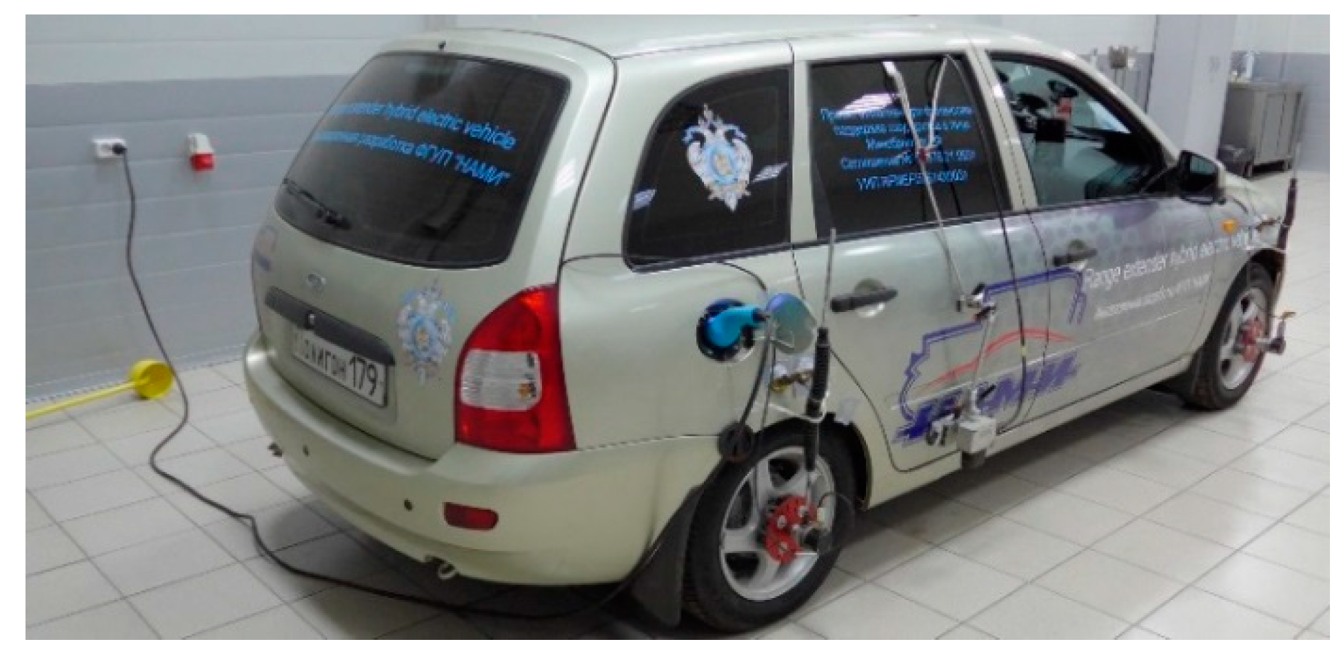
The object of the study was an electric vehicle augmented with a range extender unit (see Figure 1) [13,14]. It is equipped with a regenerative braking system, which operates in the full vehicle deceleration range, up to emergency braking, and in accordance with UNECE Regulation 13-H, belongs to the “B” category of regenerative braking systems. This category implies regenerative braking to be activated by the brake pedal, which requires a coordinated operation of the traction electric drive and the service braking system as well as an appropriate response of regenerative braking system to interventions of active safety systems. In the literature, such coordinated operation is called “torque blending” [15]. Elaboration of this function constitutes the most difficult part of regenerative braking system development, which makes its investigation particularly important [15,16,17,18,19].

For the study of the regenerative braking system, the following tasks were formulated: conduct tests of the studied vehicle in order to identify the main parameters for its model; conduct tests, in which the regenerative braking function engages and operates throughout its full operational range; and based on the test results, identify braking torque distribution between the electric drive and the brake mechanisms. Among the questions of interest were the deceleration range of pure regenerative braking and interaction between the regenerative braking system and the antilock braking system (ABS). Investigation of these issues was complicated by unavailability of torque measurements. Therefore, in order to define operating points of the studied system, a torque observing structure had to be elaborated.

The main feature of torque identification in the described braking system is a necessity of calculating torques exerted by three devices, namely, the traction electric motor, the front brake mechanisms (considered as a single mechanism), and the rear brake mechanisms (also considered as a single mechanism). However, when attached to the model, an observer of the above-described design will identify torque in a certain place of the driveline rather than torque of the specific device. Therefore, the observers should be placed in a way that allows the identified torques to be assigned to the three mentioned devices (or splitting the identified torques between these devices). The chosen places were the traction EM shaft, the front wheels, and the rear wheels. Additionally, three independent variables are to be chosen as inputs of the observers. Each of these variables should be both logged during the experiments and calculated by the vehicle model. An evident choice of the inputs for the torque observers attached to the wheels are angular speeds (or rpms) of those wheels, which can be easily measured during tests. Although the EM shaft speed also can be measured, it is not suitable as an observer input, since it is proportional to the angular speed of the front wheels, which are connected to the EM shaft by a fixed-ratio final drive. Other measured quantities associated (although not directly) with operation of the traction electric drive are current and voltage of the traction battery. Since dynamics of current is simpler than that of voltage, the former is more suitable as an observer input. Note that such an observer requires efficiency of the traction electric drive to be taken into account. In the case the latter is not known, it can be identified (at least in some operating points of the EM) by the torque observers using the method described below. 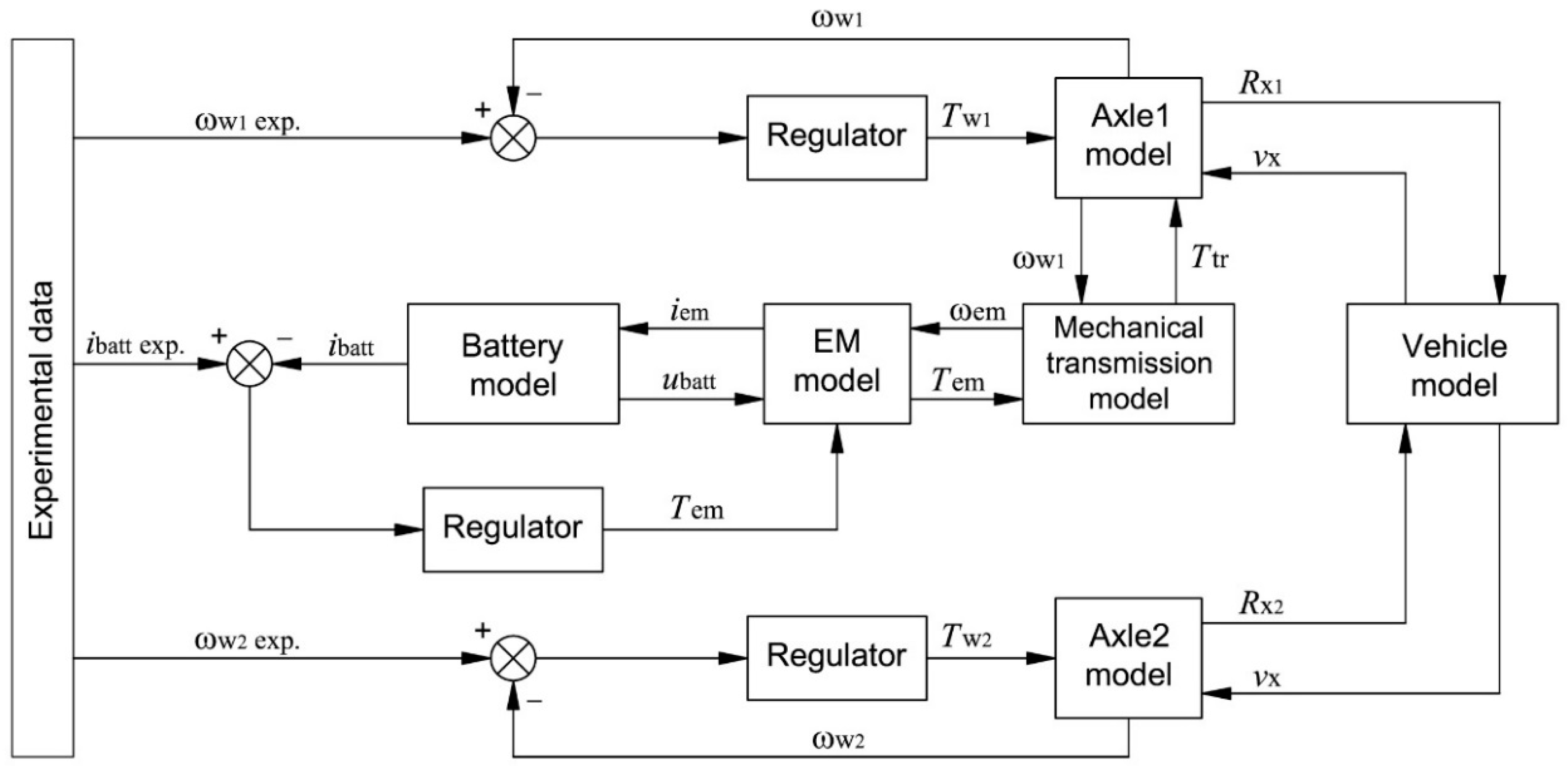Figure 2 shows the structure of the torque observation system elaborated for the studied vehicle and its regenerative braking system. All the observers in this system employ PI regulators for calculation of the non-measured torques. The designations of variables shown in this figure are explained in the formulae below. “Axle 1” and “Axle 2” stand for the front (driving) and rear (driven) axles respectively.

In accordance with the torque observation structure elaborated, the model of vehicle dynamics, besides its linear motion (the road is assumed horizontal), should calculate independent rotation of the front and the rear wheels. The equation of wheel rotational dynamics includes the wheel torque, the counteracting moment created by the tire force, and the rolling resistance moment. The model derived from these assumptions constitutes the following system of equations:

$$\{\begin{array}{l}\left(T_{em}-{ℐ}_{em}·{\dot{\omega }}_{em}\right)·u_0-T_{mech,drag1}=T_{tr}\\ T_{tr}-T_{brake1}=T_{w1}\\ -T_{mech,drag2}-T_{brake2}=T_{w2}\\ {ℐ}_w·{\dot{\omega }}_{w1}=T_{w1}-R_{x1}·r_{w1}-M_{f1}\\ {ℐ}_w·{\dot{\omega }}_{w2}=T_{w2}-R_{x2}·r_{w2}-M_{f2}\\ m_v·{\dot{v}}_x=R_{x1}+R_{x2}-F_{air}\end{array}$$

(3)

where $T_{em}$, ${\omega }_{em}$, and ${ℐ}_{em}$ are respectively electric machine shaft torque, shaft speed, and rotor inertia; $u_0$ is the speed ratio of the final drive; $T_{mech,drag}$ is the drag torque within the mechanical transmission; $T_{tr}$ is the output torque of the mechanical transmission; $T_{brake}$ is the torque exerted by a “lumped” brake mechanism; $T_w$, ${\omega }_w$, and ${ℐ}_w$ are respectively wheel torque (per axle), angular speed, and inertia (per axle); $R_x$ is the longitudinal tire force (per axle); $M_f$ is the tire rolling resistance moment (per axle); $m_v$ is the vehicle mass; $v_x$ is the vehicle longitudinal velocity; $F_{air}$ is the air drag force. Indices 1 and 2 denote the front wheel axle and the rear wheel axle respectively.

The tire longitudinal force constitutes a product of the normal force ($R_z$) and the longitudinal adhesion coefficient (${\mu }_x$): $R_x=R_z·{\mu }_x$. The normal forces per axle are calculated from static force equilibrium of the vehicle. A tire model is employed for calculation of adhesion coefficients. Typically, this coefficient is represented as a function of the tire slip, which in this work is calculated by the following expression [20]:

$$S_x=-\left(1-\frac{{\omega }_w·r_{e0}}{v_x}\right),$$

(4)

where $r_{e0}$ is the effective rolling radius calculated as a quotient of $v_x$ and ${\omega }_w$ when the wheel is in the free-rolling mode [20].

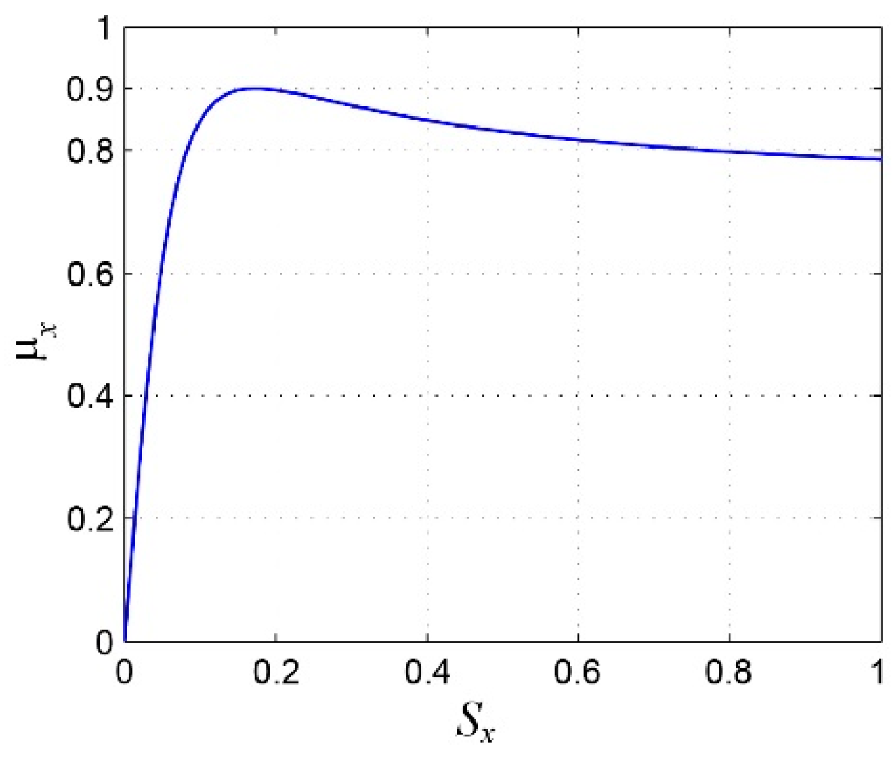
A well-known tire model called the Magic Formula (MF) [20] was employed as the approximating function for ${\mu }_x\left(S_x\right)$. This model constitutes a set of unified trigonometric functions describing all relevant factors influencing tire-road adhesion. An expression approximating the longitudinal adhesion reads as follows:

$${\mu }_x=D_x·\sin \left(C_x·arctan\left(B_x·S_x-E_x\left(B_x·S_x-arctan\left(B_x·S_x\right)\right)\right)\right),$$

(5)

where $D_x$ defines the ${\mu }_{x,max}$, and $B_x$, $C_x$, and $E_x$ define the shape of the normalized ${\mu }_x\left(S_x\right)$ curve.

It is obvious that estimation accuracy of the tire–road adhesion is one of the major factors influencing the correctness of wheel torques estimation. For the studied vehicle, another factor is determined by its front-wheel drive powertrain, which implies that in the traction mode, the rear wheel torque observer should identify a torque lying in the vicinity of zero. Adjustment of the observers and the vehicle dynamics model showed that this condition is affected by the adhesion characteristics and effective rolling radii of the front and rear tires.

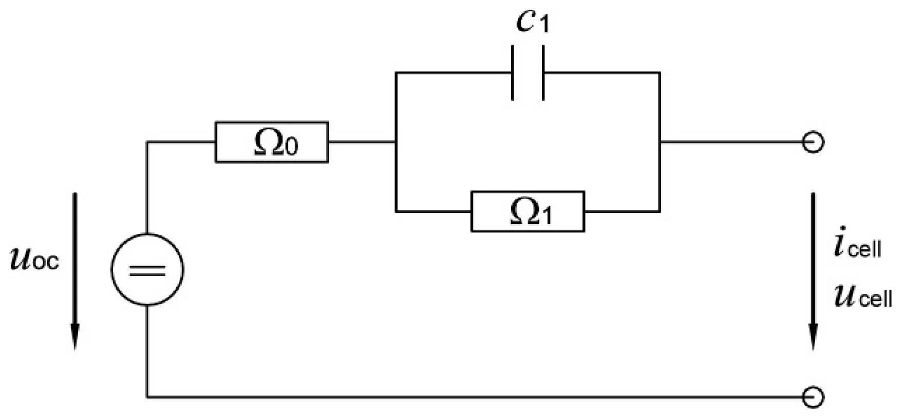
In the powertrain model, the traction battery current used for identification of the EM torque should be calculated alongside the battery voltage. This implies using a battery model. In studies of electrically driven vehicles, a prevailing approach of calculating the electrical parameters of traction batteries is equivalent circuit modeling [12,21,22]. A battery equivalent circuit simulates voltage response to a current load. In this work, a relatively simple circuit (Figure 3) was employed, which includes an open-circuit voltage source $u_{oc}$ (i.e., no-load voltage characteristic), internal resistance ${\Omega }_0$, and a voltage filter, which consists of a capacitor $c_1$ and a resistor ${\Omega }_1$ and is intended for improving accuracy of calculating voltage transients. Applying Kirchhoff’s voltage and current laws to this circuit allows to derive the following equation system, being a mathematical model of an “average” accumulator cell of the traction battery:

$$\{\begin{array}{l}{\dot{u}}_1=\frac{i_{cell}·{\Omega }_1-u_1}{{\Omega }_1·c_1}\hfill \\ u_{cell}=u_{oc}-i_{cell}·{\Omega }_0-u_1\hfill \end{array}$$

(6)

where $i_{cell}$ and $u_{cell}$ are cell current and voltage respectively. Since all the cells of the considered traction battery are connected in series, the battery current ($i_{batt}$) is equal to that of an “average” accumulator cell. Multiplying the cell voltage by the number of cells yields the traction battery voltage ($u_{batt}$).

In accordance with the elaborated observing structure, the following measuring equipment was installed in the tested vehicle: wheel rpm sensors, current and voltage sensors of the traction battery (battery management system’s sensors), vehicle longitudinal velocity, and acceleration sensors. Prior to the regenerative braking tests, auxiliary tests were conducted in order to define the main parameters used for modeling. In particular, a number of coast-down tests were performed, which allowed calculating the total steady-speed resistance force as a function of the vehicle velocity. Additional chassis dynamometer coast-down tests allowed to identify the resistance of the driving axis, which consists of the transmission drag torque and the rolling resistance of the front tires. Vehicle weight distribution and the center of gravity height were acquired by a weighing testbed.

Regenerative braking tests were conducted at the dry, horizontal asphalt road and consisted of “triangle” velocity patterns, i.e., acceleration phase up to 80 km/h, then braking phase with a constant deceleration magnitude. The latter was increased from test to test in a stepwise manner up to ABS intervention. After each test run, the temperature of the brake mechanisms was measured. This allowed to identify a deceleration magnitude, at which the torque blending begins (i.e., mechanical braking begins adding to the regenerative braking).

Identification of the tire–road adhesion characteristics was conducted by means of the vehicle test data, the model of vehicle dynamics, and the torque observation system. Identification implied simulations of the road tests, in which ABS interventions took place. In these experiments, the tire–road adhesion was approaching its maximum value, which allows identifying $D_x$ coefficient of the MF model. The simulations were conducted with the wheel torque observers only—there was no need in the EM torque observer. Other MF coefficients were adjusted in the way providing minimum model errors of the vehicle velocity and acceleration, which were compared to those measured during the tests. 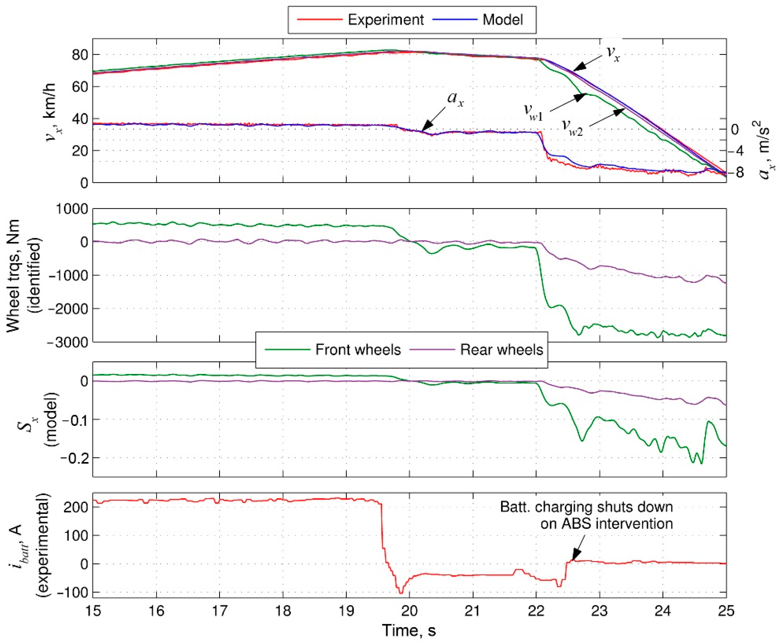Figure 4 shows the simulation results with minimum model errors obtained; Figure 5 shows the corresponding tire–road adhesion characteristic. In addition to the vehicle velocity $v_x$, the upper plot shows the linear velocities of the front and rear wheels denoted $v_{w1}$ and $v_{w2}$ respectively. (The latter almost coincides with $v_x$). Adjusting the MF coefficients and tire effective rolling radii allowed to meet one of the identification correctness criteria, namely, near-zero torque seen at the rear wheels.

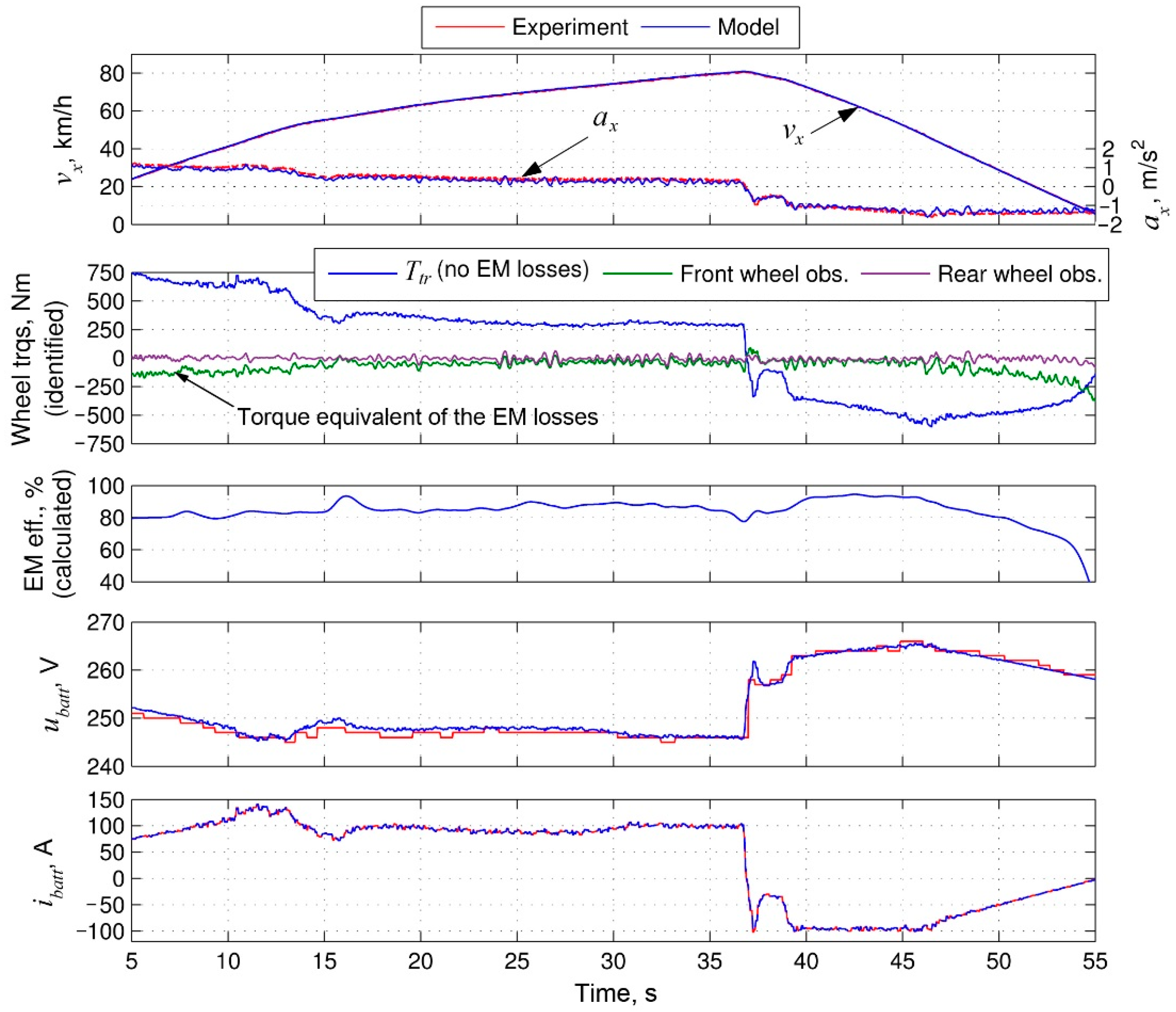
At the next step of the study, a simulation was conducted replicating the test where the maximum deceleration provided by the pure regenerative braking was achieved. In this simulation, all the torque observers were active. However, the model of the traction electric drive did not include power losses. Assuming that the losses in the electric drive can be expressed as an equivalent drag torque ($T_{em}^{loss}$) acting within the transmission, one can arrive at the following torque equilibrium: $T_w=(T_{em}^{noloss}-T_{em}^{loss})u_0-T_{mech,drag1}$. With $T_{em}^{noloss}·u_0$ identified by the EM-torque observer and $T_{mech,drag1}$ defined from the experimental data, the torque observer attached to the front wheels will calculate the difference between these and $T_w$, i.e., $T_{em}^{loss}·u_0$. Having this torque calculated, one can obtain the electric drive efficiency using the following formula:

$${\eta }_{em}={\left(\frac{T_{em}^{loss}·u_0·{\omega }_{w1}}{i_{batt}·u_{batt}}\right)}^{sgn\left(T_{em}^{noloss}\right)}$$

(7)

where $sgn\left(T_{em}^{noloss}\right)$ is introduced for the generation mode, in which the expression in brackets becomes equal to $1/{\eta }_{em}$ and therefore needs to be raised to the power of −1 (in the generation mode, $T_{em}^{noloss}<0$).

Figure 6 shows simulation results including the calculated electric drive efficiency. Since in this experiment the electric machine exerts the maximum braking torque allowed by its control system, the obtained efficiency can be used in other simulations with the same EM torque attained, i.e., in the experiments with torque blending, where the maximum EM torque is added with torque of the brake mechanisms.

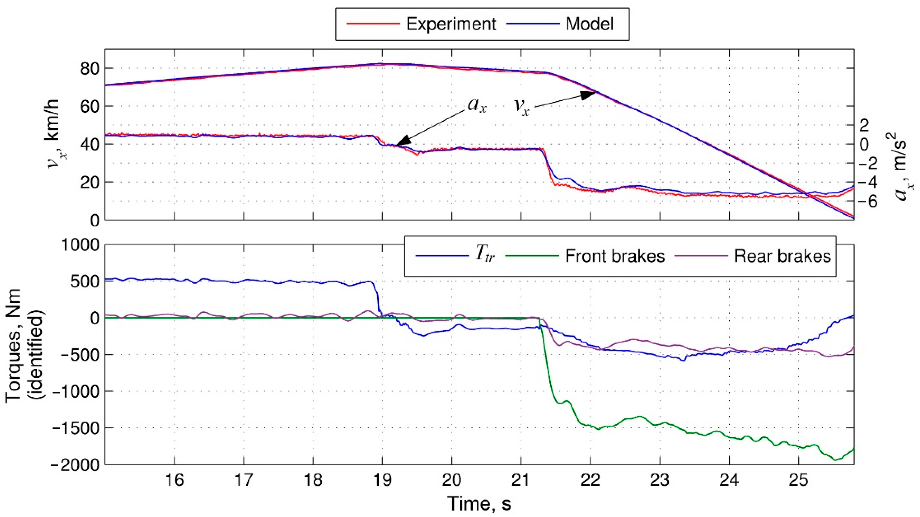
At the third step of the study, an experiment with the “torque blending” was simulated. All the torque observers were active, and the efficiency of the electric drive obtained at the previous step was taken into account. Since $T_{em}^{loss}$ was included in $T_{em}$, the torque observer connected to the front wheels was identifying torque of the brake mechanisms. The simulation results are shown in Figure 7.

Deviations between the calculated and experimental data obtained in the presented simulations can be divided into two types. The first one corresponds to regulator tracking errors. These are defined by regulator gain values, which should be adjusted so as to provide a balance between the tracking precision and the quality of transient behavior (i.e., preventing oscillations or excessive magnitude of the control signal). The second type corresponds to modeling errors, i.e., accuracy of the model used. Note that regulator tracking precision also contributes to this accuracy, since the control signals are included in the modeling loop.

In the simulations conducted, the following relative mean square tracking errors were obtained. For the wheel rpms 0.05–0.94%, and for the battery current 1.5–2%. The mean square modeling errors constituted 1.5–2% for the vehicle velocity, 7.5–8.7% for the vehicle longitudinal acceleration, and 0.44–0.56% for the traction battery voltage. These error magnitudes were considered admissible and verifying (indirectly) the correctness of torque estimation by the elaborated observing system.

From the simulations, the following observations were made about functioning of the regenerative braking system at hand. The regenerative braking function operates in the full deceleration range up to emergency braking. The function deactivates on the ABS engagement (which may be seen from the battery current plot shown in Figure 4). Pure regenerative braking (without activation of the brake mechanisms) provides deceleration up to 1.5 m/s². However, the brake torque distribution has suffered from the incorporation of the regenerative function into the baseline braking system. This was concluded from the analysis of the braking torques identified and the tire slip calculated by the model. Therefore, adjustments of the ABS and electronic braking control should be performed in order to obtain a correct torque distribution.

4. Case Study-2. Hybrid Electric Vehicle with Power-Split Transmission

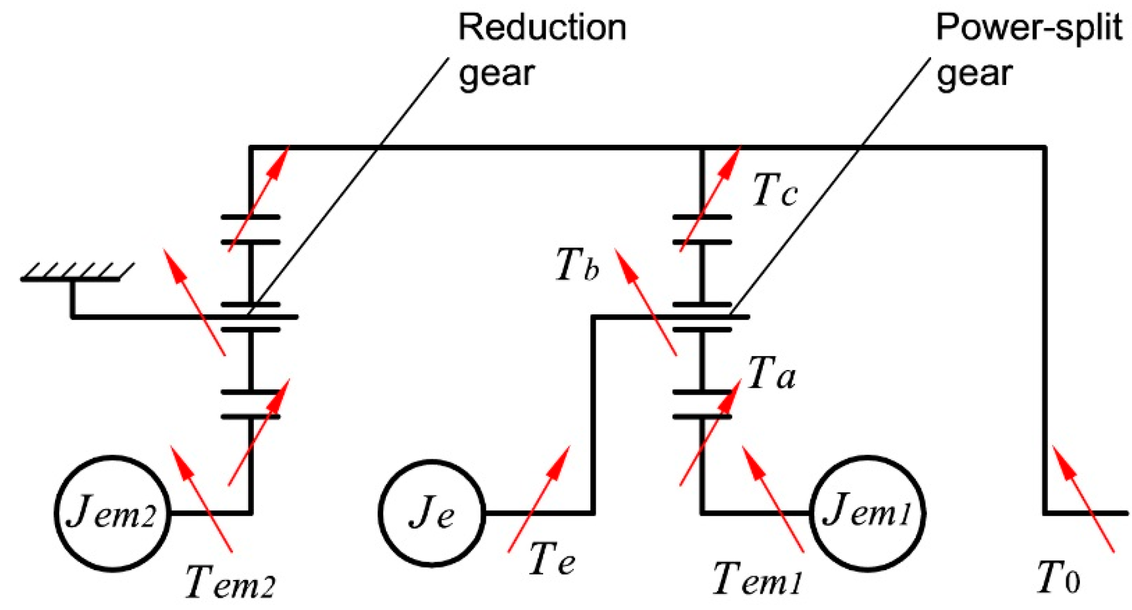
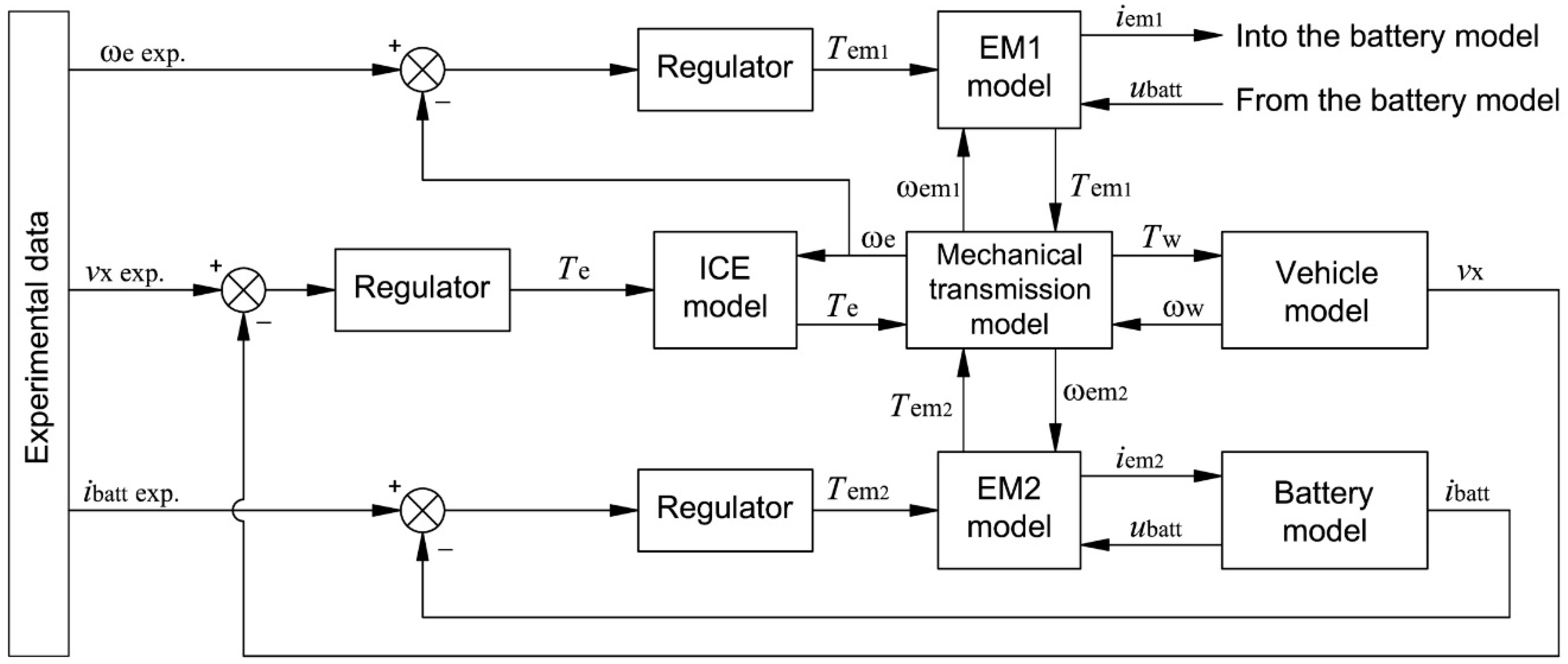
The subject of the second study was a Toyota Prius car equipped with a powertrain called the Toyota Hybrid System (THS), which is often classified as a power-split hybrid transmission [23]. The THS includes an ICE, and two electric machines hereafter called EM1 and EM2. A schematic of the THS is shown in Figure 8. Besides the component designations, it contains the arrows that show direction of the torques exerted by the mentioned driving units, which will be used below for derivation of the mathematical model.

The power-split gear (being an epicyclic gear set) establishes a mechanical connection between all the driving units and the driving wheels. The angular speeds of the input element (the planet carrier) and the output element (the ring gear) of this gear set are mutually independent. This provides two degrees of freedom and, consequently, the ability of stepless regulation of the speed ratio within the mechanical branch of the transmission. The torque ratio of the epicyclic gear set is constant. Stepless regulation of the torque ratio within the THS transmission is provided by the electric branch, which is formed by the EM1 and the EM2. A continuously variable transmission implemented by two said branches allows regulating the ICE speed independently from the vehicle speed. In turn, this allows for the tracking of the engine operating line, minimizing brake specific fuel consumption. ICE speed control is implemented by the EM1, which exerts a balancing torque at the sun gear, operating either as a generator or as a motor—depending on the difference between the speed and torque ratios of the epicyclic gear set. If the former is higher than the latter, the EM1 operates in the generator mode, transmitting a certain part of the power taken from the ICE to the EM2. The latter uses received power to create an additional torque at the transmission output shaft, therefore compensating insufficient torque ratio of the epicyclic gear set. This regime is called the positive split mode and can also be considered as underdrive mode. If the speed ratio is lower than the torque ratio, the EM2, operating in the generation mode, diminishes the output shaft torque and transmits the generated power into the EM1, which operates in the motor mode. As a result, the overdrive (or negative split) regime takes place, in which a certain part of the power provided by the ICE circulates within the transmission. With the ICE and EM1 turned off, the epicyclic gear set is unloaded. ICE’s drag torque prevents its shaft from rotating, which provides disconnection of the ICE from the transmission without using a clutch. In the pure electric mode, the vehicle is driven by the EM2. Cranking of the ICE is performed by the EM1.

Due to presence of two transmission branches and several operating modes (pure electric mode with regenerative braking, positive split, and negative split), the main task in studying the THS powertrain is investigation of the power flows within it. This implies identification of operating points of the powertrain main components, namely, ICE, EM1, EM2, and the traction battery. If direct torque measurements are unavailable, observers should be elaborated for the three driving units.

In this study, the experimental data was obtained from the tests of a Toyota Prius car conducted by ANL and available for using freely under the terms of appropriate referencing (The used experimental data is from the Downloadable Dynamometer Database and was generated at the Advanced Powertrain Research Facility (APRF) at Argonne National Laboratory under the funding and guidance of the U.S. Department of Energy (DOE)). A detailed description of the testing procedure can be found in [24]. The experiments were performed at a chassis dynamometer with simulation of driving cycles. The measured variables relevant for estimation of powertrain operating regimes were vehicle speed, ICE rpm, current, and voltage of the traction battery. Considering the operating principles of the THS system, assignment of the variables to be used by the torque observers was substantiated as follows (other variants are also possible). Since the EM1 controls ICE rpm, the torque of the former should be calculated by a regulator using the experimental ICE rpm signal as the command and its model counterpart as the feedback. In the power-split mode, the ICE power is the major factor controlling the vehicle speed. Thus, the experimental vehicle velocity and its model counterpart were assigned for the ICE torque observer as the command and feedback signals respectively. Similar to the previous case study, the traction EM (i.e., EM2) torque was decided to be calculated using the traction battery current taking into account EM2 efficiency. Figure 9 shows a schematic of the torque observing system elaborated.

The model of vehicle dynamics was derived from the one described in the previous study. Since neither the test conditions nor the structure of the torque observing system implied taking into account the tire slip, the latter was neglected. This allowed the use of a simple kinematic relation between the vehicle velocity and the wheel angular speed. Eliminating the tire forces from the system (3) reduced it to a single equation:

$${\dot{v}}_x=\frac{\left(T_0·u_0\right)/r_w-F_{dyno}-F_{f1}-F_{tr,drag}}{m_v+2{ℐ}_w/r_w^2},$$

(8)

where $T_0$ is the torque at the input shaft of the final drive; $F_{dyno}$ is the steady-speed loading force exerted by a chassis dynamometer, $F_{f1}$ is the rolling resistance of the driving axle tires, and $F_{tr,drag}$ is the drag torque of the mechanical branch of the THS transmission.

The resistance force $F_{dyno}$ was calculated by means of the loading equation specified in the description of the tests. $F_{tr,drag}$ was acquired from the technical report in Reference [25], where it was obtained experimentally as a function of the output shaft angular speed. $F_{f1}$ was evaluated from the make of tires and the energy efficiency class thereof.

The transmission model of the THS was derived from the schematic shown in Figure 8. The following notation is used: $T_e$, $T_{em1}$, and $T_{em2}$ are torques of the ICE, EM1, and EM2 respectively; $T_a$, $T_b$, and $T_c$ are torques at the sun gear, planet carrier, and ring gear respectively; ${ℐ}_e$, ${ℐ}_{em1}$, and ${ℐ}_{em2}$ are inertias of the ICE, EM1, and EM2 respectively. The model equations are based on the torque- and kinematic relations known for the considered type of epicyclic gear set [26]. The output shaft of the transmission is modeled as an element with torsional stiffness and damping, which allows avoiding bulky transformations required for reducing the model to the two-mass system. The resulting system of equations reads:

$$\{\begin{array}{l}{ℐ}_e·{\dot{\omega }}_e=T_e-T_c\left(k+1\right)/k\\ {ℐ}_{em1}·{\dot{\omega }}_{em1}=T_{em1}-T_c/k\\ {\dot{T}}_c=c·\left(-{\omega }_{em2}/u_{red}-{\omega }_0\right)+\gamma ·\left(-{\dot{\omega }}_{em2}/u_{red}-{\dot{\omega }}_0\right)\\ T_0=T_c+(T_{em2}-{ℐ}_{em2}·{\dot{\omega }}_{em2})·u_{red}\\ (-{\omega }_{em2}/u_{red})·k={\omega }_e·\left(k+1\right)-{\omega }_{em1}\\ {\omega }_0·r_w=v_x·u_0\end{array}$$

(9)

where ${\omega }_e$, ${\omega }_{em1}$, and ${\omega }_{em2}$ are shaft angular speeds of the ICE, EM1, and EM2 respectively; k is the quotient of the ring gear teeth number and the sun gear teeth number; c and $\gamma$ are output shaft torsional stiffness and damping coefficient respectively; $u_{red}$ is the speed ratio of the reduction gear placed between the EM2 and the transmission output shaft; ${\omega }_0$ is the angular speed of the transmission output shaft.

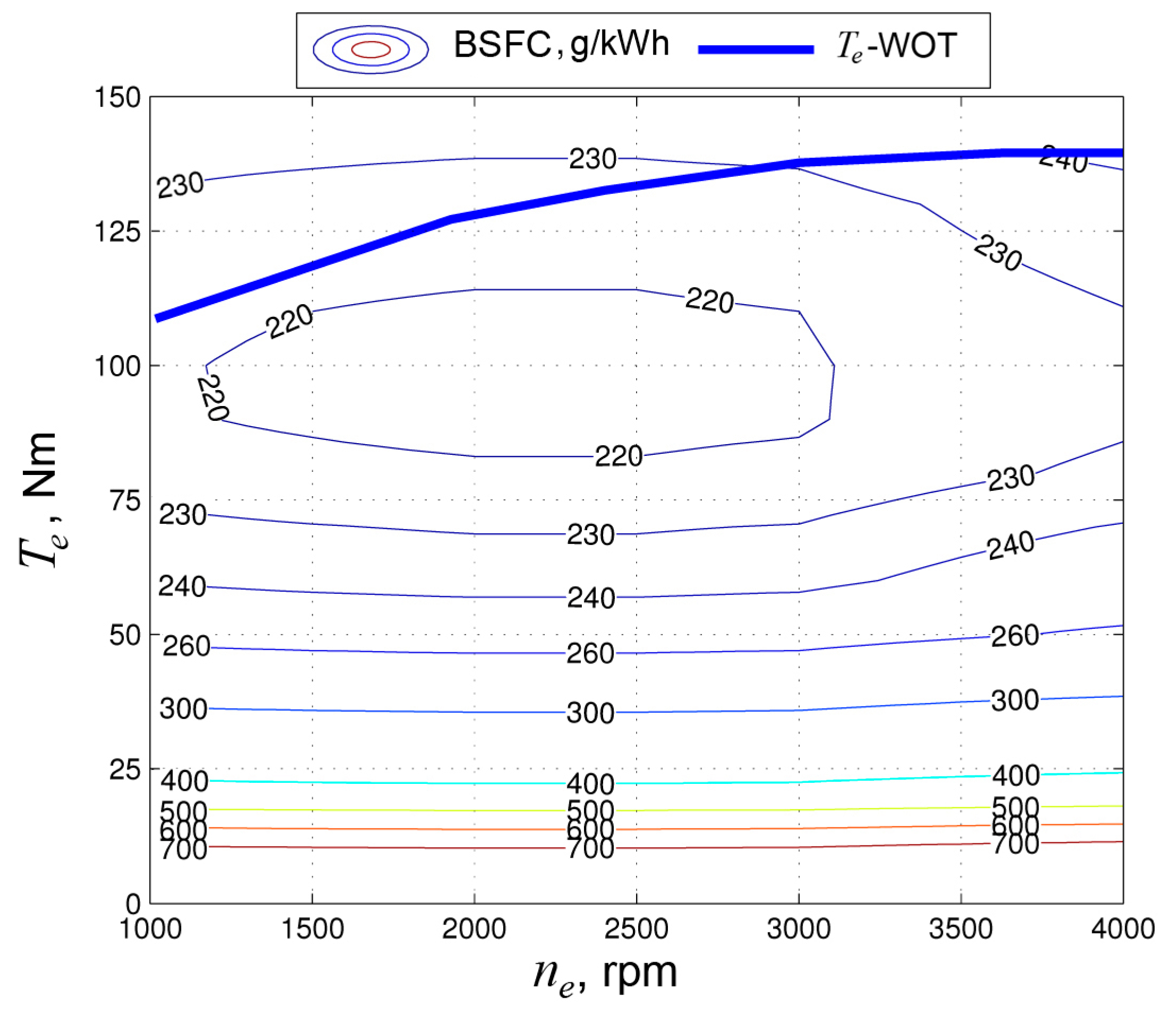
Measured ICE fuel rate and integral fuel consumption can be used to indirectly verify the adequacy of identification of the ICE operating points. Calculation of the fuel consumption implies using a map, which plots the fuel rate against engine rpm and torque. The considered Prius car was equipped with 1.8 L Toyota 2ZR-FXE engine having the maximum power of 73 kW and operating under the Atkinson cycle. The manufacturer provides descriptions of this engine in [27,28]. These materials include the fuel characteristics in the form of map showing the regions of minimum brake specific fuel consumption (BSFC) and the operating line passing through those regions. Using both the map and the data from the chassis dynamometer tests allowed reconstruction of the ICE fuel characteristics. Since the fuel rate characteristics are close to linear in function of both speed and load, these were approximated and used in the ICE model rather than the BSFC. The latter was calculated from the fuel rate approximation and compared to that presented in the manufacturer’s materials, showing a good resemblance to thereof. The calculated BSFC and the wide-open throttle ($T_e$-WOT) characteristics are shown in Figure 10.

The efficiency characteristics of the electric machines of the THS were approximated based on the experimental data from Reference [29]. The traction battery was modelled by an equivalent circuit similar to the one shown in the first case study.

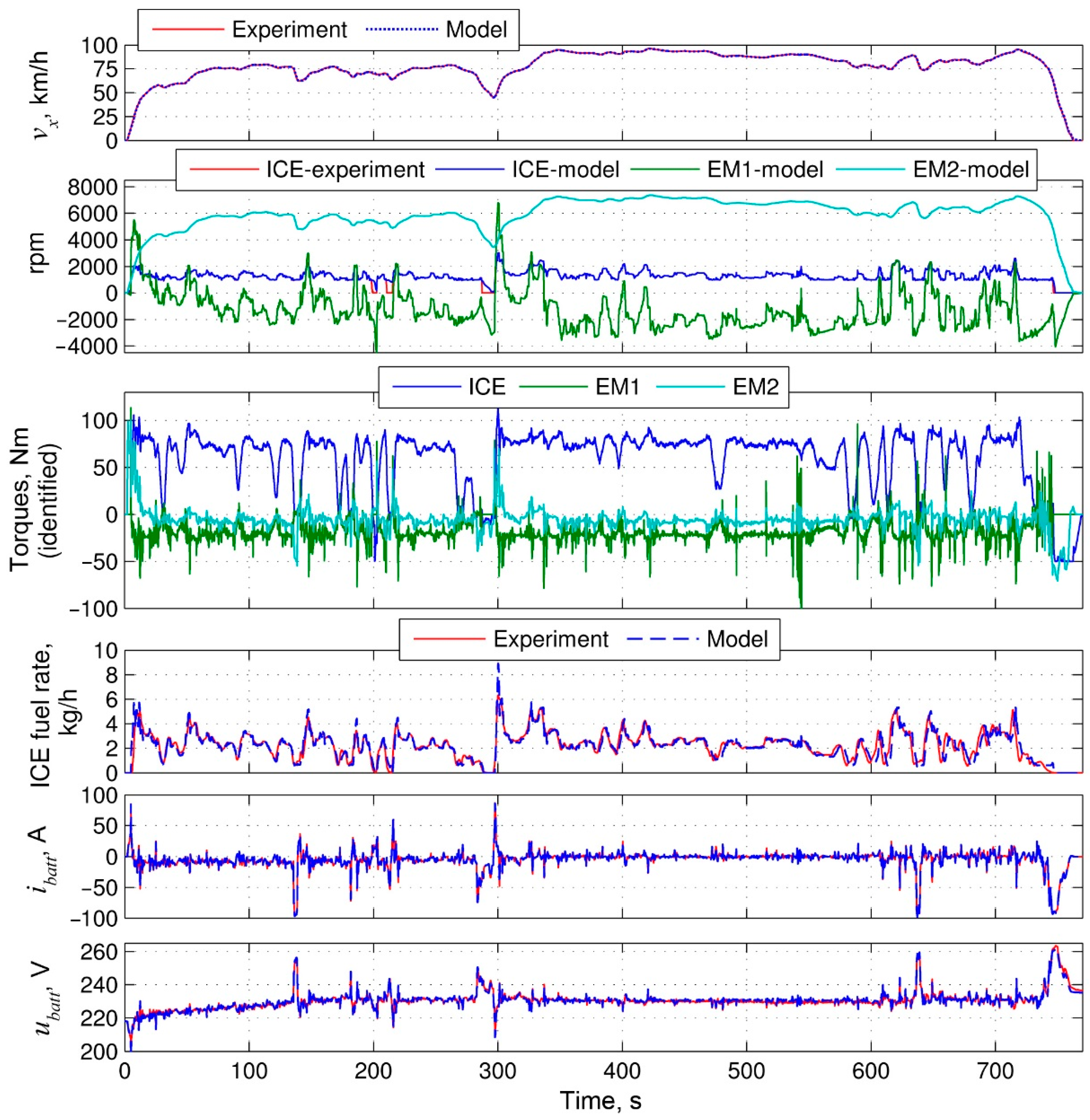
By means of the elaborated model and torque observing system, simulations were conducted replicating the chassis dynamometer experiments. Figure 11 shows both the simulation results and the experimental data obtained in the Highway Fuel Economy Test (HWFET) driving cycle. Note that, for convenience, the EM2 rpm graph is inverted in this figure (when driving forwards, the actual rpm is negative due to the reduction gear placed between the EM2 and the transmission output shaft).

In the driving cycle simulated, the tracking errors constituted 0.2% for the vehicle velocity, 3.25% for the ICE rpm, and 4.9% for the battery current. The bulk of the rpm error was accumulated at the ICE-off periods, where the actual rpm fell to zero, while the modelled rpm did not (note three places between 200 and 300 s where the experimental and simulated rpms do not coincide). However, these periods are not crucial for the study. Neglecting them in the tracking error calculation yields 0.1%. The relative mean square errors of modeling constituted 0.14% for the battery voltage, 8.2% for the ICE fuel rate, and 0.74% for the fuel mass consumed. The fuel consumption obtained in the experiment was 3.94 L/100 km, while the modeling resulted in 3.85 L/100 km.

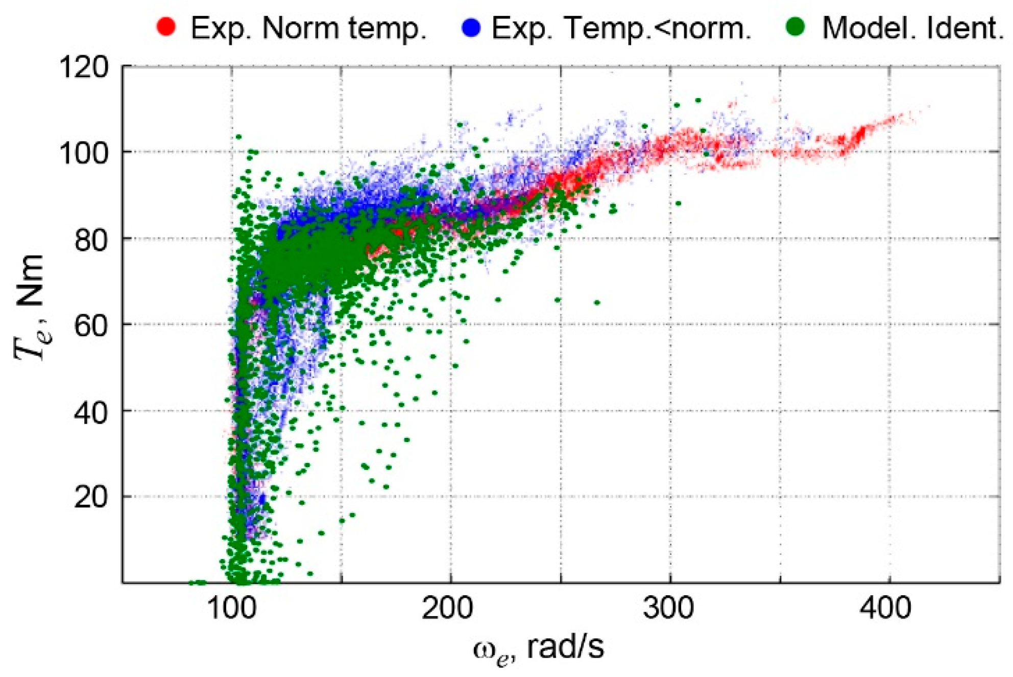
From the simulation results, the ICE operating points (rpm-torque pairs) were extracted and represented graphically in the form of a scattering map. The latter was superimposed with the similar maps presented in other works studying the THS powertrain [3,15,30], in which operating points were identified by means of direct measurements. Figure 12 shows an example of such a comparison using a scattering map (hereafter called “the reference scattering”) obtained by ANL (The reference map is reproduced with a kind permission from the authors of the original source.) [30]. In this diagram, one can see two reference scatterings, of which one was registered with ICE coolant temperature above 92 °C (denoted as “Exp. Norm. temp.”) and other—with the temperature being in range 70–92 °C (denoted as “Exp. Temp < norm”). Comparison of the reference scatterings with the one obtained in this work by means of the torque observation system (denoted as “Model. Ident.”) suggests that the latter provided a correct identification of the unmeasured ICE torque.

5. Conclusions

The lack of torque measurements in tests of electrically driven vehicles or their powertrains can be compensated by employing unknown input observers, which are able to identify non-measured torques using other measured quantities and mathematical modeling.

A form of unknown input observer can be proposed, which is simple, logical, and does not make any changes within the basic structure of the plant’s model. This observer constitutes a feedback control system, which uses the measured signal as the command and its calculated counterpart as the feedback. Compensating difference between these two signals, the regulator calculates a non-measured torque.

Two case studies show that the proposed observer is able to reconstruct unknown operating regimes of powertrain components if there is sufficient number of measured variables, which can be used as commands for regulators.

Indirect and direct verifications of simulation results demonstrate sufficient adequacy of identification provided by the torque observers. These results allow for more thorough and comprehensive studying of powertrains including their operating regimes and efficiency.