Coupling Structural Decomposition Analysis and Sensitivity Analysis to Investigate CO₂ Emission Intensity in China

Abstract

A coupled structural decomposition analysis (SDA) and sensitivity analysis approach is developed to explore the drivers of China’s CO₂ emission intensity at both general and sectoral levels and from both ex-post and ex-ante perspectives. Two steps are involved—structural decomposition and sensitivity analysis. First, the popular factor decomposition method, SDA, is implemented to identify which drivers “have” made the largest contribution to emission intensity changes. Second, an emerging ex-ante approach, sensitivity analysis, is introduced to answer how and to what extent such drivers “will” influence future emission intensity at a sectoral level. Based on China’s input-output tables for 1997–2012, the empirical study provides a hotspot map of China’s energy system. (1) Direct-emission coefficient and technology coefficient are observed as the top two overall drivers. (2) For the former, reducing direct-emission coefficient in an emission-intensity sector (e.g., electricity and heat sectors) by 1% will mitigate China’s total emission intensity by at least 0.05%. (3) For the latter, future emission intensity is super-sensitive to direct transactions in emission-intensity sectors (particularly the chemical industry with elasticities up to 0.82%).

1. Introduction

China’s rapid economic growth has brought forth prosperity; however, such an economic boom has resulted in large environmental costs, such as uncontrolled CO₂ emissions [1,2]. According to statistical data, China’s total CO₂ emissions showed a sharply upward trend from approximately 3206.23 million tons in 2007 to 8506.85 in 2012 at a growth rate above 165%, and China became the world’s largest CO₂ emitter in 2006 [3]. In this context, China has pledged to cut carbon emission intensity (i.e., emissions per unit of gross domestic product (GDP)) by 40–45% by 2020 and 60%–65% by 2030 relative to the level of 2005, hitting the emission reduction peak around 2030 [4,5]. A set of measures have been carried out for a low-carbon economy such as an emissions trading scheme [3]. To design cost-effective mitigation policies, a full understanding of the complicated structure of China’s energy system in terms of the top drivers of China’s emission intensity is an indispensable fundamental task [6]. Therefore, this paper attempts to explore the leading drivers of China’s emission intensity—the most sensitive factors that might cause the highest emissions and should be especially targeted in mitigation policies.

According to the existing literature, the input–output (IO)-based structural decomposition analysis (SDA), a typical ex-post analysis approach, has widely been used to analyze the changes in CO₂ emissions or emission intensity. In particular, based on history data for different periods (e.g., China’s IO tables 1997, 2002, 2007, and 2012 in the case of China), SDA aims to determine the major drivers of emissions or emission intensity, by measuring the relative contribution that a factor “has” made to the total change in emission intensity during the sample period, through two main steps [7,8]. First, we decompose the changes in emissions or emission intensity between two given periods into certain overall factors [9,10]. Second, we estimate the relative contribution of each candidate factor to the total changes, and identify the top leading drivers [11]. Obviously, SDA is a typical ex-post analysis approach, using the IO tables for the sample periods and indicating the drivers that “have” made the largest contributions to the changes of emissions or emission intensity for the sampling periods [12,13]. Based on the IO-based SDA method, consumption volume and production structure were estimated as the primary drivers having changed the CO₂ emission intensity in US the most currently [10,14], while final demand effect and energy intensity for Italy [15,16], and carbonization effect and energy intensity effect for Spanish [17] were also taken into account. In the case of China, the drivers of CO₂ emissions and emission intensity have broadly been studied via different SDA variants, as shown by the recent studies listed in

Table 1. Recent studies on drivers of CO₂ emissions and emissions intensity in China via structural decomposition analysis (SDA).

Authors	Studied System	Leading Driver(s) Identified	Study Period
Zhu et al. [22]	CO2 emissions	Emission intensity; Consumption level	1992–2005
Su & Ang [23]	CO2 emissions	Domestic export; Technology coefficient	2002–2007
Guan et al. [19]	Carbon emission intensity	Emission intensity; Output growth	2002–2009
Su & Ang [18]	Carbon emission intensity	Emission intensity	2007–2010
Li & Wei [24]	CO2 emissions	Emission intensity; Technology coefficient	2002–2010
Xia et al. [25]	CO2 emissions	Emission intensity; Technology effect	2002–2007
Wang et al. [26]	CO2 emissions	Consumption level; Emission intensity	1992–2007
Su & Thomson [27]	CO2 emissions	Emission intensity; Total export effect	2006–2012
Chang & Lahr [28]	CO2 emissions	Emission intensity; Input intensity	2005–2010
Wang & Yang [29]	CO2 emissions	Energy intensity	2000–2010
Nie et al. [20]	CO2 emissions	Technology coefficient; Final demand	1997–2010
Su & Ang [30]	Carbon emission intensity	Emission intensity	2007–2012
Dong et al. [21]	Carbon emission intensity	Energy intensity; Technology coefficient	1992–2012

. From the table, it can be found that emission intensity and technology coefficient were generally identified to be the leading drivers for China’s CO₂ emissions or emission intensity [18,19,20,21].

However, SDA cannot answer the question concerning the identified drivers—how and to what extent they “will” influence future emissions or emission intensity from an ex-ante perspective. Nevertheless, an ex-ante analysis pointing out the hotspots that will lead to massive potential emissions in the future is quite desirable for understanding the energy system and designing the corresponding policies [31]. Furthermore, given that SDA usually decomposes the total changes into several overall factors, it could not probe into more micro-level elements (such as the sectoral coefficients of the target factors) for a specific, practical mitigation policy [32]. Thus, an ex-ante and specific analysis is strongly recommended to help SDA in addressing such tricky problems.

Fortunately, the emerging ex-ante analysis tool, IO-based sensitivity analysis, can be introduced as a perfect complement to SDA for offering an ex-ante and sectoral driver exploration. As a competitive ex-ante analysis, sensitivity analysis can effectively forecast the contribution of a factor to a given target system, by measuring the sensitivity of variations in the target system caused by small changes in the factor [32]. In particular, based on the latest data (e.g., China’s IO table 2012 in the case of China), sensitivity analysis introduces the concept of elasticity to forecast “if” a target coefficient changes (e.g., by 1% in practice) in the near future, and how the associate system (e.g., emission intensity for this study) “will” change accordingly [32,33]. Based on the structure details in IO tables, sensitivity analysis can finely capture the sectoral influential elements in terms of large sensitivity [34,35]. Thus, we specifically introduce a promising such tool, IO-based sensitivity analysis, to extend the ex-post, overall exploration in SDA into an ex-ante, sectoral one.

Some studies have already employed IO-based sensitivity analysis to investigate how and to what extent a sectoral coefficient will influence a target system, as shown by the available works listed in

Table 2. Previous studies using input-output (IO)-based sensitivity analysis.

Authors	Studied Region	Studied System	Studied Coefficient(s)	Data
Hondo et al. [34]	Japan	Emission intensity	Technology coefficient	1990
Tarancón & Del Río [35]	Spain	CO2 emissions	Technology coefficient; Demand coefficient	1995
Tarancón et al. [39]	Spain	CO2 emissions	Technology coefficient	2000
Tarancón et al. [40]	15 Eur. countries	CO2 emissions	Technology coefficient	2003
Tarancón et al. [41]	Spain	Electricity consumption	Technology coefficient	2005
Tarancón & Río [42]	-	CO2 emissions	Technology coefficient	-
Wilting [43]	Netherlands	Greenhouse gas emissions	Technology coefficient	2001
Mattila [36]	Finland	Greenhouse gas emissions	Technology coefficient; DDemand coefficient	2002; 2005
Alcántara et al. [44]	Spain	Electricity consumption	Technology coefficient	2005
Meng et al. [37]	China	Electricity-saving potential	Technology coefficient; DPrice coefficient	2007
Yuan & Zhao [32]	China	CO2 emissions	Technology coefficient	2010
Yan et al. [33]	China	Emission intensity	Technology coefficient	2010
Li et al. [45]	China	Emission intensity	Technology coefficient; DEmissions intensity coefficient	2012

. Interestingly, all the existing related studies focused on energy and environmental systems. However, these works mainly concentrated on technology coefficient (Leontief effect) [32,33,34], demand coefficient [35,36], and price coefficient [37]; in comparison, other even more important coefficients, which have been highlighted in the existing ex-post analyses, such as emission-intensity coefficient [18,26], total export effect [27], input intensity [28], and energy intensity effect [38], were somehow neglected. However, for a systematical exploration of the emission intensity change, a comprehensive sensitivity analysis on at least the leading drivers that have made the greatest contributions to emission intensity change is required. Thus, this paper fills a literature gap by finely coupling sensitivity analysis and SDA, to investigate the main overall drivers of CO₂ emission intensity change that are identified by SDA based on sensitivity analysis. In particular, this study incorporates SDA to determine the major drivers for sensitivity analyses from a systematical perspective; in comparison, the existing related studies pre-determined one or two certain coefficient(s), often omitting some important ones.

Generally, we finely couple SDA and sensitivity analysis, to offer a systematical ex-post, ex-ante, and overall and sectoral analysis for exploring drivers of China’s emission intensity changes. In particular, the proposed approach first implements SDA to reveal the top overall drivers of China’s total emission intensity changes that “have” made the most contribution, and then introduces sensitivity analysis to probe into their sectoral factors to capture the hotspots that “will” lead to massive future emissions in China. To the best of our knowledge, it might be the first attempt to formulate a hybrid SDA and sensitivity analysis approach for exploring the drivers of China’s CO₂ emission intensity. Compared with existing studies, this paper makes major contributions to the literature from the following two perspectives.

(1) By finely combining SDA and sensitivity analysis, this hybrid approach provides a systematical ex-post and ex-ante and overall and sectoral analysis on the drivers of China’s total emission intensity. In particular, it can not only identify the overall drivers that “have” largely impacted China’s total emission intensity via SDA, but also reveal each top driver’s essential sectoral elements that “will” lead to massive future emissions in China via sensitivity analysis.

(2) Four hybrid physical-monetary energy IO tables in China for 1997, 2002, 2007, and 2012 are compiled, to not only capture the long-term trends for 1997–2012 in the ex-post analysis, but also conduct the ex-ante analysis based on the most updated data for 2012. In particular, a map of hotspots in China’s energy system leading to the highest potential emissions can be drafted for facilitating the design and adjustment of specific, target-mitigation policies.

The rest of the paper is organized as follows. Section 2 describes the formulation process of the proposed methodology. The empirical results are reported and discussed in Section 3. Section 4 concludes the paper and outlines major directions of future research.

2. Methodology

For a clear discussion, the general framework of the proposed methodology is presented in Section 2.1. Section 2.2 gives a brief introduction to the standard IO model, based on which the methodology is built. Section 2.3 and Section 2.4 describe the two main steps of the methodology, respectively.

2.1. General Framework

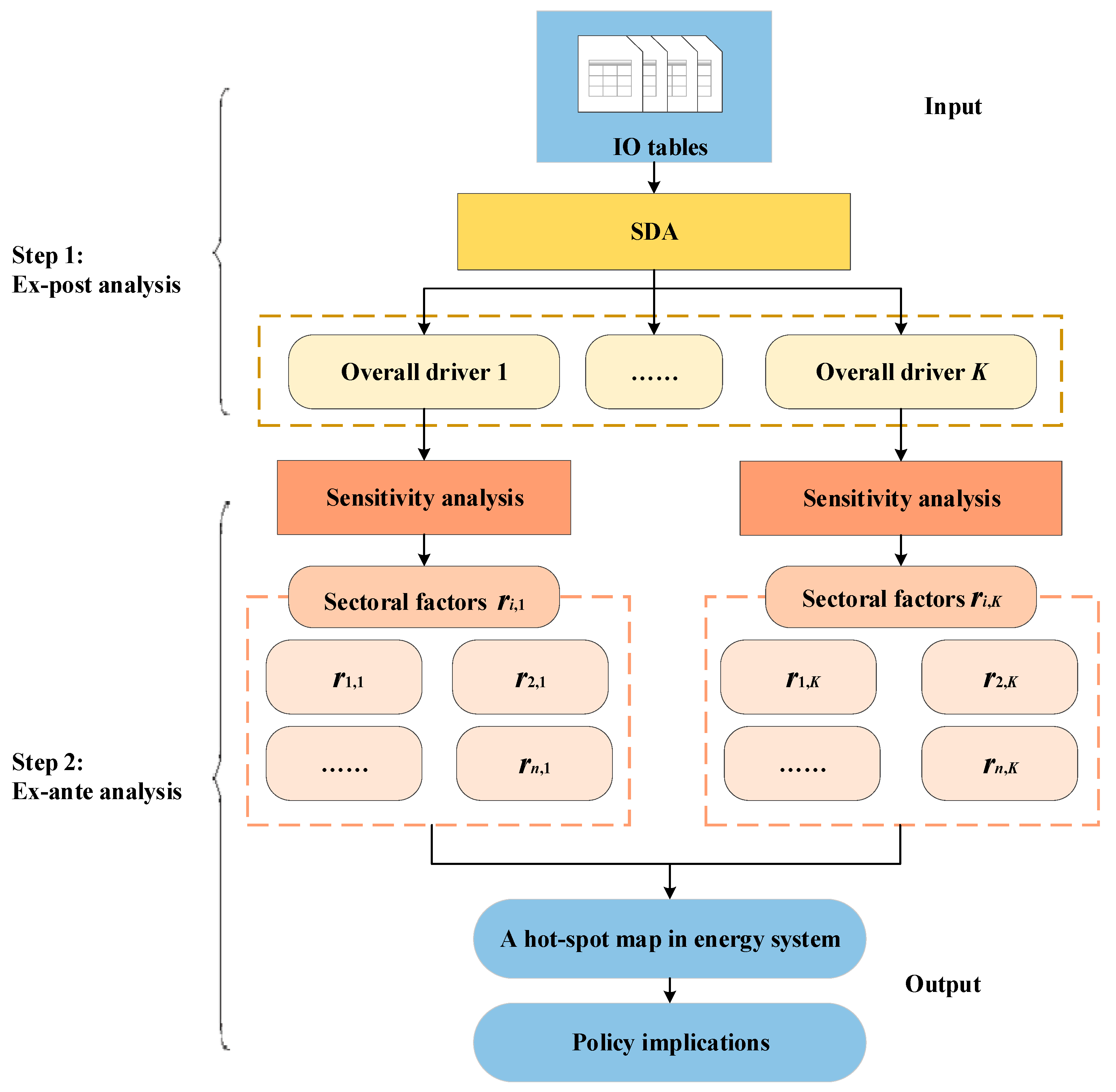
In this section, a hybrid SDA and sensitivity analysis approach is formulated not only to (1) explore overall drivers that have largely changed CO₂ emission intensity via SDA, but also to (2) investigate each top driver to identify its key sectoral elements leading to potential massive future emissions via sensitivity analysis. Accordingly, two major steps, structural decomposition analysis and sensitivity analysis, are included in the proposed model, as per the framework illustrated in Figure 1.

Step 1: Ex-post analysis via SDA

The prevailing factor decomposition, SDA, is implemented to decompose CO₂ emission intensity into four overall drivers: direct-emission coefficient (C), technology coefficient (B), final demands structure by product (D), and final demands by category (F). Then, the two-polar decomposition method is introduced to measure the contribution of each driver to the changes in total emission intensity, to identify the top drivers that have made up the largest changes during the sampling periods.

Step 2: Ex-ante analysis via sensitivity analysis

The top leading drivers are further analyzed via a promising ex-ante analysis method, sensitivity analysis, to reveal how and to what extent they will influence the emission intensity. In particular, a map of hotspots in the energy system, i.e., the influential sectoral factors r_i,j (i = 1,…, n; j = 1,…, K) which will lead to the highest growth in emissions, can be provided, where r_i,j is the ith essential element of the jth major driver. With the above valuable information, insightful suggestions can be deduced for the design and adjustment of specific, targeted mitigation policies.

2.2. Input-Output Model

The proposed hybrid approach is based on the IO model (or IO table) as per the database. Therefore, a hybrid physical–monetary energy IO model is compiled, including a basic IO model in monetary units and an emissions IO model in physical units.

2.2.1. Basic IO Model

The IO model is developed from an inter-industry transaction table to capture the flows of products between economic sectors (or industries) in a macro-economic system [46,47]. It is assumed that a total of n interactive economic sectors conduct production activities and provide total outputs (in term of goods and services) of the whole economic system, which meets total final demand covering 6 categories here: household consumption, government consumption, fixed capital formation, changes in inventories, net exports, and others.

In a monetary IO model, the output of sector i is computed based on the following balance equation, while the intermediate input/demand ($z_{i,j}$), final demand ($y_i$) and output ($x_i$) are represented in the monetary unit [48,49]:

$${\displaystyle \sum _{j=1}^n{z}_{i,j}}+y_i=x_i$$

(1)

where $z_{i,j}$ represents the intermediate input from sector i to sector j, $y_i$ is the final demand of sector i, and $x_i$ is the total output of sector i. The technical coefficient $a_{i,j}$ can be defined as the direct consumption of sector j by unit input of sector i [50].

$$a_{i,j}=z_{i,j}/x_j$$

(2)

where $x_j$ is the total input of sector j. The technical coefficients $a_{i,j}$ for different sectors j = 1,.., n constitute the economy’s direct consumption coefficient matrix of the monetary table $A= [a_{i,j}]$. The consumption of sector i can be obtained based on the inverse Leontief matrix (or matrix of total requirement coefficient), i.e., $B={\left(I-A\right)}^{-1}=\left[b_{i,q}\right]$ [51].

$$x_i={\displaystyle \sum _{q=1}^n{b}_{i,q}}\cdot y_q$$

(3)

where $b_{i,q}$ is the qth elements in the ith row of the inverse Leontief matrix B. The final demand structure by product can be described as [52]

$$D=[d_{i,t}]=[\raisebox{1ex}{$y_{i,t}$}\!\left/ \!\raisebox{-1ex}{$f_t$}\right.]$$

(4)

where the element $d_{i,t}$ represents the share of sector i in the final demand of category t and ${\displaystyle \sum _i^n{d}_{i,t}}=1$, $f_t$ is the final demand of category t, and $y_{i,t}$ is the final demand of category t for the product by sector i [53]. Therefore, the final demand can be expressed as

$$Y=DF$$

(5)

where $F=[f_t]=[{\displaystyle \sum _i^n{y}_{i,t}}]$ is the column vector of final demands by category. The column vector of total output X can be expressed as [54].

$$X=BDF$$

(6)

2.2.2. Emissions in IO Model

The energy-related CO₂ emissions are calculated based on the direct consumption of the energy, via the IPCC reference approach [55]. The corresponding data are derived from China’s energy balance tables from 1997, 2002, 2007, and 2012, which were compiled by the China National Bureau of Statistics. Notably, this study focuses on the CO₂ emissions from production (i.e., production-based emissions), whereas the CO₂ emissions from residential energy consumption (which is also available in China’s energy balance tables) are not considered [56]. Therefore, from the production-based perspective, sectoral emissions were estimated for each sector from the five types of energy that could possibly be used (coal (covering raw coal, cleaned coal, and other washed coal), natural gas, coke, finished oil (covering diesel oil, gasoline, kerosene, and fuel oil), and liquefied petroleum gas) [28].

Let $e_{k,i}$ be the CO₂ emissions from the direct consumption of energy k during the production by sector i (that are calculated based on the data from China’s energy balance tables), which is expressed in physical units, such that the CO₂ emissions from sector i can be computed by $e_i={\displaystyle {\sum }_{k=1}^m{e}_{k,i}}$ and the associated direct-emission coefficient $C=[c_i]\in R^{1\times n}$—the CO₂ emissions from the production per unit of sectoral output—can be defined as [57]

$$C=[c_i]=[\frac{e_i}{x_i}]=[\frac{{\displaystyle \sum _{k=1}^m{e}_{k,i}}}{x_i}]=[{\displaystyle \sum _{k=1}^m{c}_{k,i}}]$$

(7)

where x_i is the output of sector i (derived from China’s monetary IO tables). Accordingly, the total production-based CO₂ emissions across different sectors (in physical unit) can be calculated in terms of the product of direct-emission coefficient C and the output $X=[x_i]\in R^{n\times 1}$ [58]:

$$TE=\mathsf{\mu }CX=\mathsf{\mu }CBDF$$

(8)

where $\mathsf{\mu }$ represents a 1 × m summation row vector. GDP can be expressed as

$$GDP=\lambda F$$

(9)

where $\lambda$ is a 1 × n summation row vector. Finally, the total CO₂ emission intensity China’s total emission intensity (CEI) can be defined as

$$CEI=TE/GDP=\mathsf{\mu }CBDF/\lambda F$$

(10)

where the emission intensity CEI is then in units of kg CO₂/yuan [59].

2.3. Structural Decomposition Analysis

A series of economic factors (e.g., economic growth, economic structure, and infrastructure investment) and technologic factors (particularly the energy-related technology development) simultaneously affect the total emission intensity. To identify the top leading drivers among them, the SDA method has widely been considered to be one of the most useful tools, measuring the relative contribution of each candidate factor to the changes in total emission intensity [22,60,61].

The changes of total emission intensity CEI in Equation (10) between a reference time (as marked with subscript 1) and a base time (with subscript 0) can be defined in the form of a ratio.

$$CE{I}_1/CE{I}_0=\frac{\mathsf{\mu }{C}_1{B}_1{D}_1{F}_1}{\mathsf{\mu }{C}_0{B}_0{D}_0{F}_0}\times \frac{\lambda F_0}{\lambda F_1}$$

(11)

According to Equation (11), the changes in total emission intensity can be decomposed into four overall factors: (1) direct-emission coefficient C, (2) technology coefficient B, (3) final demands structure by product D, and (4) final demands by category F. The two-polar decomposition method is introduced to conduct the estimation, i.e., decomposing Equation (11) at the base time and reference time respectively and then averaging the two polar values as the results [59,62]. From the base time 0, the total emission intensity in Equation (11) can be decomposed into

$$CE{I}_1/CE{I}_0=\frac{\mathsf{\mu }{C}_1{{\rm B}}_0{D}_0{F}_0}{\mathsf{\mu }{C}_0{B}_0{D}_0{F}_0}\times \frac{\mathsf{\mu }{C}_1{B}_1{D}_0{F}_0}{\mathsf{\mu }{C}_1{B}_0{D}_0{F}_0}\times \frac{\mathsf{\mu }{C}_1{B}_1{D}_1{F}_0}{\mathsf{\mu }{C}_1{B}_1{D}_0{F}_0}\times \frac{\mathsf{\mu }{C}_1{B}_1{D}_1{F}_1}{\mathsf{\mu }{C}_1{B}_1{D}_1{F}_0}\times \frac{\lambda F_0}{\lambda F_1}$$

(12)

From the reference time 1, it can be

$$CE{I}_1/CE{I}_0=\frac{\mathsf{\mu }{C}_1{B}_1{D}_1{F}_1}{\mathsf{\mu }{C}_0{B}_1{D}_1{F}_1}\times \frac{\mathsf{\mu }{C}_0{B}_1{D}_1{F}_1}{\mathsf{\mu }{C}_0{B}_0{D}_1{F}_1}\times \frac{\mathsf{\mu }{C}_0{B}_0{D}_1{F}_1}{\mathsf{\mu }{C}_0{B}_0{D}_0{F}_1}\times \frac{\mathsf{\mu }{C}_0{B}_0{D}_0{F}_1}{\mathsf{\mu }{C}_0{B}_0{D}_0{F}_0}\times \frac{\lambda F_0}{\lambda F_1}$$

(13)

Finally, the decomposition results are computed by averaging the two polar results in Equations (12) and (13).

$$CE{I}_1/CE{I}_0=\Delta C\times \Delta B\times \Delta D\times \Delta F$$

(14)

$$\Delta C=\sqrt{\frac{\mathsf{\mu }{C}_1{B}_0{D}_0{F}_0}{\mathsf{\mu }{C}_0{B}_0{D}_0{F}_0}\times \frac{\mathsf{\mu }{C}_1{B}_1{D}_1{F}_1}{\mathsf{\mu }{C}_0{B}_1{D}_1{F}_1}}$$

(15)

$$\Delta B=\sqrt{\frac{\mathsf{\mu }{C}_1{B}_1{D}_0{F}_0}{\mathsf{\mu }{C}_1{B}_0{D}_0{F}_0}\times \frac{\mathsf{\mu }{C}_0{B}_1{D}_1{F}_1}{\mathsf{\mu }{C}_0{B}_0{D}_1{F}_1}}$$

(16)

$$\Delta D=\sqrt{\frac{\mathsf{\mu }{C}_1{B}_1{D}_1{F}_0}{\mathsf{\mu }{C}_1{B}_1{D}_0{F}_0}\times \frac{\mathsf{\mu }{C}_0{B}_0{D}_1{F}_1}{\mathsf{\mu }{C}_0{B}_0{D}_0{F}_1}}$$

(17)

$$\Delta F=\sqrt{\frac{\mathsf{\mu }{C}_1{B}_1{D}_1{F}_1}{\mathsf{\mu }{C}_1{B}_1{D}_1{F}_0}\times \frac{\lambda F_0}{\lambda F_1}\times \frac{\mathsf{\mu }{C}_0{B}_0{D}_0{F}_1}{\mathsf{\mu }{C}_0{B}_0{D}_0{F}_0}\times \frac{\lambda F_0}{\lambda F_1}}$$

(18)

where the coefficients $\Delta C$, $\Delta B$, $\Delta D$, and $\Delta F$ in Equations (15)–(18) are the changes of factors C, B, D, and F, respectively.

2.4. Sensitivity Analysis

Because SDA mainly focuses on overall, ex-post analyses, this work especially introduces sensitivity analysis as a perfect complement to SDA to provide a specific, ex-ante analysis. In particular, the sensitivity analysis in this study was proposed by Tarancón in 2007, which is based on the IO model to identify the most relevant factors in terms of environmental indicators at sectoral level [35]. In sensitivity analysis, an indicator, namely coefficient elasticity, was developed to assess which transactions between economic sectors can be expected to bear a greater impact on CO₂ emissions in sectors [32,33].

Sensitivity analysis can provide a map of hotspots in the energy system, in terms of influential specific elements, i.e., r_i,j (i = 1,…, n; j = 1,…, K) where r_i,j is the ith essential sectoral element of the jth major driver [32]. In this study, an elasticity indicator is introduced to measure the sensitivity of total emission intensity to the target coefficient r_i,j, i.e., the extent to which a change in r_i,j influences the total emission intensity [33].

For a clear understanding, a general form of sensitivity analysis on any target driver is first formulated in Section 2.4.1. Taking for example direct-emission coefficient and technology coefficient—two leading drivers according to previous studies—the corresponding variants are developed in Section 2.4.2 and Section 2.4.3, respectively; the ones for other drivers follow a similar form.

2.4.1. General Form

At a sector level, the sectoral emission intensity $CE{I}_i$ can be defined as the emissions from the production per unit of value added in sector i [21,33].

$$CE{I}_i=e_i/V{A}_i$$

(19)

where $CE{I}_i$ represents the emission intensity of sector i, and $V{A}_i$ is the value added of sector i. Accordingly, the total emission intensity for sectors CEI in Equation (10), i.e., the total CO₂ emissions from the production per unit of GDP, can be expressed as [32]

$$CEI=\frac{TE}{GDP}=\frac{{\displaystyle \sum _{i=1}^n{e}_i}}{{\displaystyle \sum _{i=1}^{n}V{A}_i}}$$

(20)

where $TE={\displaystyle \sum _{i=1}^n{e}_i}$ indicates the total CO₂ emissions from the production across all the sectors [33].

Based on the elasticity indicator, the sensitivity of emission intensity to the target coefficient r_i,j, i.e., the extent to which a change in r_i,j influences emission intensity for sector m, can be defined as

$${\epsilon }_{CE{I}_m,r_{i,j}}=\frac{\Delta CE{I}_m/CE{I}_m}{\Delta r_{i,j}/r_{i,j}}$$

(21)

where r_i,j represents the specific element of the jth driver in sector i, ${\epsilon }_{CE{I}_m,r_{i,j}}$ is the elasticity index reflecting the sensitivity of emission intensity of sector m to the coefficient r_i,j, $\Delta r_{i,j}$ is the change in r_i,j, and $\Delta CE{I}_m$ represents the change of emission intensity in sector m impacted by the change in r_i,j (i.e., $\Delta r_{i,j}$). In practice, a given small variation of the related coefficient, e.g., 1%, is set to calculate such a sensitivity, i.e., $\Delta r_{i,j}=0.01r_{i,j}$.

Similarly, the effect of the change $\Delta r_{i,j}$ on the total emission intensity from all sectors is expressed as

$${\epsilon }_{CEI,r_{i,j}}=\frac{\Delta CEI/CEI}{\Delta r_{i,j}/r_{i,j}}$$

(22)

where ${\epsilon }_{CEI,r_{i,j}}$ is the elasticity index reflecting the sensitivity of total emission intensity to the coefficient r_i,j. Given that sectoral emission intensity $CE{I}_i$ closely relates to the total emission intensity CEI according to Equations (19) and (20), the sectoral effect ${\epsilon }_{CE{I}_m,r_{i,j}}$ due to a coefficient change $\Delta r_{i,j}$ might largely impact the total effect ${\epsilon }_{CEI,r_{i,j}}$.

2.4.2. Sensitivity Analysis on Direct-Emission Coefficient

The direct-emission coefficient C has consistently been identified as the top key driver of China’s total emission intensity change in the existing studies. According to Equation (7), the direct-emission coefficient for sector i-c_i, the ith sectoral element of the factor C, represents the emissions per unit of output value in sector i. Obviously, a larger value of direct-emission coefficient corresponds to a higher emission-intensity sector.

Based on the general form in Equation (22), the elasticity index ${\epsilon }_{CEI,c_i}$ can be estimated by

$${\epsilon }_{CEI,c_i}=\frac{\Delta CEI/CEI}{\Delta c_i/c_i}=\left[\Delta \left(\frac{{\displaystyle \sum _{i=1}^n{c}_i\cdot x_i}}{{\displaystyle \sum _{i=1}^{n}V{A}_i}}\right)/\frac{{\displaystyle \sum _{i=1}^n{c}_i\cdot x_i}}{{\displaystyle \sum _{i=1}^{n}V{A}_i}}\right]\cdot \frac{c_i}{\Delta c_i}=\frac{\Delta {\displaystyle \sum _{i=1}^n{c}_i\cdot x_i}}{{\displaystyle \sum _{i=1}^n{c}_i\cdot x_i}}\cdot \frac{c_i}{\Delta c_i}$$

(23)

The ${\displaystyle \sum _{i=1}^{n}V{A}_i}$ is the added value (stemming from the 3th quadrant of IO table), without the effect of sectoral direct-emission coefficients change $\Delta c_i$. Obviously, the elasticity index ${\epsilon }_{CEI,c_i}$ for ith sectoral element of the driver C is only dependent on the direct-emission coefficient of sector i(c_i). The sensitivity analysis on direct-emission coefficient C can effectively identify the key sectors, whose changes of sectoral direct-emission coefficients $\Delta c_i$ severely impact the total emission intensity CEI in terms of high ${\epsilon }_{CEI,c_i}$.

2.4.3. Sensitivity Analysis on Technology Coefficient

According to the previous studies, the technology coefficient B is also a key driver of China’s total emission intensity change. The sensitivity analysis on B has recently aroused an increasing interest in the research field of CO₂ emissions analysis [32,33] to reveal the essential linkages between sectors which will lead to the highest growth of CO₂ emissions.

By introducing Equations (3) and (7), Equation (19) can be rewritten as

$$CE{I}_i=\frac{c_i\cdot {\displaystyle \sum _{q=1}^n{b}_{i,q}}\cdot y_q}{V{A}_i}$$

(24)

Accordingly, the changes in emission intensity of sector m ($\Delta CE{I}_m$) caused by the variation of sectoral technology coefficient b_m,q (i.e., $\Delta b_{m,q}$) can be defined as

$$\Delta CE{I}_m=\frac{c_m\cdot {\displaystyle \sum _{q=1}^n\Delta b_{m,q}}\cdot y_q}{V{A}_m}$$

(25)

where $\Delta b_{m,q}$ represents the variation of the technology coefficient $b_{m,q}$. $\Delta CE{I}_m$ represents the change of emission intensity in sector m impacting by the change in $b_{m,q}$ (i.e., $\Delta b_{m,q}$). The added value of sector i (i.e., $V{A}_i$) is constant despite the change in $b_{m,q}$. Therefore, the change of emission intensity in sector m ($\Delta CE{I}_m$) here is only dependent on the $\Delta b_{m,q}$, as shown in Equation (25).

Given that B = (I − A)⁻¹ = [b_m,q], $\Delta b_{m,q}$ is actually the changes in technical coefficient $\Delta a_{i,k}$ corresponding to the technological mix of sector k. According to the core Sherman–Morrison formula of error-propagation theory [63], a change in the technological mix of sector k (i.e., $\Delta a_{i,k}$) would affect the quality in emission intensity of sector m (i.e., $\Delta CE{I}_m$), through the changes experienced by the elements of the inverse Leontief matrix corresponding to row m [63]:

$$\Delta b_{m,q}=\frac{b_{m,i}\cdot b_{k,q}\cdot \Delta a_{i,k}}{1-b_{k,i}\cdot \Delta a_{i,k}}$$

(26)

where $\Delta a_{i,k}$ is the changes of technology coefficient a_i,k. By introducing Equation (26) to Equation (25) for the relationship between $\Delta b_{m,q}$ and $\Delta CE{I}_m$, the relationship running from $\Delta a_{i,k}$ (for sector k) to $\Delta CE{I}_m$ (for sector m) can be mathematically described as

$$\Delta CE{I}_m=\frac{c_m}{V{A}_m}\cdot {\displaystyle \sum _{q=1}^n\frac{b_{m,i}\cdot b_{k,q}\cdot \Delta a_{i,k}}{1-b_{k,i}\cdot \Delta a_{i,k}}}\cdot y_q=\frac{c_m}{V{A}_m}\cdot \frac{b_{m,i}\cdot x_k\cdot \Delta a_{i,k}}{1-b_{k,i}\cdot \Delta a_{i,k}}$$

(27)

Based on the elasticity indicator, the extent to which the technology change $\Delta a_{i,k}$ influences the sectoral emission intensity can be estimated by [33]

$${\epsilon }_{CE{I}_m,a_{i,k}}=\frac{\Delta CE{I}_m/CE{I}_m}{\Delta a_{i,k}/a_{i,k}}=\frac{b_{m,i}\cdot a_{i,k}}{1-b_{k,i}\cdot \Delta a_{i,k}}\cdot \frac{x_k}{x_m}$$

(28)

where the elasticity index ${\epsilon }_{CE{I}_m,a_{i,k}}$ represents the extent to which the change in technology coefficient $\Delta a_{i,k}$ of sector k influences the emission intensity of sector m. Obviously, the former factor in Equation (28) is totally determined by the technology coefficient $a_{i,k}$; in contrast, the latter factor $x_k/x_m$ corresponds to the output of sector k with respect to the that of sector m. The output of sector k (i.e., $x_k={\displaystyle \sum _{q=1}^n{b}_{k,q}}\cdot y_q$) is affected by technical coefficient (${\displaystyle \sum _{q=1}^n{b}_{k,q}}$) and final demand ($y_q$). Accordingly, the elasticity ${\epsilon }_{CE{I}_m,a_{i,k}}$ measures not only the effect of technological changes $\Delta a_{i,k}$ of sector k on the emission intensity of sector m, but also the effect of the economic structure of final demand. Therefore, ${\epsilon }_{CE{I}_m,a_{i,k}}$ can be termed as the “structure-relevant” technical coefficient elasticity (TCE). To independently investigate how the technical change influences the sectoral emission intensity, we employ a uniform vector of final demand, i.e., $y_q=1$ for $\forall q$. Thus, the “technology-relevant” TCE, which only considers the effect of technological changes, can be obtained as follows:

$${\epsilon }_{CE{I}_m{}_{,}{a}_{i,k}}^{*}=\frac{b_{m,i}\cdot a_{i,k}}{1-b_{k,i}\cdot \Delta a_{i,k}}\cdot \frac{{\displaystyle \sum _{q=1}^n{b}_{k,q}}}{{\displaystyle \sum _{q=1}^n{b}_{m,q}}}$$

(29)

where ${\epsilon }_{CE{I}_m{}_{,}{a}_{i,k}}^{*}$ is the corresponding “technology-relevant” TCE of ${\epsilon }_{CE{I}_m,a_{i,k}}$, without considering the impact of the final demand structure. Notably, the assumption of setting the final demand vector to a uniform vector in calculating the “structure-relevant” TCE ${\epsilon }_{CE{I}_m{}_{,}{a}_{i,k}}^{*}$ might be far away from the real world. Therefore, the results analyses in Section 3.5 will be mainly based on the elasticity ${\epsilon }_{CE{I}_m,a_{i,k}}$ (without this assumption), rather than ${\epsilon }_{CE{I}_m{}_{,}{a}_{i,k}}^{*}$ (with this assumption).

However, the elasticity ${\epsilon }_{CE{I}_m{}_{,}{a}_{i,k}}^{*}$ has widely been employed in the existing literature (e.g., [32,33]), in order to reveal the insightful findings—a general direction of designing mitigation policies, i.e., whether to prioritize addressing the technology-relevant coefficients for production (if ${\epsilon }_{CE{I}_m{}_{,}{a}_{i,k}}\ll {\epsilon }_{CE{I}_m{}_{,}{a}_{i,k}}^{*}$) or the structure-relevant ones for final demand (if ${\epsilon }_{CE{I}_m{}_{,}{a}_{i,k}}\gg {\epsilon }_{CE{I}_m{}_{,}{a}_{i,k}}^{*}$).

Through sensitivity analysis on technology coefficient B, the essential sector linkages, whose changes in sectoral technology coefficient $\Delta a_{i,k}$ severely impact the emission intensity in terms of high ${\epsilon }_{CE{I}_m,a_{i,k}}$ and ${\epsilon }_{CE{I}_m{}_{,}{a}_{i,k}}^{*}$ values, can be identified.

3. Empirical Study

An empirical study on China is conducted for illustration and verification. First, Section 3.1 presents the data descriptions. Second, the CO₂ emissions and emission intensity for 1997–2012 are estimated via the IO model, as per the results reported in Section 3.2. Third, the proposed hybrid approach is employed to explore the top overall drivers (discussed in Section 3.3) and key sectoral factors (Section 3.4 and Section 3.5) in changing China’s total emission intensity. Third, Section 3.6 concludes the major findings and provides the corresponding policy measures.

3.1. Data Descriptions

This paper investigates the leading drivers of China’s total emission intensity change via a hybrid SDA and sensitivity analysis approach, which is based on the IO tables as the database. Therefore, four pairs of hybrid physical-monetary energy IO tables for the years 1997, 2002, 2007, and 2012 are compiled, covering two types of data—time-series IO tables (in monetary units) and the corresponding emissions data (in physical units). For the monetary data, China’s IO tables for 1997, 2002, 2007, and 2012 are obtained from the China Statistical Yearbook, which is compiled by the National Bureau of Statistics of China. According to China’s standard industrial classification system, this study classifies China’s industries into 21 sectors (indicating the i and j in Equation (1)), as listed in

Table 3. Sectors in China’s input-output model.

Abbr.	Sector	Abbr.	Sector
n1	Coal mining and dressing	n12	Chemical industry
n2	Extraction of petroleum and natural gas	n13	Non-metallic mineral products
n3	Processing of petroleum, coking, and nuclear fuel	n14	Smelting and pressing of metals
n4	Production and supply of electric power and heat	n15	Manufacture of metal products
n5	Production and supply of gases	n16	Manufacture of general equipment
n6	Agriculture, forestry, animal fishery	n17	Production and supply of water
n7	Ores mining and dressing	n18	Construction
n8	Manufacture of foods, beverages, and tobacco	n19	Transport, storage, and post
n9	Manufacture of textile, leather, fur, feather, and other fiber products	n20	Wholesale and retail trades, hotel, and catering service
n10	Processing and manufacture of timber and furniture	n21	Other services
n11	Manufacture of paper, printing, cultural, and educational articles

.

For the physical data, energy consumption data (in standard coal equivalent) are derived from the China Energy Statistical Yearbook. In particular, the energy balance tables refer to the summation of the direct energy consumptions by all the sectors and energy losses. In this paper, we collected seven main types of energy, i.e., coal (covering raw coal, cleaned coal, and other washed coal), natural gas, coke, finished oil (covering diesel oil, gasoline, kerosene, and fuel oil), liquefied petroleum gas, and heat, and electricity. Generally, most CO₂ emissions are caused by the combustion of fossil fuels, in which CO₂ emissions in heat and electricity generation should be allocated to the heat and electricity sector and not to heat and electricity use [25]. To avoid double calculation, these energies are aggregated into 5 forms (indicating the k in Equation (7)), without considering the heat, and electricity consumption. In this paper, the CO₂ emissions are generated by the consumption of five types of energy in the production process of 21 sectors. Therefore, the production-based CO₂ emissions (in 10,000 tons of standard coal equivalent) from fuel combustion are calculated, via the IPCC reference approach [55]. To avoid the potential impact of price changes, monetary tables are all converted to 2002 constant price (in RMB, 10,000 Yuan) by using sectoral price indexes [64]. In particular, the price indexes for the industrial sectors (n1–n5 and n7–n17), agriculture sector (n6), transportation sector (n19), and services sector (n20 and n21) are obtained from the corresponding sectoral price indices tables in China Statistical Yearbooks, while those for the construction sector (n18) are presented by the investment in fixed assets according to the China Statistical Abstract [65,66].

3.2. CO₂ Emissions and Emission Intensity

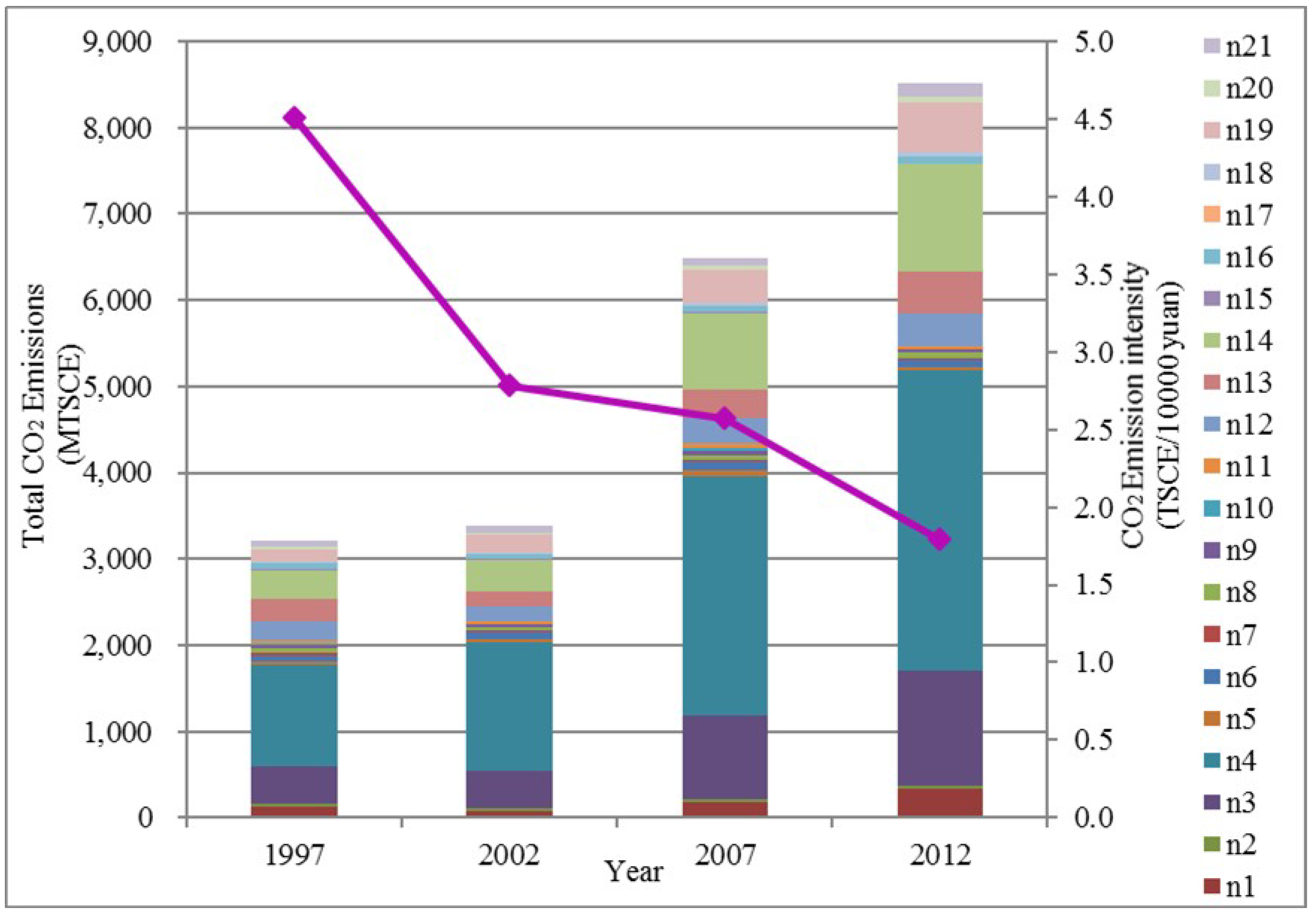
Based on the compiled IO tables, the trajectory of China’s production-based emissions (i.e., the TE in Equation (8)) and total emission intensity (i.e., the CEI in Equation (10)) for 1997–2012 can be obtained, as illustrated in Figure 2. Generally, China’s total emissions showed a consistent upward trend, from approximately 3206.23 million tons of standard coal equivalent (TSCE) in 1997 to 8506.85 million TSCE in 2012 at a growth rate above 165%. In contrast, China’s total emission intensity otherwise declined by approximately 60.1% from 4.50 to 1.79 TSCE/10,000 yuan for 1997–2012.

During different periods, the extents to which China’s CO₂ emissions (or total emission intensity) increased (declined) are at different levels. On the one hand, during the period 2002–2007, China’s total emissions climbed the most dramatically, whereas the emission intensity declined the slightest. The possible reason might lie in the large expansion of emission-intensity products (mainly corresponding to technology coefficient (B)), such as the products of processing of petroleum, coking, and nuclear fuel (n3) (with an 83.46% growth in output for 2002–2007), production and supply of electric power and heat (n4) (251.84%), non-metallic mineral products (n13) (269.16%), etc., which largely stimulated China’s emissions thereby suppressing the reduction of total emission intensity. On the other hand, during 1997–2002 and 2007–2012, China’s total emission intensity dropped quickly, and the emissions climbed moderately relative to 2002–2007. The latent factors might refer to various technological effects (particularly corresponding to energy technology) and structural effects (mainly regarding industrial structure and energy structure), and the top leading drivers will be explored by the proposed method later.

From the sectoral perspective, the estimated sectoral emissions are reported in Table S1 of the Supplementary data. According to the results, the top major emitters for 1997–2012 were consistently the sectors of processing of petroleum, coking, and nuclear fuel (n3), production and supply of electric power and heat (n4), chemical (n12), non-metallic mineral products (n13), smelting and pressing of metals (n14), and transport, storage, and post (n19). It is worth noticing that these six sectors made up the majority of China’s total CO₂ emissions. For example, the total emissions of the six sectors accounted for approximately 88.10% of China’s total emissions in 2012, and the largest emitter, i.e., production and supply of electric power and heat (n4), contributed approximately 40.92%. Interestingly, these six sectors are all emission-intensive sectors in terms of high direct-emission coefficients, respectively approximately 9.48, 9.07, 0.40, 1.27, 1.96, and 0.61 TSCE/10⁴ yuan in 2012. This implies that the direct-emission coefficient (C) might be a leading driver of China’s CO₂ emissions.

3.3. Top Overall Drivers of Emission Intensity Change

According to the proposed hybrid method (see Figure 1), the first step is to use SDA, an overall and ex-post analysis, for identifying the major overall drivers that “have” made the largest contribution to China’s total emission intensity change, as the analytic targets in the second step of sensitivity analysis. In comparison, the existing sensitivity analyses otherwise pre-determined target coefficients without a systematical quantitative analysis.

According to Equations (15)–(18), CEI can be decomposed into the changes of (1) direct-emission coefficient (C), (2) technology coefficient (B), (3) final demands structure by product (D), and (4) final demands by category (F). The detailed parameters are as shown in Equations (3)–(7) and (10)–(18).

Table 4. Contributions of different factors to China’s total emission intensity.

Factors (Equation)	Mark	1997–2002		2002–2007		2007–2012
		Change	C-ratio	Change	C-ratio	Change	C-ratio
Direct-emission coefficient (Equation (15))	C	0.6130	102%	0.7398	2711%	0.8655	40%
Technology coefficient (Equation (16))	B	0.9777	6%	1.2541	−2647%	0.8185	55%
Final demands structure by product (Equation (17))	D	1.0363	−10%	0.9953	49%	0.9497	15%
Final demands by category (Equation (18))	F	0.9931	2%	1.0012	−13%	1.0335	−10%
Total changes (Equation (14))	CEI	0.6168	100%	0.9245	100%	0.6953	100%

Notes: The product of the four factor-attributable changes are equal to the total changes. For example, the total change in emission intensity CEI in the period 1997–2002 is 0.6168 = 0.6130 × 0.9777 × 1.0363 × 0.9931. A change of coefficient above 1 indicates a negative effect on the reduction in total emission intensity, and a value below 1 corresponds to a positive effect. The contribution ratio (C-ratio) is calculated by dividing 1 minus the corresponding change value by the summation of 1 minus every change value [59]. For instance, the C-ratio of factor C in the period 1997–2002 is 102% = (1 − 0.6130) / [(1−0.6130) + (1−0.9777) + (1 − 1.0363) + (1 − 0.9931)]. A positive C-ratio indicates a positive effect on the reduction in total emission intensity, and a negative value implies a negative effect.

presents the decomposition results, in terms of the changes in coefficients and the corresponding contribution ratios (C-ratio) to the change of China’s total emission intensity. The detailed calculation process of the SDA results, together with illustrating examples, are provided in the notes of Table 4. From the results, one important conclusion can be deduced that the factors C and B, in terms of high absolute C-ratios, were two leading drivers of China’s total emission intensity.

During different periods, the leading drivers of China’s total emission intensity change were different. For the period 1997–2002, the decline of China’s total emission intensity was mainly caused by the factor C with the C-ratio of approximately 102%, while the absolute C-ratios of other factors were all below 10%. For the period of 2002–2007, the coefficients C and B, respectively with the C-ratios of approximately 2711% and −2647%, became the major factors largely impacting China’s total emission intensity. Notably, the absolute C-ratios for coefficients C and B in the period 2002–2007 were extraordinarily large, and the direct reason is that the associated factor-attributable changes in total emission intensity (i.e., 26.02% and 25.41%, respectively) were disproportionally larger than the overall change in total emission intensity (i.e., 7.55%). The great contribution of direct-emission coefficient C to the emission intensity decrease for 2002–2007 could be attributable to the considerable effort made by China to reduce total emission intensity, particularly in terms of promoting the use of renewable energy (e.g., biogas, geothermal energy, and tidal energy), upgrading coal-fired industrial boilers, and developing coal direct liquefaction technology [67]. In comparison, the large negative effect of technology coefficient B implies a deteriorating production structure during 2002–2007, mainly due to a large expansion of emission-intensive products [60]. For example, the production of steel was about 182.4 million tons in 2002; however, it jumped to 489.3 million tons in 2007. Similarly, the output of iron and cement increased by about 178.9% and 87.7%, respectively, during 2002–2007 [68]. For 2007–2012, the two factors B and C stood out again, explaining approximately 55% and 40% of the reduction in China’s total emission intensity, respectively, whereas the figures for other factors were in the range of [−10%, 15%].

The roles of different factors in China’s total emission intensity change can be then identified, and the two factors C and B are observed much more influential. First, the factor C is consistently tested to be a key driver of China’s total emission intensity change for all the sampling periods, with the C-ratios all above 40%. This result implies that the emission-intensive sectors, in terms of high sectoral direct-emission coefficients (c_i), should be especially targeted in mitigation policies. Second, the factor B played an extremely prominent role in China’s total emission intensity change, particularly for the periods after 2002 (with C-ratios all above 55%). Specifically, without carefully addressing the factor B (in terms of the expansion of emission-intensity products), although the factor C made a great effort to reduce China’s total emission intensity for 2002–2007, such a positive effect (in terms of a C-ratio of 2711%) was almost offset by the negative effect of the factor B (−2647%). In contrast, a large improvement in B (in terms of the highest C-ratio) for 2007–2012 effectively promoted China’s emissions mitigation, even with the relatively weak effects of other factors. Third, as for the other two factors, D and F, the effects on China’s total emission intensity change were relatively week, and their joint C-ratios were approximately 8%, 36%, and 5% for the periods of 1997–2002, 2002–2007, and 2007–2012, respectively.

Generally speaking, the SDA results indicate that the factors C and B were the top two leading overall drivers, which have contributed to 40% and 55%, respectively, of the changes in China’s total emission intensity during the whole sampling period 1997–2012. Such a contribution was substantially outstanding for the period 2002–2007, with absolute C-ratios even above 2000%. Interestingly, our finding is generally in line with prior studies [18,24,38], i.e., that the technology (B) and emission factors (C) were the top two leading drivers for changing China’s total emission intensity. Accordingly, an interesting question arises regarding how and to what extent these two determining factors will influence China’s total emission intensity, and the answer can provide helpful insights into designing specific, targeted mitigation policies for China. However, previous SDA-based studies have not addressed such an interesting question. Therefore, this hybrid method further introduces sensitivity analysis as a perfect complement to SDA, for further revealing how these two top drivers (identified by SDA) will impact future emission intensity from an ex-ante and sectoral perspective.

3.4. Key Sectoral Factors of Direct-Emission Coefficient

In the second step of the proposed approach, leading overall drivers of China’s total emission intensity change are investigated via an emerging ex-ante analysis—sensitivity analysis—to further capture their essential specific elements at sectoral levels. In contrast to the existing sensitivity analyses pre-determining the target coefficients without a systematical quantitative analysis, this study especially employs SDA to determine them as those “having” made the largest contribution to China’s total emission intensity change in the past.

In this section, the direct-emission coefficient (C) is explored for its sensitive sectoral elements—the key sectors which will exert significant influences on the factor C and hence China’s total emission intensity. Table S2 of Supplementary data lists the results of sectoral direct-emission coefficients c_i calculated based on the latest data (i.e., the IO table for 2012), and Figure 3 presents their corresponding elasticity values—${\epsilon }_{CEI,c_i}$, the extent to which a 1% change in c_i (the specific element of factor C in sector i) influences the total emission intensity. From the results, an interesting finding can be obtained that the key sectors for the factor C (in terms of large elasticities) are all emission-intensive sectors (in terms of high sectoral direct-emission coefficients). The parameter c_i is calculated by Equation (7), and its elasticity value can be obtained by Equation (23).

From Figure 3, it can be obviously seen that China’s total emission intensity is the most sensitive to the changes in the direct-emission coefficients of processing of petroleum, coking, and nuclear fuel (n3), production and supply of electric power and heat (n4), chemical (n12), non-metallic mineral products (n13), smelting and pressing of metals (n14), and transport, storage, and post (n19). Specifically, their elasticities ${\epsilon }_{CEI,c_i}$ all surpass 0.045%, while the figures for other sectors are below 0.020% except for coal mining and dressing (n1) (approximately 0.039%). The results indicate that a 1% improvement of the direct-emission coefficient in any one of the six sectors will reduce at least 0.045% of China’s total emission intensity. Interestingly, the direct-emission coefficients of the six sectors are all at high levels, respectively approximately 9.48, 9.07, 0.40, 1.27, 1.96, and 0.61 TSCE/10⁴ yuan in 2012. The hidden reason is easy to understand: according to Equation (23), the elasticity ${\epsilon }_{CEI,c_i}$ for the factor C is closely related to its sectoral elements, i.e., sectoral direct-emission coefficient (c_i). Furthermore, these six sectors are also the largest emitters of China’s emissions for 1997–2012 (see Figure 2). Therefore, the processing of petroleum, coking, and nuclear fuel (n3), production and supply of electric power and heat (n4), chemical (n12), non-metallic mineral products (n13), smelting and pressing of metals (n14), and transport, storage, and post (n19) can be identified as the key sectors that might lead to the highest growth in China’s emissions.

Such an insightful result at the sectoral level implies that China’s total emission intensity is the most sensitive to the changes in direct-emission coefficients of the six sectors, i.e., processing of petroleum, coking, and nuclear fuel (n3), production and supply of electric power and heat (n4), chemical (n12), non-metallic mineral products (n13), smelting and pressing of metals (n14), and transport, storage, and post (n19), which should be especially targeted when controlling the major driver C. Accordingly, a series of related measures are recommended to be carried out for reducing their sectoral direct-emission coefficients (c_i), which will effectively improve the direct-emission coefficient (C) thereby reducing China’s total emission intensity. Promising measures are extensive application of energy-efficient machinery and equipment in the emission-intensive industries [33], enhancing the share of cleaner fossil fuels such as natural gas and promoting renewable energy in energy input [60], encouraging cleaner technology innovation and adopting economic instruments such as taxes or subsidies [28].

3.5. Key Sectoral Factors of Technology Coefficient

The technology coefficient B is the Leontief inverse matrix, with elements b_i,k (or a_i,k) representing the direct or indirect demand for the goods and services produced domestically by sector i made by sector k [32]. For a target sector m, the associated elasticities, ${\epsilon }_{CE{I}_m,a_{i,k}}$ and ${\epsilon }_{CE{I}_m{}_{,}{a}_{i,k}}^{*}$, measure the extent to which the change in sectoral technology coefficient a_i,k influences the sectoral emission intensity $CE{I}_m$. Here, the six top emission-intensive sectors, whose sectoral emission intensities are the most significantly influential in terms of the total emission intensity (as identified in Section 3.4), are especially focused on as the target sectors. Two types of elasticities are considered—${\epsilon }_{CE{I}_m{}_{,}{a}_{i,k}}^{*}$ focusing on technological changes (see Equation (29)), and ${\epsilon }_{CE{I}_m,a_{i,k}}$ incorporating structural changes (see Equation (28))—which allow discussion of the technology coefficient B from the two perspectives of technological change and structural change, respectively. Accordingly, the “structure-relevant” technical coefficient elasticity (TCE) for factor B (technology coefficient), i.e., ${\epsilon }_{CE{I}_m,a_{i,k}}$ can be obtained by Equation (28). The “technology-relevant” TCE for factor B (technology coefficient), i.e., ${\epsilon }_{CE{I}_m{}_{,}{a}_{i,k}}^{*}$, can be obtained by Equation (29).

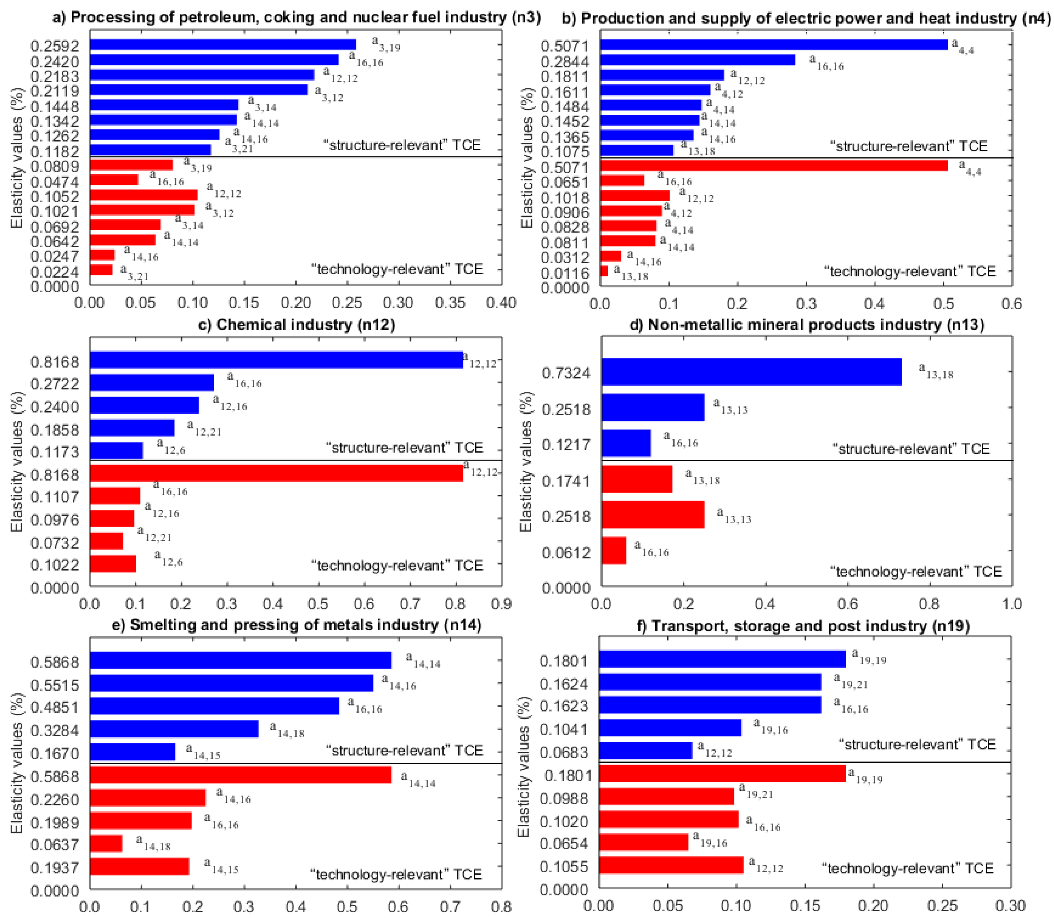
Figure 4 only shows the elasticity values ${\epsilon }_{CE{I}_m,a_{i,k}}$ of the essential technology coefficients with the threshold of 0.1 (i.e., ${\epsilon }_{CE{I}_m,a_{i,k}}>0.1$) [33], together with the corresponding “technology-relevant” TCE ${\epsilon }_{CE{I}_m{}_{,}{a}_{i,k}}^{*}$. For example, the result ${\epsilon }_{CE{I}_3,a_{3,19}}=0.2592$ means that a 1% improvement in the technology coefficient a_3,19 of the intermediate products provided by processing of petroleum, coking, and nuclear fuel (n3) less consumed by transport, storage, and post (n19) during the production process will reduce the emission intensity of n3 by approximately 0.2592%.

From Figure 4, one important conclusion can be drawn, which is that the emission intensities of the six key sectors, i.e., processing of petroleum, coking, and nuclear fuel (n3), production and supply of electric power and heat (n4), chemical (n12), non-metallic mineral products (n13), smelting and pressing of metals (n14), and transport, storage, and post (n19), are all the most sensitive to changes in technology coefficients of their own industries, in terms of the highest elasticity values (higher than 0.1%), i.e., the technology coefficients of the key six sectors with direct transaction relations have greater influences on the emission intensity than those with indirect transaction relations. In particular, the emission intensities of production and supply of electric power and heat (n4), chemical (n12), smelting and pressing of metals (n14) and transport, storage, and post (n19) are all the most sensitive to the technology changes of the intermediate products both produced and consumed by themselves; and those of processing of petroleum, coking, and nuclear fuel (n3) and non-metallic mineral products (n13) are the most significantly influenced by the technology changes of the self-supplied intermediate products but consumed by transport, storage, and post (n19) and construction (n18), respectively. These results repeatedly support the extremely crucial roles of the six key sectors in China’s emission intensity, which should also be targeted in particular when controlling the major driver B. Effective measures are suggested to reduce the activity levels and avoid surplus productions in these emission-intensive industries, such as enhancing environmental taxes, developing new energy conservation technologies and phasing out outdated technologies to reduce the loss rate in energy processing and conversion [60].

Through indirect transaction relations, some other industries might also exert significant influences on the emission intensity. An outstanding one is the manufacture of general equipment (n16) whose changes in technology coefficient consuming self-supplied intermediate products, i.e., a_16,16, will significantly influence the emission intensity of all six key sectors, and those consuming the intermediate products produced by smelting and pressing of metals (n14), chemical (n12), and transport, storage, and post (n19) are also influential. For example, apart from the direction transaction relations with the key six sectors, the elasticity of technology coefficient a_16,16 ranks first for production and supply of electric power and heat (n4) and chemical (n12), and second for processing of petroleum, coking, and nuclear fuel (n3), non-metallic mineral products (n13), smelting and pressing of metals (n14) and transport, storage, and post (n19). Interestingly, these results are consistent with the existing literature [32,33], in which the important role of manufacture of general equipment (n16) in China’s emission intensity were similarly observed via the sensitivity analysis of the technology coefficient. The hidden reason might lie in the production structure of manufacture of general equipment (n16). In particular, the products consumed by n16 accounted for approximately 13.20%, 7.85%, 31.97%, and 12.36% of the total consumption produced by chemical (n12), non-metallic mineral products (n13), smelting and pressing of metals (n14), and transport, storage, and post (n19) in 2012, respectively. Moreover, construction (n18) and transport, storage, and post (n19) are also worth noticing, whose changes in technology coefficients remarkably impact the emission intensities of non-metallic mineral products (n13) and processing of petroleum, coking, and nuclear fuel (n3), respectively.

When comparing the elasticity and its “technology-relevant” TCE, two interesting findings can be observed. On the one hand, there is a relationship ${\epsilon }_{CE{I}_m{}_{,}{a}_{i,k}}\gg {\epsilon }_{CE{I}_m{}_{,}{a}_{i,k}}^{*}$ for most technology coefficients, such as a_3,19 for processing of petroleum, coking, and nuclear fuel (n3) (i.e., ${\epsilon }_{CE{I}_3,a_{3,19}}=0.2592\%\gg {\epsilon }_{CE{I}_3,a_{3,19}}^{*}=0.0809\%$) and a_13,18 for non-metallic mineral products (n13) (with 0.7324% $\gg$ 0.1741%). This implies the emission intensities for these sectors are significantly impacted by the final demand structure, i.e., the technology coefficients will impose a stronger influence on China’s total emission intensity when considering the effect of final demand structure. Accordingly, the adoption of effective measures to improve final demand structure is advised when addressing the technology coefficients, such as energy structure improvement by promoting the use of cleaner fossil fuels instead of coal in energy input for the non-metallic mineral sector (n13) [60]. On the other hand, there are also two exceptions, i.e., a_14,15 for smelting and pressing of metals (n14) (with 0.1670% $\ll$ 0.1937%) and a_12,12 for transport, storage, and post (n19) (with 0.0683% $\ll$ 0.1055%), where ${\epsilon }_{CE{I}_m{}_{,}{a}_{i,k}}\ll {\epsilon }_{CE{I}_m{}_{,}{a}_{i,k}}^{*}$, otherwise supporting the importance of technological improvements. In these two peculiar cases, technology coefficients will influence the emission intensities mainly via the technological effect rather than the structure effect, and efficient measures for technological improvement are more desirable, such as introducing energy-efficient equipment (e.g., energy-saving cooling equipment in the smelting and pressing of metals sector (n14) [69]).

3.6. Subsection Data Descriptions

Based on the proposed hybrid approach, a rich array of new and interesting findings, i.e., drivers leading to the largest emissions at both overall and sectoral levels and from both ex-post and ex-ante perspectives, are explored. These outstanding factors constitute a map of hotspots in China’s energy system as shown in Figure 5, which can provide helpful insights into specific, targeted mitigation policies. In particular, the top leading drivers (i.e., C in Equation (3) and B in Equation (7)) and high elasticity value for these factors (i.e., ${\epsilon }_{CEI,c_i}$ in Equation (23), ${\epsilon }_{CE{I}_m,a_{i,k}}$ in Equation (28) and ${\epsilon }_{CE{I}_m{}_{,}{a}_{i,k}}^{*}$ in Equation (29)) can be highlighted.

The proposed hybrid approach first employs SDA to identify the top overall drivers that have largely impacted China’s total emission intensity for 1997–2012—direct-emission coefficient (C) and technology coefficient (B). This finding provides helpful insights into the major directions of mitigation policies for China—the government could reduce China’s emission intensity, by curbing key sectoral elements of driver C (i.e., direct-emission coefficients c_i of sector i) and driver B (technology coefficients a_i,j of emission-intensive sectors). To accordingly design the specific, targeted policies, sensitivity analysis is especially conducted to respectively explore the sectoral key elements of the two determine drivers, which will lead to massive future emissions. The corresponding results, together with promising measures, are as follows.

For driver C, the sensitivity analysis reveals that the emission-intensive sectors with the high direct-emission coefficients are the key sectors (in terms of large elasticity ${\epsilon }_{CEI,c_i}$), which will cause the highest CO₂ emissions: processing of petroleum, coking, and nuclear fuel (n3), production and supply of electric power and heat (n4), chemical (n12), non-metallic mineral products (n13), smelting and pressing of metals (n14) and transport, storage, and post (n19). According to Equation (23), the elasticity ${\epsilon }_{CEI,c_i}$ for driver C is determined mainly by sectoral direct-emission coefficient (c_i). Thus, policy measures, e.g., energy technology update and energy structure improvement, are strongly recommended for reducing the key sectoral direct-emission coefficients c_i (i = 3, 4, 12, 13, 14, 19), and thereby China’s total emission intensity to a largely proportional extent (according to the large elasticity ${\epsilon }_{CEI,c_i}$). Promising sector-specific measures are as follows: (1) introducing recyclable fluidized bed combustion technology in the chemistry industry (n12) [70]; (2) employing compressed air energy storage technology in the production and supply of electric power industry (n4) [71]; (3) promoting the use of solar energy in the non-metallic mineral industry (n13) [72]; (4) using biodiesel in the transport sector (n19) [73].

Regarding driver B, its key sectoral elements—the essential sector linkages a_i,k, whose changes will severely impact China’s total emission intensity—are deeply explored. First, the sensitivity analysis reveals that the emission intensities of the key sectors are the most sensitive to the changes in the technology coefficients of their own industries, i.e., the direction relations of a_4,4, a_12,12, a_14,14, and a_19,19 (with the highest elasticity ${\epsilon }_{CE{I}_m,a_{i,k}}$). Second, in indirect relations with the six key sectors, outstanding hotspots are the manufacture of general equipment industry (n16) whose changes in technology coefficient consuming self-supplied intermediate products a_16,16 exert significant influences on the emission intensities of all the six key sectors, and the construction industry (n18) and transport, storage, and post (n19) whose changes of technology coefficients greatly impact the emission intensities of non-metallic mineral products (n13) and processing of petroleum, coking, and nuclear fuel (n3), respectively. According to the nature of elasticity ${\epsilon }_{CE{I}_m,a_{i,k}}$, a 1% improvement in the technology coefficient a_i,k (i.e., the intermediate products provided by Sector i less consumed by Sector k during the production process) will reduce the emission intensity of Sector m by approximately ${\epsilon }_{CE{I}_m,a_{i,k}}$, and thereby China’s total emission intensity. Accordingly, reducing the activity levels of these sector linkages is a simple but efficient way to cut down China’s emission intensity, via efficient economic measures (e.g., environmental taxes) for these sectors that highly rely on the self-suppled intermediate products [60].

Based on Equation (28), the elasticity ${\epsilon }_{CE{I}_m,a_{i,k}}$ for driver B is impacted largely by the sectoral input (x_j) in addition to the technology coefficient (a_i,j). Thus, saving inputs (particularly energy inputs) and introducing new technology in the related sectors becomes another efficient way to improve technology coefficient (B) and hence China’s emission intensity. Possible sector-specific measures for energy conversation include: (1) using evaporative condenser and oxygen-enriched technology in the smelting and pressing of metals industries (n14) [67,74]; (2) introducing the straw pyrolysis gas technology in processing of petroleum, coking, and nuclear fuel (n3) [75]; (3) promoting ground source heat pump in the construction industry (n18) [76].

4. Conclusions and Policy Implications

To systematically investigate the drivers of China’s CO₂ emission intensity change, this study might be the first attempt to couple SDA and sensitivity analysis to propose a hybrid approach. Generally, the major contributions of this work to the literature can be summarized in the following two ways. First, the hybrid approach not only explores the major drivers of China’s total emission intensity change at an overall level and from an ex-post perspective as did most previous studies for China, but also probes each top leading driver to identify its essential specific elements at a sectoral level and from an ex-ante perspective via the promising method of sensitivity analysis. Second, four hybrid physical-monetary energy IO tables in China for 1997, 2002, 2007, and 2012 are compiled, to not only capture the long-term trends for 1997–2012 in the ex-post analysis, but also conduct the ex-ante analysis based on the most updated data for 2012. In particular, the proposed method is implemented to explore the drivers of China’s CO₂ emission intensity change and provide a hotspot map of energy systems for specific, targeted mitigation policies. From the ex-post perspective, SDA is implemented to identify the top overall drivers that have largely affected total emission intensity, i.e., direct-emission coefficient (C) and technology coefficient (B). The results point out the major directions to control China’s emission intensity-curbing key sectoral direct-emission coefficients (regarding C) and technology coefficients (regarding B). From the ex-ante perspective, the hybrid method introduces sensitivity analysis to deeply investigate the two drivers at sectoral levels, revealing which essential sectoral factors will lead to massive future emissions. For the driver C, the sensitivity analysis reveals that the high emission-intensive sectors are the key sectors which will cause the highest emissions: processing of petroleum, coking, and nuclear fuel (n3), production and supply of electric power and heat (n4), chemical (n12), non-metallic mineral products (n13), smelting and pressing of metals (n14), and transport, storage, and post (n19). Regarding B, the emission intensities are the most sensitive to the changes of the technology coefficients in the direct relations with the six key sectors. Accordingly, China should make a great effort to control the emission intensities and the activity levels of the six key sectors, thereby significantly reducing the total emission intensity. The empirical study provides new valuable findings for designing and adjusting specific, targeted mitigation policies for China.

However, there are still many interesting works for the future research. First, the empirical study especially focuses on China, and the hybrid method could be applied to other regions, states, and cities in the world to verify its generalization and universality. Second, in SDA, some other important factors, such as population change and per-capita carbon emission, could also be considered. Third, the sensitivity analysis only investigates the top two leading drivers, and a comprehensive analysis for various factors is desirable. We will consider these interesting issues in the near future.