A 3D Numerical Study of Supersonic Steam Dumping Process of the Pressurizer Relief Tank

Abstract

Simulating the steam dumping process of a pressurized relief tank is a challenging engineering problem, due to the massive computing resource requirements and its complex physical models. This study gave a comprehensive 3D numerical study for the transient dumping process from the PRT (Pressurizer Relief Tank) to the room containing the tank. The physical model, geometry design and meshing strategy, along with the numerical techniques, have been described in detail. Through parallel simulations based on the open source CFD toolbox OpenFOAM, numerical results for the temperature, pressure, and the velocity distribution are presented. The results show that the maximum velocity throughout the whole domain is 967 m/s over Mach 2 and the maximum pressure on the roof of the room is 2.8 atm. It could provide the guidance information for the safety design of the reactor coolant system. Additionally, comparison cases between OpenFOAM and CFX are tested, and it turns out that OpenFOAM could produce comparable accuracy with commercial CFD software and scale to much more computing cores in parallel simulations.

1. Introduction

A PRT is a large tank containing water with a nitrogen atmosphere. As one of the important components in the reactor coolant system, the PRT along with the pressurizer plays a significant role in controlling the system pressure. The PRT has been in the area of industrial engineering for the quench spray system of nuclear reactors [1], reactor coolant system of PWR (Pressurized Water Reactor) [2] and hydrogen mitigation systems [3]. The PRT is connected with the pressurizer of a pressurized-water coolant system through safety valves [4]. When the pressure in the pressurizer continues to increase and exceeds the threshold, the relief valves will open and dump steam to the pressurizer relief tank. Typically, the steam could dump into a concrete room (interior space) through the vent outlet while the pressure exceeds the safety point [5].

Simulating the steam dumping process of the PRT faces many challenges. Firstly, the geometry of the simulation domain is complex. There are three components: a large cylinder, two semicircles on either side of the cylinder and two vents on the cylinder. The upper part of the PRT is an air chamber which is filled with steam. Simulating the fluid dynamics in such a complex geometry requires at least millions of mesh cells. Making an efficient and large-scale collaboration for real world complex CFD (Computational Fluid Dynamics) applications is still a problem as hard as any that computer science has faced [6]. Secondly, the multi-component gas in the tank and the supersonic outlet airflow bring difficulties to accurately model the complex flow phenomena. In the dumping process, the steam flows out from the PRT, spreads into the concrete room, whilst the steam will be accelerated to a supersonic speed. Thus, we cannot ignore the change in steam density [7]. Meanwhile, the thermal energy change is also an important factor affecting steam density and viscosity. The scholars used to consider the heat transfer process in different situations, like the analysis of the flow inside of the VMU(Video Management Unit) MkII which is an electronic box located in the International Space Station [8] and the analysis of thermal-hydraulic behaviour of the high performance light water reactor fuel assembly [9].

In practice, most of the numerical CFD study is based on the commercial software such as CFX. Nevertheless, due to the exorbitant price and the limitations on the parallel scale of the licenses, using a well-developed commercial software cannot meet all the requests of engineering design and testing. In addition, we also cannot integrate state-of-the-art models to accurately capture some fluid dynamic features in a complex geometry. Correspondingly, there is less limit for the parallel scale and the physical model extension with the open source software OpenFOAM.

Modern supercomputers are made up of millions of computing cores, and the mainstream CFD software cannot be executed on such a large scale hardware platform. To explore the potential parallel performance of the application and accurately capture more detailed fluid dynamics with finer mesh among larger domain, this study focuses on simulating the complex supersonic steam dumping process based on an open-source CFD software, OpenFOAM. Previous research showed the OpenFOAM could be used to solve engineering problems [10]. 3D numerical results will be presented in detail and the speedup will be analyzed on different parallel scales. Additionally, we compared the results between OpenFOAM and CFX.

The simulation is still based on single phase flow, so the details in steam–water behaviour is unclear. In practice, heat transfer on the wall of steam nozzles and chamber has an effect on steam flow, which is extremely complicated. Solving these problems is our future work and our present work is making the simulation of PRT achieved with OpenFOAM and CFX. The comparison of results is also discussed scientifically. Based on the simulation, the results and discussion can help provide reference data for the construction of PRT and make a contribution to the safe operation of nuclear reactors.

2. Numerical Method

2.1. Governing Equations

In a realistic system, the PRT is filled with multi-component steam. For simplicity, in our prototype simulation system, the fluid is described through the single phase compressible idea gas model for the reason that the velocity is detected over Mach 2. The flow simulation and heat transfer problem are described by the mass, momentum and energy equations. The mass equation is defined as the correlation between velocity and mass, which can also be called continuity equation and could be described as

$$\frac{\partial \rho }{\partial t}+\nabla ·\left(\rho \mathbf{U}\right)=0,$$

(1)

where $\rho$ is the mass of matter in each per unit volume and U represents the velocity. A differential to $\rho$ means how much mass of matter changed in the selected unit volume by time. The second term is the divergence of the product of fluid density and velocity.

The momentum balance equation can be written as

$$\frac{\partial \left(\rho \mathbf{U}\right)}{\partial t}+\nabla ·\left(\rho \mathbf{U}\mathbf{U}\right)=-\nabla p+\nabla ·\mathit{\tau },$$

(2)

where the first term is based on Newton’s Second Law. $\rho$U is explained as the reflection of velocity energy. The next term is Laplace transformation which means that the equation is in non-conservation form. $\mathit{\tau }$ is viscosity pressure tensor, and its unit is Pa. This equation shows the change of kinetic energy, where $\mathit{\tau }$ is given by

$$\mathit{\tau }=2\mu dev\left(\mathbf{D}\right),$$

(3)

$$\mathbf{D}=\frac{1}{2}[\nabla \mathbf{U}+{(\nabla \mathbf{U})}^T],$$

(4)

$$dev\left(\mathbf{D}\right)=\mathbf{D}-\frac{1}{3\mu }\nabla \mathbf{U},$$

(5)

where $\mu$ is kinetic viscosity, which reflects the internal friction force of material molecules. The dev(D) makes the gradient tensor of $\mu$.

The energy equation aims to solve the heat transfer problem. The thermal energy affects the state of steam, which is connected with the distribution of energy, density, enthalpy, and viscosity. The connection between enthalpy and pressure can be expressed by

$$e=h-p/\rho ={\int }_{T0}^T{c}_{v}dT-R_{u}T/W,$$

(6)

where h is the sum of thermal energy and pressure in unit mass. Sensible enthalpy depends on the temperature difference between the outside and inside of PRT. $c_v$ is specific heat capacity, and the next term is the energy of the gas at its current temperature. E is made up of thermal energy and kinetic energy using

$$E=H-p/\rho =e+1/2(\mathbf{U}·\mathbf{U}),$$

(7)

$$H=h+\frac{1}{2}\mathbf{U}·\mathbf{U},$$

(8)

$$\frac{\partial \rho e}{\partial t}+\nabla ·\left[\mathbf{U}\left(\rho e\right)\right]+\nabla ·q+(p-\mathit{\tau })\nabla ·\mathbf{U}=0,$$

(9)

$$q=-\lambda T,$$

(10)

where kinetic energy here is in unit mass and $\lambda$ is thermal conductivity. E is the sum of thermal energy and kinetic energy. e represents potential energy. H indicates total enthalpy change. h is sensible enthalpy change. Based on observations of both pressure p and temperature T, we assume the perfect gas fill PRT and interior space using

$$e=c_{v}T,$$

(11)

$$T=\frac{1}{c_v}[E-\frac{1}{2}\mathbf{U}·\mathbf{U}].$$

(12)

2.2. Turbulence Model

The compressible flow is simulated with the RANS (Reynolds Average Navier–Stokes) models and the RANS equations consist of the continuity and momentum equations. The turbulence model we choose is the $k-\omega$ Shear Stress Transport (SST) model which earns its fame by rallying the best of two families of turbulence models, the $k-ϵ$ and the $k-\omega$, and switches between the standard $k-ϵ$ model in the free-stream and the Wilcox’s $k-\omega$ model in the near-wall region which makes it valid all the way down to the wall [11]. There are two main reasons for choosing the SST model. First, the SST model is widely used in our previous research for studying the thermohydraulics phenomena in a nuclear reactor. The results showed that the accuracy and computational efficiency satisfied our requirements. Second, in a PRT simulation of the manuscript, we only focused on some statistical variable (such as the maximum/average pressure on the roof), and the internal details of the fluid flow are insignificant. Thus, using a classical two-equation SST model should be a good economic choice in this case.

The $k-\omega$ SST equations is a two-equation eddy-viscosity model described below:

kinematic eddy viscosity,

$${\nu }_t=\frac{a_{1}k}{max(a_1\omega ,S{F}_2)},$$

(13)

turbulence kinetic energy,

$$\frac{\partial k}{\partial t}+\frac{\partial \mathbf{U}k}{\partial x}-\frac{\partial \left[(\nu +{\sigma }_k{\nu }_t)\frac{\partial k}{\partial x}\right]}{\partial x}=P_k+{\beta }^{*}\omega k,$$

(14)

turbulent dissipation rate,

$$\frac{\partial \omega }{\partial t}+\frac{\partial \mathbf{U}\omega }{\partial x}-\frac{\partial \left[(\nu +{\sigma }_{\omega }{\nu }_t)\frac{\partial \omega }{\partial x}\right]}{\partial x}=\alpha S^2-\beta {\omega }^2+2(1-F_1)\frac{{\sigma }_{\omega 2}}{\omega }\frac{\partial k}{\partial x}\frac{\partial \omega }{\partial x},$$

(15)

with the coefficients ($F_2$, $P_k$, $F_1$, $C{D}_{k\omega }$) defined as follows:

$$P_k=min(\mathit{\tau }\frac{\partial \mathbf{U}}{\partial x},10{\beta }^{*}k\omega ),$$

(16)

$$F_1={\left\{min[max(\frac{\sqrt{k}}{{\beta }^{*}\omega y},\frac{500\nu }{y^2\omega }),\frac{4{\sigma }_{\omega 2}k}{C{D}_{k\omega }{y}^2}]\right\}}^4,$$

(17)

$$F_2=tanh\left({\left[max(\frac{2\sqrt{k}}{{\beta }^{*}\omega y},\frac{500\nu }{y^2\omega })\right]}^2\right),$$

(18)

$$C{D}_{k\omega }=max(2\rho {\sigma }_{\omega 2}\frac{1}{\omega }\frac{\partial k}{\partial x}\frac{\partial \omega }{\partial x},{10}^{-10}).$$

(19)

The parameters like $\alpha$, $\beta$, ${\sigma }_k$ and ${\sigma }_{\omega }$ are set from the Equation (20) by replacing $\varphi$ with the respective parameters [12]:

$$\varphi ={\varphi }_1{F}_1+{\varphi }_2(1-F_1).$$

(20)

Other parameters used above are selected as standard:

${\alpha }_1$ = 0.31, ${\alpha }_2$ = 0.44, ${\beta }_1$ = 0.075, ${\beta }_2$ = 0.0828, ${\beta }^{*}$ = 0.09, ${\sigma }_{k1}$ = 0.85, ${\sigma }_{k2}$ = 1, ${\sigma }_{\omega 1}$ = 0.5, ${\sigma }_{\omega 2}$ = 0.856.

3. Mesh Solution

3.1. Simulation Domain and Mesh

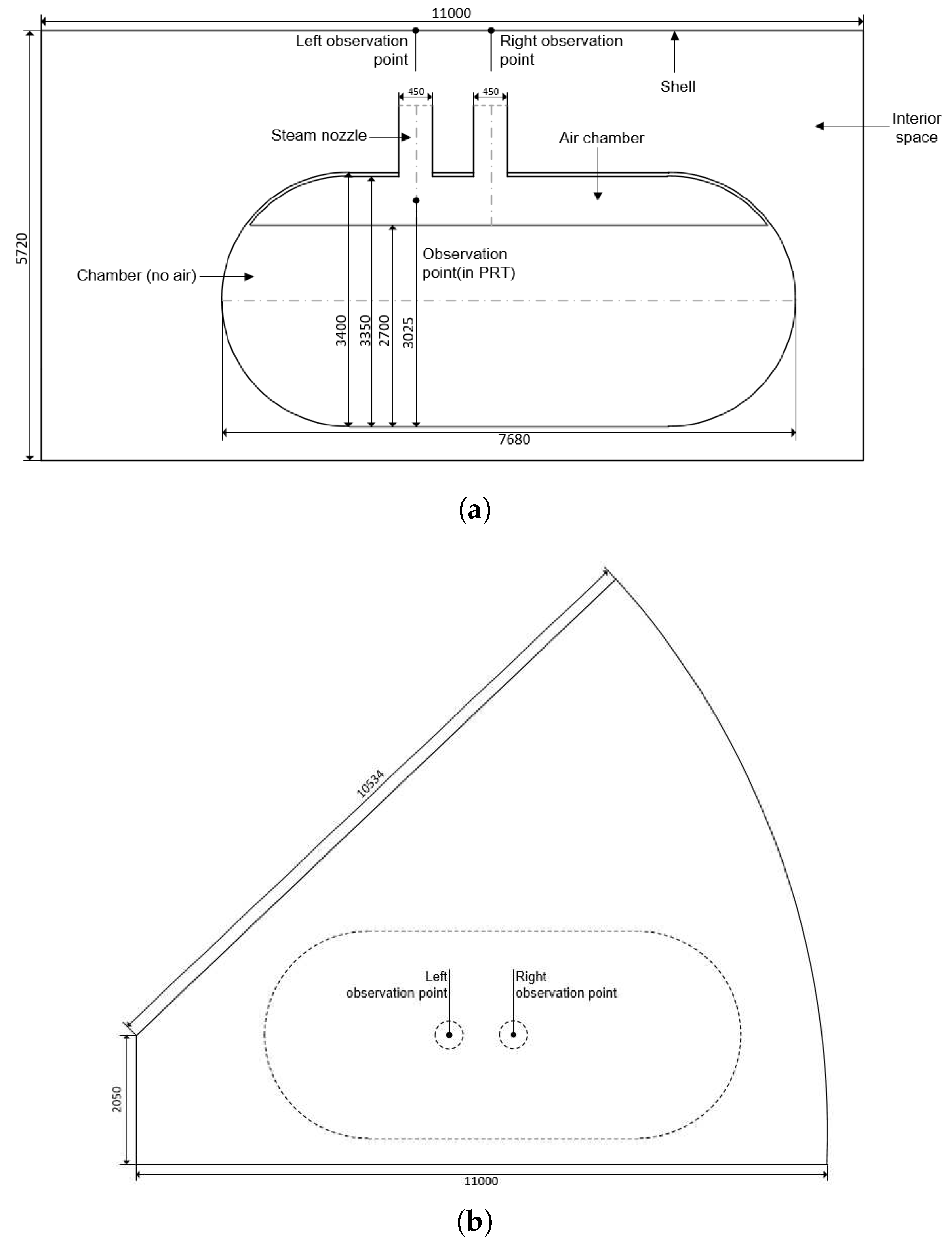
The numerical model of PRT and the shell is shown in Figure 1; in addition, all the parameters of geometric configuration and the locations of the observation points are marked. The parameters of geometric configuration are similar to real-world building and the PRT consists of three parts: steam nozzles, air chamber, and chamber (no air). The steam nozzles are the only channel connecting PRT and interior space.

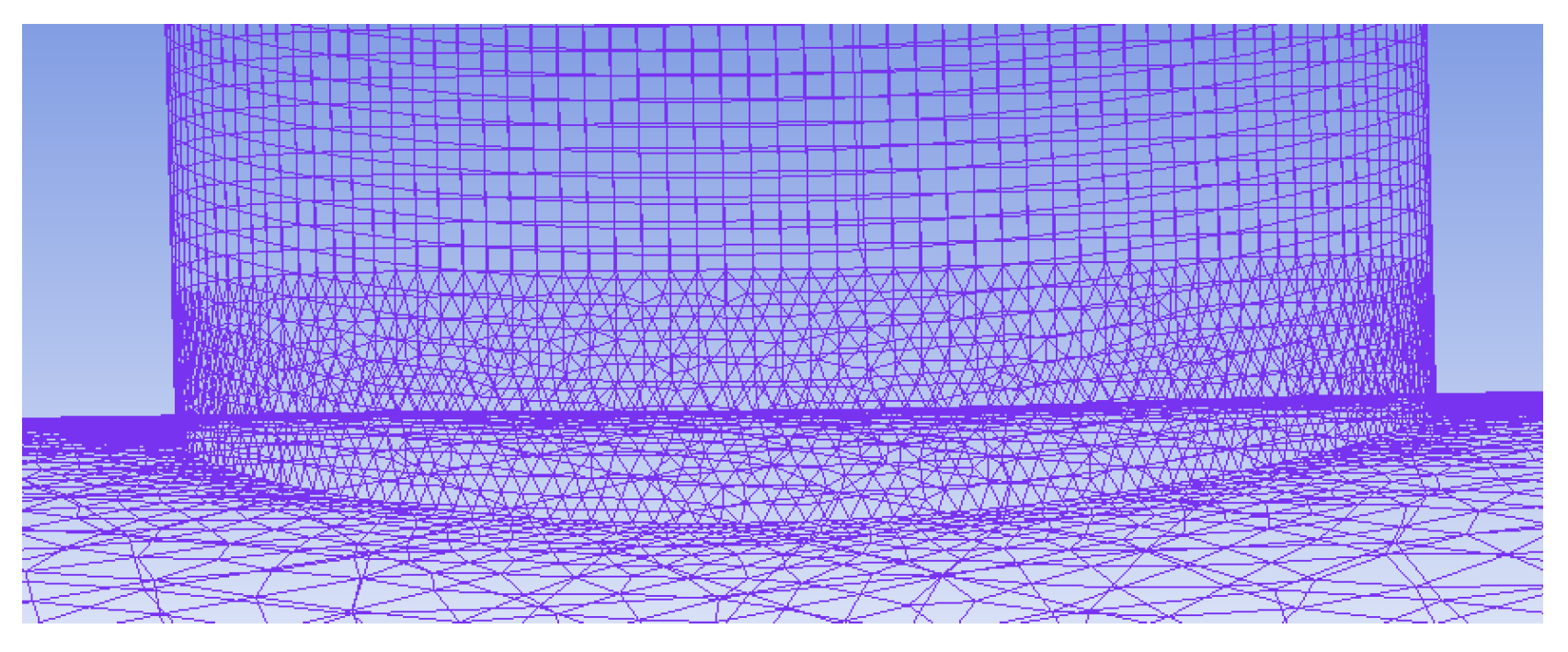
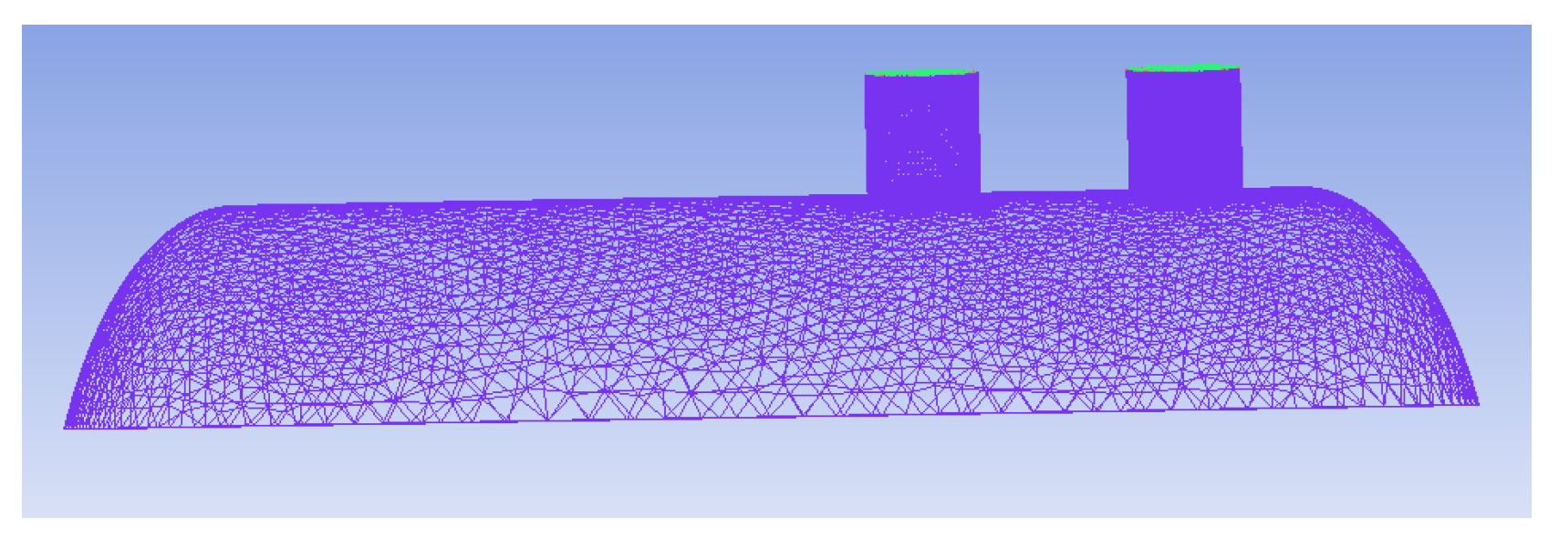
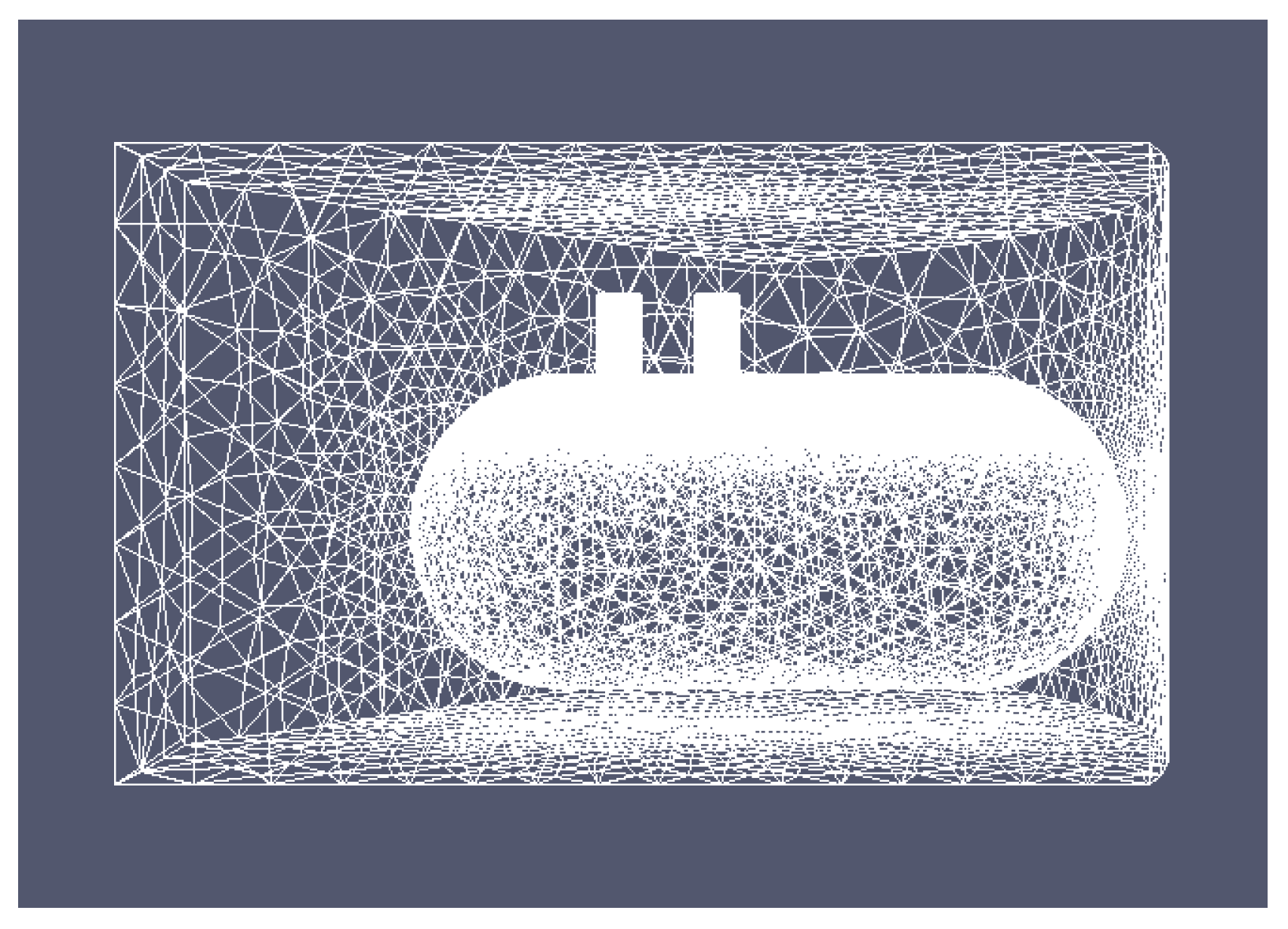
The quality and density of mesh are the vital factors of simulation accuracy and efficiency. Hybrid structured and unstructured mesh strategy are used in the meshing process. Meshes for the simulation domain are generated using ANSYS ICEM. For preserving y${}^{+}$ at the wall, we make special refinement and use unstructured grid to reduce the generating time cost at joints, as shown in Figure 2. The overall simulation mesh is shown in Figure 3, and the simulation mesh of air chamber is shown in Figure 4.

Normally, a special refinement should be made at the location where the steam flow has violent changes. Successive refinement due to curvature and proximity is the key to reasonably distributing nodes along curves so as to form well shaped elements [13]. The proximity and curvature refinement is made to solve the sector of the shell and the joints of cylinder and semicircle. The boundary layer is refined to five layers and the thickness growth rate of layer is set as 1.2. Another location we make refinement to is the joint of cylinder and vent, which is shown in Figure 2. Actually, in this location, we use unstructured topology to accelerate the solving speed.

3.2. Mesh Independency Check

The mesh independency check is made by the temperature of the observation point in PRT under three different mesh numbers of 1062520, 3804587, and 5216999. The comparison is shown in Figure 5. The similar profiles of the temperature can be predicted and the middle number of cells is chosen for calculation correctness and appropriate time step.

3.3. Numerical Algorithm and Scheme

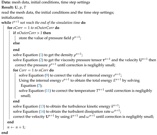
The solvers in OpenFOAM have both pre- and post-processing, and it provides a variety of finite volume solvers for structured grid and unstructured gird [14]. In order to design the solver and implement the compressible Navier–Stokes (N–S) equations, we select the PIMPLE algorithm to be implement in OpenFOAM, which is shown in Algorithm 1.

The sign of termination is the runTime to reach the endTime. Actually, there are two cycles and we input the values to nOuterCorr and nCorr. nOuterCorr is the number of pressure correction and nCorr is the number of piso algorithm solution, which is the implementation of the solution principles. Every time step, the solver will run this process.

Normally, the solution strategy is four steps, solving the velocity equation to get the velocity predicted value, using the value to correct the pressure, solving the energy conservation equation to correct the temperature, and then using pressure to correct the velocity. This strategy is used for compressible flow, incompressible flow, heat transfer and so on. The implementation is different depending on the specific object scheme.

Algorithm 1: The iterative algorithm to solve the compressible idea gas fluid model for simulating the steam dumping process.

Density is dynamically changed so we set the thermal setting to calculate density per unit time. The parameters of steam shown in

Table 1. The steam in high speed has different characters to gas at room temperature like low density and high specific heat.

Parameter	molWeight (kg/mol)	Cp (kJ) ${}^1$	Hf ${}^2$	As ${}^3$	Ts (K) ${}^4$
Value	18.02	3011	0	1 × 10${}^{-5}$	273

${}^1$ Cp = Specific Heat Capacity; ${}^2$ Hf = Enthalpy Change; ${}^3$ As = Sutherland Coefficient; ${}^4$ Ts = Reference Temperature.

are consistent with real situation.

The thermal model will help us to get the information of steam by those dynamic parameters. In the OpenFOAM file system, fvSchemes is the target file that contains the discretization schemes shown in

Table 2. fvSchemes setting will affect calculation accuracy and computational stability.

Parameter	Value
ddtSchemes	backward
gradSchemes	Gauss linear
divSchemes	Gauss linearUpwind Gauss linear (almost all)
laplacianSchemes	Gauss linear corrected
interpolationSchemes	linear
snGradSchemes	corrected
wallDist	meshWave

.

The file named fvSolution records the solver’s parameter. In addition to selecting the right solution, discrete formats have close correlation. The file content is in

Table 3. fvSolution contains a series of sub-dictionaries to afford the necessary info for the solvers’ running.

Domain	Solver	Preconditioner	Tolerance	RelTol
rho($\rho$)${}^{\mathbf{1}}$	diagonal	non	non	non
P${}^{\mathbf{2}}$	PBiCG	DILU	1 × 10${}^{-8}$	0
U${}^{\mathbf{3}}$	smoothSolver	symGaussSeidel	1 × 10${}^{-8}$	0
e${}^{\mathbf{4}}$	smoothSolver	symGaussSeidel	1 × 10${}^{-8}$	0
k${}^{\mathbf{5}}$	smoothSolver	symGaussSeidel	1 × 10${}^{-8}$	0
omega${}^{\mathbf{6}}$	smoothSolver	symGaussSeidel	1 × 10${}^{-8}$	0

${}^1$$\rho$ = Density; ${}^2$ P = Pressure; ${}^3$ U = Velocity; ${}^4$ e = Kinetic Energy; ${}^5$ k = Turbulent Energy; ${}^6$ omega = Attenuation Coefficient.

.

There is no limiting conditions for density, so we choose diagonal as it is the most simple solver. Usually, time derivative and Laplace item will use the symmetric matrix to solve, but, if the convection item exists, we have to use an asymmetric matrix. Thus, PBiCG is selected for calculating pressure. Relative tolerance should be zero as tolerance is the only standard to check whether the result is accurate. For tolerance, we set the value to 1 × 10${}^{-8}$ because usually 1 × 10${}^{-4}$ is enough for normal conditions, but this may be unsteady, which is why we should set a smaller value.

Delta time is also a difficult problem we should think about. Normally, this parameter needs to follow the CFL condition (the CFL condition: the CFL condition is named after Courant, Friedrichs, and Lewy, which is that a numerical method can be convergent only if its numerical domain of dependence contains the true domain of dependence of the PDE(Partial differential equation), at least in the limit as dt and dx go to zero.) [15]. The automatic adjustment in OpenFOAM can also help us to confirm and approach the most appropriate value of the DeltaT. As the result, we choose 5 × 10${}^{-7}$ s as the value of DeltaT. The file named controlDict records the content of running settings in

Table 4. fvSolution contains a series of sub-dictionaries to afford the necessary info for the solvers’ running.

StartTime	EndTime(s)	DeltaT(s) ${}^1$	WriteControl ${}^2$	WriteInterval ${}^3$
0	0.02	5 × 10${}^{-7}$	runTime	2 × 10${}^{-4}$

${}^1$ DeltaT = time step of the simulation; ${}^2$ WriteControl = controls the timing of write output to file; ${}^3$ WriteInterval = Scalar used in conjunction with Writecontrol.

.

In order to make the comparison representative, the simulation in CFX is of vital significance and the similar settings and parameters are expected to reduce systematic error. As the speed is predicted to reach supersonic, the first-order upwind advection scheme is chosen for the discretization of conservation equations. The material properties including equation of state, specific heat capacity, and transport properties can be considered as a real gas model with high velocity and high temperature, which are listed in

Table 5. Thermodynamic Properties in ANSYS-CFX material properties.

Options	Equation of State		Specific Heat Capacity		Transport Properities
	Option	Molar Mass	Value	Type	Option	Ref.TEMP
Value	Ideal Gas	18.02	3011	Constant Pressure	Sutherlands Formula	25

.

The fluid models is related to heat transfer settings and turbulence model, and the details are in

Table 6. Options in ANSYS-CFX fluid properties.

Options	Heat Transfer	Turbulence
	Option	Option	Wall Function
Value	Total Energy	Shear Stress Transport	Automatic

.

4. Results and Discussion

4.1. 3D Transient Simulation Results Based on OpenFOAM

The computation is running on a cluster consisting of more than 400 computing nodes, and the specification of a computing node is listed in

Table 7. Specifications of a computing node in the HPC (High Performance Computing) cluster.

Number of Processors	Specification of Each Processor	Cpu MHz	Cache Size (KB)
12	Intel(R) Xeon(R) CPU E5-2620 v2	2099.781	15,360

and the operating system used is the Red Hat Enterprise Linux Server release 6.5 (Santiago).

The steam in PRT and in interior space have different initial states shown in

Table 8. The initial state of the steam.

Location	Pressure (atm)	Temperature (${}^{\circ }$C)
In the PRT${}^{\mathbf{1}}$	16	200
In interior space	1	25

${}^1$ the PRT = the pressurizer relief tank.

. The setting is familiar to the real situation and we have already described the thermal parameters for calculating fluid density and fluid viscosity(nu).

The transient simulation results of the steam dumping process from the PRT into the shell room are presented here. As shown in Figure 6, the air jet is rapidly accelerated as driving by the pressure and temperature between the domain areas. To visually describe the whole process of steam dumping, Figure 6 shows the velocity snapshots from the simulation time $t=0.002$ s to $t=0.018$ s. The pressure difference is up to 16 atm which makes the high pressure steam gains a supersonic speed while it is dumped into the room. An area where the steam gains the maximum velocity continues to expand until the steam reaches the top of shell and diffuses along the top.

The whole dumping process could be divided into four primary stages from the observed numerical data. Figure 7, Figure 8, Figure 9 and Figure 10 represent a typical snapshot of the physical fields for these stages, respectively.

Figure 7 shows the steam beginning to spray out from the vents. At the first stage, the steam sprays out and rapidly exceeds the speed of sound to 821 m/s. We can see that the steam at the edges of the vents has maximum velocity. More details are direction of the steam flow and speed distribution. The steam near the pipe wall has not been greatly affected, while the steam from the PRT pushes the steam above the vents spread to the surroundings. In vents, the pressure is 4.0 atm and the velocity at the centre of vents is 600 m/s. At this time, steam in other space in the interior space has not been affected. The pressure and temperature distribution have a significant gradual process. In particular, pressure distribution is not monotonous and a low pressure zone appears in the middle of the steam flow. At the same time, the pressure on the top of the shell continues to rise.

Figure 8 shows the steam flow reaching the top of the shell. When the time goes to 0.004 s, the flow has been accelerated and the pressure to the roof reached the first peak, which is over 2.5 atm. The pressure inside the vent continues to decrease due to the steam spraying out. The low pressure zone in the middle of the flow corresponds to a high speed area.

In addition, the temperature is the same distribution that the temperature near the top is up to 122 ${}^{\circ }$C and still a low temperature field exists. It is absolutely possible as steam in this area gets the fastest speed to move away so that it is hard to gather steam and keep the constant temperature. At this time, we can notice that the steam flows out from the left vent gives higher pressure on the top since the shape of the shell and its location in the PRT. The areas directly above the vents on the top receive different pressure; the left is equal to 2.58 atm and the right is equal to 2.50 atm. The maximum speed of flow this time is 896 m/s and the location is rightly at the low temperature field.

Figure 9 shows that steam flow at this time is very representative as the steam spreads significantly around the top. The pressure at two key points is equal to 2.84 atm and 2.82 atm. In addition, we care about the velocity of steam in vents and the maximum value; in the centre of the vents, the speed is 510 m/s while the maximum is 895 m/s. This is a sign that the steam flow is spreading out on the top when the pressure on the top comes to the second peak.

Figure 10 is the last period which shows a typical state after 0.0052 s during the flow spread on the top. We can observe that the two key points we monitor float around 2.7 atm. The velocity at the center of vents is 650 m/s while the maximum is 967 m/s. We can notice that the pressure and temperature correspond, which conforms to physical laws. In PRT, the temperature drops to 162 ${}^{\circ }$C and there is an area on the top where the steam flow accumulates heat energy around 140${}^{\circ }$ at the location between two observation points. In addition, this period still has some fluctuations like at 0.072 s the pressure reduce to 2.32 atm, while, at 0.014 s, it is back to 2.8 atm again. The reason could be due to the formation of constant temperature zone on the top.

To sum up, the force on the roof is gradually increasing as the steam dumping progresses, and the pressure inside of the tank has dropped apparently as the pressurized steam flowing out into the interior space. The complete detailed 3D numerical results could be obtained from the simulations based on the OpenFOAM.

4.2. A Comparison between OpenFOAM and CFX

The pressure on the top of the shell is very representative and meaningful data. The two observation points are in circles each with an area of 1 m${}^2$ on the top right above two centres of vents. Because of the shape of the shell, the pressure on the left point is a little bit larger than the right one, while the trend is consistent. The results still have many differences which may be due to the differences of the basic solving mechanisms and the turbulence parameters, although the similar schemes are chosen in OpenFOAM and CFX. In OpenFOAM, we need to set a fixed value for the turbulence parameters as the initial setting, which will be dynamically solved in CFX.

Figure 11 shows the pressure–time curve of the right observation point. The process can be divided into four periods just as we described in the previous chapter. Here, we focus on the differences between two results on OpenFOAM and CFX. We can see CFX is smaller than OpenFOAM most of time. In addition, the fluctuation of CFX is more volatile than OpenFOAM. Especially between 0.008 s and 0.016 s, we can see that the OpenFOAM is smoother and has a peak at 0.016 s. Instead, CFX has no obvious peak and the floating range is smaller. After 0.013 s, OpenFOAM continues to grow and gradually becomes stable, while the CFX grows after 0.016 s. Overall, OpenFOAM and CFX have the same trend basically, but CFX seems much more sensitive.

Figure 12 shows the process of the temperature change in the PRT. With Figure 12, we can notice that the pressure of the roof circle rises quickly when the temperature in the PRT drops fast. At the beginning of the process, the steam in the vents is exhausted so the temperature in the PRT has no change. Because of the high pressure in the PRT, the steam in the PRT is vented rapidly after the steam in the vents has been exhausted. The change of temperature becomes relatively stable as the steam flow hits the roof and gets resistance. The spread of steam in interior space makes the temperature in the PRT drop continually. The prediction of CFX drops faster than the prediction of OpenFOAM, while the prediction of OpenFOAM is relatively stable. The reason for these performances may be the differences in discrete solutions, and it is not completely clear now.

For these differences, the reasons we consider are listed below: first, OpenFOAM is based on a conventional Finite Volume Method (FVM) while CFX is developed on an element based FVM (ebFVM). The approaches to the discretization of Navier–Stokes equations directly affect the computational performance. OpenFOAM achieves the spatial discretization by using FVM on block structured meshes with Gaussian integration and linear interpolation, but CFX employs an element based Finite Volume approach to discretize in space and the high resolution scheme is chosen for the stabilization of the convective term. This makes a difference in numerical calculations [16]. Second, the solving algorithm is different. OpenFOAM used the iterative algorithms (such as PISO, SIMPLE) to solve governing equations and the CFX implemented a full-coupled solver which solves the equations as a single system which eliminated the iteration process and improved the convergence speed. This may cause some differences in accuracy of solutions.

Overall, the simulation results showed a consistent trend with the CFX tests. Through the comparison, it could be concluded that the numerical solver based on OpenFOAM produces comparable accuracy with commercial CFD software for the PRT simulations.

4.3. Parallel Performance Tests Based on OpenFOAM

Powerful parallel expansion capability is a prime advantage compared to CFX, thus we test the case on a parallel computer and analyse the performance and scalability. Using one computing node (12 processors) to run the OpenFOAM solver, the execution time would be around 32 h. With 84 cores, the time cost will be reduced to 5.6 h; this is much faster than the tests using CFX on a one node server. Because of software limitations, CFX simulations cannot currently be finished in parallel.

Figure 13 shows the parallel efficiency and the parallel speedup versus the total number of processors. Due to the huge time cost running on one processor, we select the performance of one node to measure the performance of more nodes and, since there are 12 processors on the each node of the cluster, the number of processors is increased by 12 per time.

The result demonstrates that the trend is close to or even exceeds our expectations when the number of processors is less than 60. The central processing unit of the computer has a certain amount of cache. The operation process needs to constantly read the grid data from the cache. If the amount of data required is large, the cache needs to exchange data from low-level storage (memory or even external memory). Since the speed of low-level storage is much slower than the higher one, decomposing too many grid cells on one processor will lead to an extremely slower execution. Thus, the superlinear speedup could appear in this situation. Because of the device limitations, we can only work on 84 processors at most and the CFD applications’ thread level parallel scalability is absolutely limited [17].

The factors related to the parallel performance can simply be divided into two aspects: communication overhead between nodes and between processors, and the mesh accuracy. On the one hand, the smaller the grid volume allocated per node, the more communication between the nodes, and the same is true for the processors on the node. When the time increased by the communication overhead gradually levels off with the time reduced by the parallel speedup, the limitation of the parallel computing may have to be reached. On the other hand, the OpenFOAM run with the OpenMPI (Open Message Passing Interface, an open source MPI implementation). Actually, the MPI (Message Passing Interface, a standard of the host communication) performs better by using multi-threading in the MPI application, and the MPI run achieves the speedup normally benefitting from the large cache size [18]. The performance improvement of MPI is not only related to the increase in the number of processors, but also to the impact of communication overhead. In our experimental results, parallel efficiency began to decline after the number of processors reached a certain number, mainly due to the increase in communication overhead. Using multi-threading can increase the processing power of a single processor. The same performance can be achieved with fewer processors than the original, reducing communication overhead between processors and between nodes. The grid volume allocated per processor is determined by the number of processors and the total number of grids. However, the grid refinement may increase the upper limit of parallel efficiency, but it does not help with the same parallel scale. When the benefit from the increase of processors cannot reach our expectations, changing a method of decomposing the domain may also be helpful. The simple method decomposes the domain in equal parts. If the area where the flow varies greatly can be detected and can be assigned to a more powerful processor, the performance can be better and the metis method may become the choice.

5. Conclusions

Simulating a supersonic steam dumping process from a tank is difficult for the complex geometry and multi-component compressible physical models. Using commercial software, we cannot extend the existing physical models to capture complex phenomena, and, in practice, it is also infeasible to obtain results at an acceptable time for large-scale problems.

In this study, we developed a numerical solver based on OpenFOAM, an open-source CFD toolbox which provides unlimited parallelism and model extension capacity. Comprehensive 3D numerical results have been presented and the results tell us that the whole process can be divided into four periods and, especially at 0.004 s and 0.0052 s, the movement of the gas flow varies greatly. In the entire environment, maximum velocity is 967 m/s and the maximum pressure on the roof is 2.8 atm. In addition, we use parallelism to speed up and get the consequence that parallelism can improve computing performance to a certain extent, but there is a limit. Simply assuming that each core consumes the same amount of power, the core number is 36 will make the best returns. Additionally, we compared the results between OpenFOAM and CFX; it turns out that OpenFOAM could produce comparable accuracy with commercial CFD software and scale to much more computing cores in parallel simulations.

Our future work is to try finer grids and extend the numerical solver with realistic multi-component models. Coupled with a realistic model and a large scale supercomputer, the numerical solver based on OpenFOAM presented here could provide valuable guidance to engineering design and could also be used to quantitatively study some outstanding problems by appropriately selecting the parameters to mimic the real physical systems.

References

1. Magee, R.D.; Asztalos, M.J.; Trinh, V.D. Pressurizer Passive Steam Relief and Quench Spray System. U.S. Patent 4,588,548, 19 June 1984. [Google Scholar]
2. Cheng, Y.H.; Wang, J.R.; Lin, H.T.; Shih, C. Benchmark calculations of pressurizer model for Maanshan nuclear power plant using TRACE code. Nuclear Eng. Des. 2009, 239, 2343–2348. [Google Scholar] [CrossRef]
3. Miao, H.; Zheng, C.; Li, N.; Shi, X.; Lei, L. Optimization of hydrogen mitigation systems in CPR1000 during a refueling outage. Ann. Nuclear Energy 2019, 129, 253–263. [Google Scholar]
4. Jurgens, W.; Nageler, J.; Lippitsch, J.; Holzner, J. Pressurized Relief Tank for Steam. U.S. Patent 4,086,308, 25 April 1978. [Google Scholar]
5. Zvirin, Y. A review of natural circulation loops in pressurized water reactors and other systems. Nuclear Eng. Des. 1982, 67, 203–225. [Google Scholar] [CrossRef]
6. Xu, C.; Deng, X.; Zhang, L.; Fang, J.; Wang, G.; Jiang, Y.; Cao, W.; Che, Y.; Wang, Y.; Wang, Z.; et al. Collaborating CPU and GPU for large-scale high-order CFD simulations with complex grids on the TianHe-1A supercomputer. J. Comput. Phys. 2014, 278, 275–297. [Google Scholar] [CrossRef]
7. Giacomelli, F.; Biferi, G.; Mazzelli, F.; Milazzo, A. CFD modeling of the supersonic condensation inside a steam ejector. Energy Procedia 2016, 101, 1224–1231. [Google Scholar] [CrossRef]
8. Martinez Carrascal, J. Implementation in OpenFoam of a Thermal-Fluid Analysis for Thermal Internal Flows. Master’s Thesis, Université de Liège, Liège, Belgium, 2017. [Google Scholar]
9. Castro, L.; Alfonso, R.; García, C.R.; Rosales, J.; Dominguez, D.S. CFD analysis of thermal-hydraulic behaviour of the high performance light water reactor fuel assembly. Int. J. Nuclear Energy Sci. Technol. 2017, 11, 229–250. [Google Scholar] [CrossRef]
10. Dose, B.; Medjroubi, W.; Stoevesandt, B. CFD simulations of 2.5 MW turbine using ANSYS CFX and OpenFOAM. In Proceedings of the First, Symposium on OpenFOAM in Wind Energy 2013, Oldenburg, Germany, 20–21 March 2013. [Google Scholar]
11. Cunha, A.; Canann, S.; Saigal, S. Automatic boundary sizing for 2D and 3D meshes. ASME Appl. Mech. Divis. Pub. 1997, 220, 65–72. [Google Scholar]
12. Pashami, S.; Asadi, S.; Lilienthal, A.J. Integration of openfoam flow simulation and filament-based gas propagation models for gas dispersion simulation. In Proceedings of the Open Source CFD International Conference. Citeseer, Munich, Germany, 12–16 July 2010; p. 2. [Google Scholar]
13. Nakao, S.; Kashitani, M.; Miyaguni, T.; Yamaguchi, Y. A study on high subsonic airfoil flows in relatively high reynolds number by using openfoam. J. Therm. Sci. 2014, 23, 133–137. [Google Scholar] [CrossRef]
14. Lacombe, F.; Pelletier, D.; Garon, A. Compatible wall functions and adaptive remeshing for the k-omega SST model. In Proceedings of the AIAA Scitech 2019 Forum, San Diego, CA, USA, 7–11 January 2019; p. 2329. [Google Scholar]
15. Coats, K. IMPES stability: The CFL limit. In Proceedings of the SPE Reservoir Simulation Symposium. Society of Petroleum Engineers, Houston, TX, USA, 23–25 February 2001. [Google Scholar]
16. Bayraktar, E.; Mierka, O.; Turek, S. Benchmark computations of 3D laminar flow around a cylinder with CFX, OpenFOAM and FeatFlow. Int. J. Comput. Sci. Eng. 2012, 7, 253–266. [Google Scholar] [CrossRef]
17. Che, Y.; Zhang, L.; Wang, Y.; Xu, C.; Liu, W.; Wang, Z. Microarchitectural performance comparison of intel knights corner and Intel Sandy bridge with CFD applications. J. Supercomput. 2014, 70, 321–348. [Google Scholar] [CrossRef]
18. Dong, S.; Karniadakis, G.E. Dual-level parallelism for high-order CFD methods. Parallel Comput. 2004, 30, 1–20. [Google Scholar] [CrossRef]
Figure 1. Schematic and principal dimensions of PRT (pressurizer relief tank) and interior space (a) in front view; (b) in top view. (all dimensions are in mm)
Energies 12 02276 g001
Figure 2. Mesh details of steam nozzles.
Energies 12 02276 g002
Figure 3. Overall simulation mesh.
Energies 12 02276 g003
Figure 4. Simulation mesh of air chamber.
Energies 12 02276 g004
Figure 5. Mesh independency check (temperature of observation point in PRT).
Energies 12 02276 g005
Figure 6. The velocity snapshots of a 3D transient simulation based on OpenFOAM (Δt = 0.002 s).
Energies 12 02276 g006
Figure 7. The velocity, pressure and temperature distribution in PRT and interior space at 0.001 s.
Energies 12 02276 g007
Figure 8. The velocity, pressure and temperature distribution in PRT and interior space at 0.004 s.
Energies 12 02276 g008
Figure 9. The velocity, pressure and temperature distribution in PRT and interior space at 0.0052 s.
Energies 12 02276 g009
Figure 10. The velocity, pressure and temperature distribution in PRT and interior space at 0.02 s.
Energies 12 02276 g010
Figure 11. Pressure of the left observation point on the top of the shell.
Energies 12 02276 g011
Figure 12. Temperature of the observation point in the PRT.
Energies 12 02276 g012
Figure 13. (a) the parallel efficiency of the numerical solver based on OpenFOAM; (b) the parallel speedup of the numerical solver based on OpenFOAM.
Energies 12 02276 g013