Abstract
A groundswell of opinion in utilizing environmentally friendly energy technologies has been put forth worldwide. In this paper, we consider an energy generation plant distribution and allocation problem under uncertainty to get the utmost out of available developments, as well as to control costs and greenhouse emissions. Different clean and traditional energy technologies are considered in this paper. In particular, we present a risk-averse stochastic mixed-integer linear programming (MILP) model to minimize the total expected costs and control the risk of CO2 emissions exceeding a certain budget. We employ the conditional value-at-risk (CVaR) model to represent risk preference and risk constraint of emissions. We prove that our risk-averse model can be equivalent to the traditional risk-neutral model under certain conditions. Moreover, we suggest that the risk-averse model can provide solutions generating less CO2 than traditional models. To handle the computational difficulty in uncertain scenarios, we propose a Lagrange primal-dual learning algorithm to solve the model. We show that the algorithm allows the probability distribution of uncertainty to be unknown, and that desirable approximation can be achieved by utilizing historical data. Finally, an experiment is presented to demonstrate the performance of our method. The risk-averse model encourages the expansion of clean energy plants over traditional models for the reduction CO2 emissions.
1. Introduction
1.1. Motivations
With more and more severe challenges resulting from environmental issues, energy generation has been attracting increased attention in society. It is projected that by 2035 nuclear energy will increase by 12.2%, natural gas by 46%, and the growth of renewable energy supply by 41% [1]. If this prediction comes true, increasing CO2 emissions will lead to an inestimable impact on climate change. Anticipating this, clean energy generation technologies have been greatly developed over the past decades. Nowadays, many new technologies involving environmentally friendly or clean energy generation infrastructures have emerged to meet industrial or domestic demands (e.g., nuclear energy, solar photovoltaic energy, hydroelectric energy and wind turbine energy, etc.). However, few of them have been able to play their full role, especially in reducing greenhouse emissions [2,3,4]. Moreover, certain technology might be well-meaning to human beings, but adverse to our living environments (e.g., nuclear energy). Thus, we should cogitate for the model of a city generating energy. There is a big need to develop a proper energy planning and distribution models to make full-use of different existing clean energy power plants in order to meet the demands of cities in terms of minimum costs and CO2 emissions.
An important issue that should be pointed out is uncertainty in demand [5,6,7], which not only causes a big challenge in representing uncertainty, but also the fundamental approach to modeling the problem. There are extensive literature on the integrated planning of multimodal energy generation plants, and various kinds of models have been provided to achieve certain goals. Note that most of these works minimize the expected total costs or emissions when uncertainty appears and follows a known probability distribution [8,9,10]. We benefit a lot from setting (called a ‘risk-neutral’ model) in improving efficiency of energy allocation. However, more and more evidence shows that it is insufficient to consider known probability and expectation, as both can strongly affect a solution in practice, and would be infeasible under certain circumstances. Moreover, most decision makers are risk-averse rather than risk-neutral when facing uncertainty in practice. In these cases, a risk-averse approach likely has more practical significance than expectation [11,12].
Therefore, in this paper, we consider a risk-averse integrated planning of multimodal energy generation plants with multi-objectives under uncertainty. We aim to properly allocate the different energy power plants and allocate energies to meet the demand of certain areas. The goal is to achieve minimum costs and control the level of CO2 emissions under certain levels. We are also interested in a solution algorithm that does not depend on the assumption of a known probability distribution of uncertainty.
1.2. Literature Review
Related literature on energy allocation can be found extensively. A variety of works have aimed to provide models and solutions for properly planning energy generation technologies to reduce costs and emissions. Lee et al. [13] developed a four-stage model for a strategic energy technology planning problem where the objective is to reduce environmental damage to a region. Powell et al. [14] considered the energy resource allocation problem by developing an approximate dynamic programming approach for the strategy of investing in new technologies from a long-term perspective. A stochastic programming was proposed by Pereira and Pinto for energy management regarding hydro-plants [15]. Zhao et al. [16] presented an equilibrium model to observe emission restrictions in the design of different energy generation technologies. Ebrahimi [5] developed a stochastic multi-objective optimization for supplier selection and location–allocation routing problems to minimize total costs and environmental emission effects. Three objective functions were considered into the model, namely, minimizing costs and emissions, and maximizing the responsiveness of the integrated network. Simon C. Parkinson and Ned Djilali [17] presented two approaches to integrating environmental performance uncertainty into a long-term energy planning framework that produces a development strategy that hedges against the risk of exceeding environmental targets.
It is not uncommon for studies to regard the allocation of hybrid energy generation plants as an extension of the facility location problem. Note that the energy allocation problem is generally more complicated than the facility location problem, as there may exist more constraints. Thus, the precise facility location problem can be an inherent subproblem of the energy allocation problem. As for the research on facility location problems, one can refer to [18] for a more comprehensive review. Dicorato et al. [19] proposed a linear programming model by introducing energy flow optimization model to locate distributed-generation production plants and devise energy-efficiency actions. Muis et al. [20], according to the requirements in Peninsular Malaysia, proposed an optimal planning model for electricity generation schemes to control CO2 emissions. To minimize total costs and CO2 emissions, Modarres et al. [21] integrated demand and production capacities into the energy planning problem to build an aggregate optimization model.
Note that uncertainty is one of the most important issues of modeling the problem. Most of the above literature tackles the issue by the stochastic programming models, where the uncertainty is denoted by a known probability distribution. Note that, in the real world, it is pretty hard or even impossible to obtain the exact probability. In some cases, an absence of distribution can express uncertainty. Thus, approaches such as the robust optimization model were introduced [22]. Chen, Y.Z. et al. [8] developed a multistage inexact stochastic robust model for regional energy system management in Jining City, China. However, the robust approach is usually criticized by its overly conservative results, which may lead to excessive investments [23,24,25].
Most of existing models are risk-neutral (i.e., the objective function is only based on the expectation value). This setting indicates that the decision maker is immune to any risk under uncertainty, which is an unrealistic scheme. Some scholars have begun to explore the risk-averse model to present reliable but less conservative solutions to energy allocation problems. Chen et al. [4] proposed a risk-averse optimization model for an urban electric power system to support the city’s transformation from a coal-fire dominated to a low-carbon electric power mix. Their aim was to analyze the impact of risks underlying in uncertainty. However, they did not give an explicit formulation of potential risks.
Therefore, in this paper, we aim to provide a risk-averse model for the energy allocation problem. We focus on how to model the risk preferences of a decision maker under uncertainty, and how to use available historical data to solve the model efficiently, rather than depend on the assumption that the probability distribution is known.
1.3. Contributions
The contributions of this paper are threefold, as follows:
- We propose a stochastic bi-objective 0-1 mixed nonlinear programming to model the integrated allocation of hybrid energy generation plants under uncertainty. We aim to minimize total expected costs and CO2 emissions to meet energy demand.
- We propose a risk-constrained stochastic optimization model to control the potential risks caused by uncertainty in demand. The coherent risk measure (i.e., conditional value-at-risk (CVaR)), is incorporated to evaluate risks and express risk preferences. We also provide an equivalent model to transform the bi-objective model to a single-objective model, which is important to solving the NP-hard problem.
- We develop a primal-dual based learning algorithm to solve the risk-averse model. By the Lagrange duality, we first present a saddle point problem, then update the primal and dual variables simultaneously. We show that the algorithm does not need to assume that probability distribution is known a priori, and that a desirable gap can be achieved by utilizing historical data.
2. Problem Description and Model Formulation
2.1. Problem Description and Classic Model
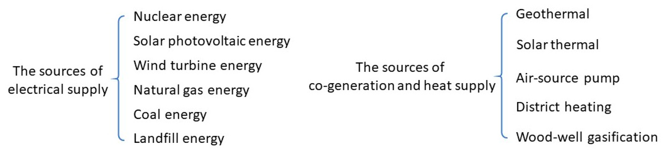
In this section, we present the models of integrated planning of multimodal energy generation plants. We begin by developing the basic risk-neutral model, then propose the risk-averse model based on a coherent risk measure in which we consider multiple objectives (i.e., minimizing total costs and controlling a certain CO2 emission level). In our model, different energy technologies that correspond to various clean energy generation methods are identified and included. The decisions we make are based on the amounts of energy that can be used to provide an electrical and heating supply. Notice that heating demand (e.g., industrial plants, houses, etc.), can be obtained from several sectors, either heating plants or electricity supply, or as a by-product of electricity generation (i.e., co-generation plants). We report the sources of electrical and heating supplies in Figure 1.
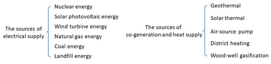
Figure 1.
The sources of electrical and heating supply.
Without a loss of generality, we assume that the region in this paper has access to the electrical and co-generation supplies illustrated in Figure 1, in which we depict sets of possible demand scenarios. Each true demand value is considered to be a realization of the scenario. Under such settings, we should provide a plan to open appropriate plants and allocate energies to meet the specific demands of a region. We illustrate this in Figure 2.
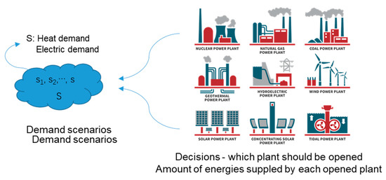
Figure 2.
Illustration of the problem.
To continue to build the model, we first present the notations that will be used through the paper, shown in Table 1.

Table 1.
Notations.
With these notations, we then present the classic model of integrated planning of multimodal energy generation plants.
(A)
s.t.
Model (A) is the basis of our paper, and it aims to minimize the single objective (i.e., total costs), while keeping the total emissions under budget. Constraint (2) enforces that electrical demands should be satisfied. Constraint (3) requires the heating demand to be served. Constraint (4) indicates that only opened plants can supply energy. Constraints (5) and (6) specify the capacity of each plant. Constraint (7) enforces that CO2 emissions should not exceed a certain level. Constraints (8) and (9) define the variables.
Although Model (A) is typically used in practice, we may achieve a more aggressive approach to reducing emissions by minimizing CO2 emissions in the objective function. To do so, we have a bi-objective optimization Model (B):
s.t. (2)–(6), (8)–(9).
Model (B) is a multi-objective stochastic optimization problem. One can obtain a single-objective model by introducing the coefficient of each objective; however, it is pretty hard to obtain the exact value of each coefficient. Therefore, we transform Model (B) into the following equivalent model by defining one of the multi-objectives as a chance constraint:
(B-1)
s.t.
(2)–(6), (8)–(9).
Model (B-1) has the same solution as that of Model (B). The in Constraint (14) is the confidence level or risk level, which can be used to denote the risk preference of a decision maker; is an auxiliary variable. Notice that Constraint (13) derives the main contributions of our risk-averse model from the chance constraint.
As supplementary to above model, we now explain the reason that we assume a case with access to electrical and co-generational sources of power. We aim to consider a more general case where various kinds of generation and demand should be covered. In particular, if the area has no access to co-generation, there is no need to specify and , which leads to the fact that is trivial to the objective function and Constraints (2)–(5). Thus, the model will be totally different without the assumption. However, with the assumption in place, we can regard the case with a single access to be a special case of the current model (i.e., . In addition, in our numerical case, the area does have access to electrical and co-generation sources in practice.
2.2. Risk-Averse Model
Before proposing our risk-averse model, we briefly review the concept of risk measurement. Coherent risk measures have been considered extensively in the literature (for more details, see [25]). Mapping is coherent if it satisfies the following properties for random variables and .
- Monotonicity: If , then ;
- Subadditivity: holds;
- Positive homogeneity: If , then .
- Translation invariance: For , we have .
In this paper, a widely used coherent risk measure (i.e., conditional value-at-risk (CVaR)) is introduced to measure risk of uncertainty. CVaR has been considered extensively in stochastic optimization. Given a risk level , CVaR is formulated as
where . Generally, the quantile is used to denote the risk preference of the decision maker. If , then the decision maker is extremely averse to the uncertainty. Here, we present Proposition 1 to for the computational consideration of a formal formulation of CVaR. Suppose Z is bound, with a support contained in ; in this scenario, we have an equivalent reformulation:
where . This formulation facilitates the calculation of by shrinking the feasible region of η. Considering the outstanding merits of CVaR in leading to a computationally tractable formulation, we will model the problem based on CVaR.
Considering the definition of CVaR and Constraint (14), we are motivated to transform Constraint (14) according to CVaR as
where . Observe that the in Constraint (14) is exactly the in CVaR. Then, introducing a constant which is a user input parameter of risk budget, we have the risk-averse model of the problem:
s.t.
(2)–(6), (8)–(9).
We can linearize the by defining that and
Model (C) has many interesting properties compared to the classic models. We report these properties in following propositions. For ease of notation, we define the solution space as In particular, we let and denote the solution of the risk-neutral Model (B) and risk-averse Model (C), respectively.
Proposition 1.
Given, we haveif.
Proof.
Consider an energy allocation solution with . Let denote the CO2 emissions resulting from , which gives us
and .
Since
and , we have
Therefore, if ,
which means the risk constraint is consistent with Constraint (7), (i.e., the risk-neutral model).
Thus, we have □
Note that if α = 0, then we have a special case of the above proposition, which we report that in the following corollary.
Corollary 1.
For α = 0, we have
Proof.
Based on the definition of CVaR and VaR, we have if α = 0. Then, according to Proposition 1, we can complete the proof. □
Proposition 1 and Corollary 1 indicate that our risk-averse model can be equivalent to the traditional risk-neutral model under certain conditions. Moreover, it implies that the risk-averse model can provide solutions that generate less CO2 than traditional models.
3. Solution Method
Solving Model (C) is challenging because it is an NP-hard problem. Although some commercial software (e.g., CPLEX and Gurobi) can provide exact solutions, they are usually time consuming even for a medium scale problem. Moreover, evaluating the risk measure is somewhat difficult because it might be nonconvex. In this section, we aim to develop an efficient algorithm to solve the model. The idea is that we first form a saddle point problem based on Lagrange duality, and use the primal-dual method learning to update the primal and dual variables simultaneously. The algorithm solves the problem ‘on the fly’ because we dynamically draw samples according to distribution. The algorithm can relax the need for us to know the exact distribution and provide a desirable solution efficiently.
In light of [26], we have
where
and is the set of probability measures of α. Then, Constraint (17) can be approximated by
Here, Introducing Lagrange multipliers for Constraint (18) of Model C, we have the following relaxed optimization problem:
(D)
s.t. (2)–(6), (8)–(9).
Then, we can rewrite Model (D) as
(E)
Model (E) can be rewritten as
(LE)
The Lagrange problem (23) is operated under a scenario set which is indexed by s. With respect to realization s, we have
Then, we can turn to the following sampled Lagrange problem:
We then compute the gradient ascent of primal variables and the gradient descent of dual variable simultaneously, denoted by and . To find the global optimal value, we update primal and dual variables by
where t denotes the index of iterations, and is the step size of updating.
When the iteration reaches the threshold, we stop the algorithm and output the final value. The main procedure of the learning algorithm is reported in the following Table 2.
Table 2.
The primal-dual learning algorithm.
4. Numerical Experiments
In this section, we present a numerical experiment to show the performance of our method. The case is adapted from the energy information report of Yantai and Weihai, a coastal area in China. This is one of China’s seaside resort areas, with tourism and light industry as its main features. During the past decades, large scale migration and industrial expansion have not occurred here. Thus, the total energy demand has been relatively stable. Different power generation technologies exist in the area, such as coal plants, petroleum plants, natural gas plants, nuclear plants, wind turbines, and solar thermal. We collected historical data from 2008 to 2018 on demand, cost, plants, capacity, and emissions (see Table 3, Table 4, Table 5 and Table 6). In Table 3, the first column refers to the total energy demand of the area (381.471 megawatts), which is calculated according to the historical record of electricity consumption of the year 2008. All data used here are extracted from the historical documents, which will be used to verify the resulting optimal planning solution.
Table 3.
Energy demand (in megawatts) of the area from 2008 to 2018.
Table 4.
Energy generation (in megawatts) of the area using different technologies.
Table 5.
Cost of energy (in USD) of different technologies per KWH.
Table 6.
CO2 emissions of different technologies (108 t).
Based on historical data, we generated scenarios based on normal distribution, considering the true value and a 10% variance higher and lower than the true value. We set the risk level as 0.95. All models were computed by Matlab R2015 on a PC with Core i5 7200 8G RAM.
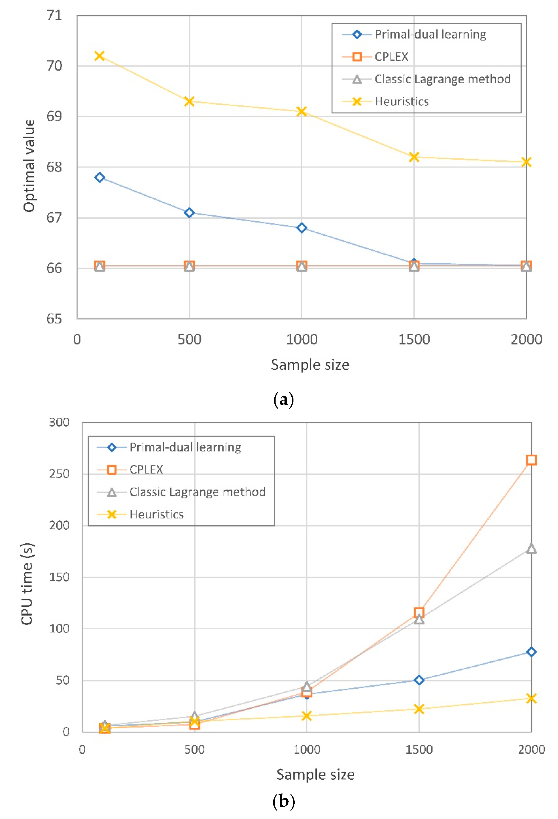
Note that our solution algorithm relaxes the assumption that the exact probability of distribution should be known. Regarding Model (C), we report the convergence and gap in the following figure to show the performance. We used CPLEX, the traditional Lagrange method, and a heuristic algorithm as benchmarks. CPLEX is a well-known commercial software that is able to provide a global optimal solution with known distribution.
As shown in Figure 3, we found that the proposed algorithm in this paper can achieve increasingly accurate optimal values as the sampling size increases. The exact method (i.e., CPLEX) and classic Lagrange method can always provide a global optimal solution without depending on sample size. The gap between our learning method and the exact algorithms becomes sufficiently small when the sampling size reaches 2000. Notice that the benefit we can obtain is that the solution time is quite a bit shorter than the exact algorithms. Although the heuristic method can also provide an efficient solution, the quality of the solution is undesirable (i.e., with a relatively large gap comparing to exact methods). That is to say, our algorithm outperforms exact algorithms in reducing convergence time and the heuristics method in shrinking the gap.
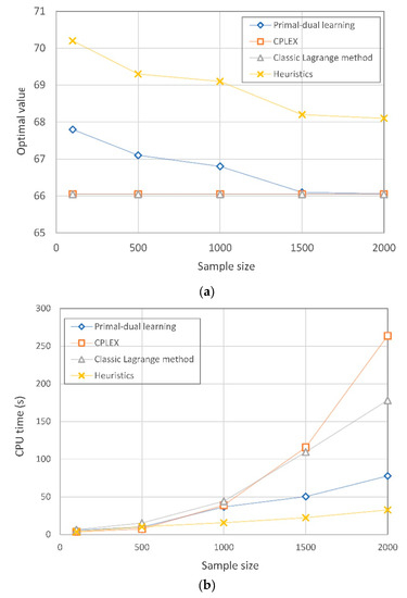
Figure 3.
Performance of the proposed algorithm compared to some benchmarks: (a) optimal value of costs under different sample sizes; (b) CPU time under different sample sizes.
We now turn to show the performance of the risk-averse model compared to the classic risk-neutral model. We first set the risk level as 0.95, and the differences of costs and emissions between the two solutions are shown in Figure 4. We observe that the total costs resulting from the risk-averse model are 8.2% greater than that from the risk-neutral model, while the CO2 of the risk-averse model is 16.8% less than the risk-neutral model. This is because the risk-averse model pays more attention to reducing CO2 emissions using the CVaR constraints, which leads to a result of more clean energy generation facilities being deployed than in the risk-neutral model, as shown in Figure 5. As a result, total costs increase, as clean energy developments are usually more expensive than traditional technologies.
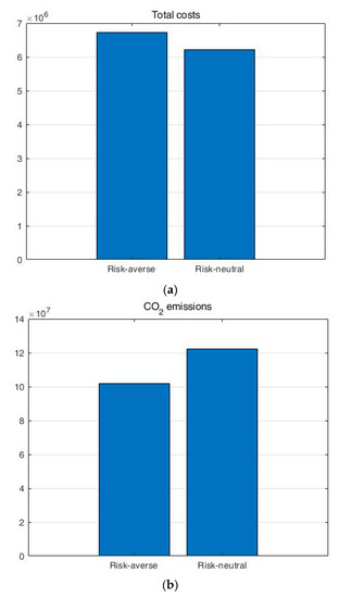
Figure 4.
Total costs and emissions resulting from the risk-averse and risk-neutral models.
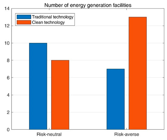
Figure 5.
Number of energy generation facilities built resulting from the risk-averse and risk-neutral model.
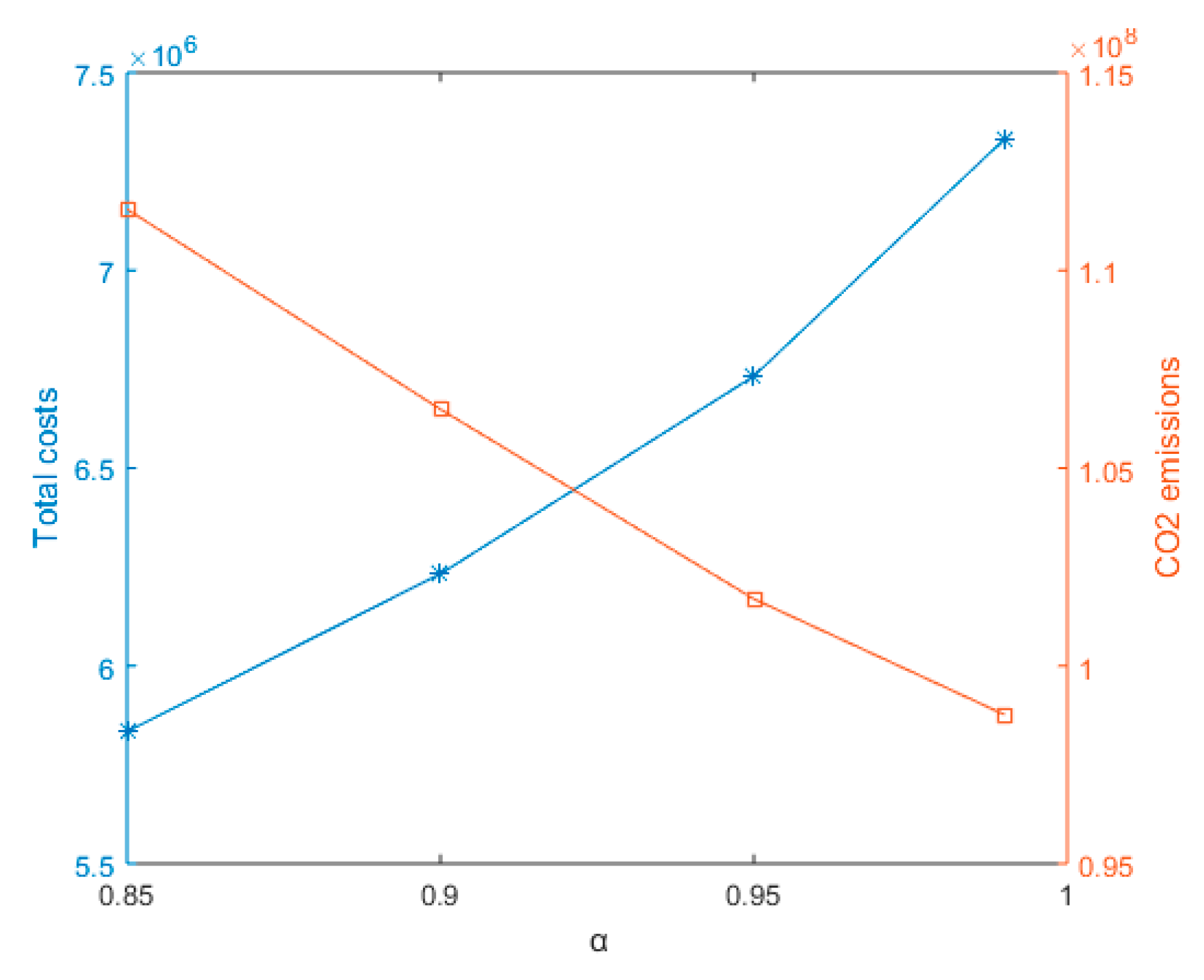
To further see the role of risk-averseness, we perform a sensitivity analysis of the risk level , which indicates the risk preference of decision makers. As shown in Figure 6, with an increasing risk level (i.e., more risk-averse or conservative), the total costs grow while the CO2 emissions reduce. This is because a larger value of α indicates that the determination of the decision maker controlling the emissions is inclined to be stronger, even if the total costs increase as a result.
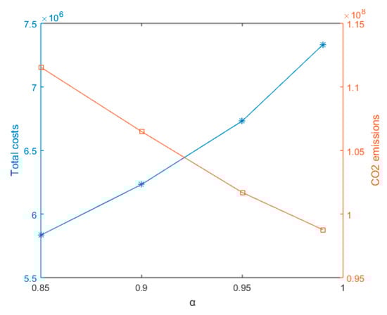
Figure 6.
Sensitivity analysis of risk level to total costs and CO2 emissions.
Thus, the above results imply that the risk-averse model is able to provide solutions that are more friendly to the environment than risk-neutral model. This means that the risk-averse model can contribute more to reducing CO2 emissions.
5. Conclusions
To make a proper planning of multimodal energy generation technologies to meet uncertain demand, we present a risk-averse stochastic programming based on CVaR to minimize total costs control the CO2 emissions below a certain level. We have proven that our risk-averse model can be equivalent to the traditional risk-neutral model under certain conditions. Moreover, this implies that the risk-averse model can provide solutions for generating less CO2 than traditional models. To solve the resulting model efficiently, we developed an approximation algorithm based on the Lagrange primal-dual learning method. A saddle point problem can be formulated based on Lagrange duality, then the primal-dual method learning can be used to update the primal and dual variables simultaneously. We have shown that the algorithm does not need to assume that probability distribution is known a priori, and a desirable gap can be achieved by utilizing historical data.
Due to the complexity of customer and demand, we have not considered the behavior and preferences of customers, which can influence decisions in practice. This will be the direction of our future research.
Author Contributions
Conceptualization and methodology, G.Y.; software, formal analysis, validation, and data curation and writing, X.Z. and X.X.
Funding
This work was partially supported by the National Natural Science Foundation of China (Grant Nos. 71801143, 51805385), the Innovation Method Fund of China (Grant No. 2018IM020200), Shandong Province Natural Science Foundation (ZR2018QG001), and the Fundamental Research Funds of Shandong University (Grant No. 2018JC055). The authors also would like to thank the Young Scholars Program of Shandong University (2018WLJH02) for financial and technical support.
Acknowledgments
Thanks to all the authors of the references who gives us inspiration and help. The authors are grateful to the editors and anonymous reviewers for their valuable comments that improved the quality of this paper.
Conflicts of Interest
The authors declare no conflict of interest.
References
- Alanne, K.; Saari, A. Distributed energy generation and sustainable development. Renew. Sust. Energy Rev. 2006, 10, 539–558. [Google Scholar] [CrossRef]
- Huang, Y.; Yang, K.; Zhang, W.T.; Lee, K.Y. Hierarchical energy management for the multienergy carriers system with different interest bodies. Energies 2018, 11, 2834. [Google Scholar] [CrossRef]
- Lopez-Rey, A.C.-R.S.; Gil-Ortego, R.; Colmenar-Santos, A. Evaluation of supply–demand adaptation of photovoltaic–wind hybrid plants integrated into an urban environment. Energies 2019, 12, 1780. [Google Scholar] [CrossRef]
- Bruno, S.D.G.; La Scala, M.; Meloni, C. A microforecasting module for energy management in residential and tertiary buildings. Energies 2019, 12, 1006. [Google Scholar] [CrossRef]
- Chen, C.; Long, H.L.; Zeng, X.T. Planning a sustainable urban electric power system with considering effects of new energy resources and clean production levels under uncertainty: A case study of tianjin, china. J. Clean. Prod. 2018, 173, 67–81. [Google Scholar] [CrossRef]
- Ebrahimi, S.B. A stochastic multi-objective location-allocation-routing problem for tire supply chain considering sustainability aspects and quantity discounts. J. Clean. Prod. 2018, 198, 704–720. [Google Scholar] [CrossRef]
- Niet, T.; Lyseng, B.; English, J.; Keller, V.; Palmer-Wilson, K.; Moazzen, I.; Robertson, B.; Wild, P.; Rowe, A. Hedging the risk of increased emissions in long term energy planning. Energy Strateg. Rev. 2017, 16, 1–12. [Google Scholar] [CrossRef]
- Chen, Y.Z.; He, L.; Li, J.; Cheng, X.; Lu, H.W. An inexact bi-level simulation-optimization model for conjunctive regional renewable energy planning and air pollution control for electric power generation systems. Appl. Energy 2016, 183, 969–983. [Google Scholar] [CrossRef]
- Xie, Y.L.; Huang, G.H.; Li, W.; Ji, L. Carbon and air pollutants constrained energy planning for clean power generation with a robust optimization model-a case study of jining city, china. Appl. Energy 2014, 136, 150–167. [Google Scholar] [CrossRef]
- Xie, Y.L.; Wang, L.R.; Huang, G.H.; Xia, D.H.; Ji, L. A stochastic inexact robust model for regional energy system management and emission reduction potential analysis-a case study of zibo city, china. Energies 2018, 11, 2108. [Google Scholar] [CrossRef]
- Xie, Y.L.; Xia, D.H.; Ji, L.; Zhou, W.N.; Huang, G.H. An inexact cost-risk balanced model for regional energy structure adjustment management and resources environmental effect analysis—A case study of shandong province, china. Energy 2017, 126, 374–391. [Google Scholar] [CrossRef]
- Ji, L.; Huang, G.H.; Xie, Y.L.; Zhou, Y.; Zhou, J.F. Robust cost-risk tradeoff for day-ahead schedule optimization in residential microgrid system under worst-case conditional value-at risk consideration. Energy 2018, 153, 324–337. [Google Scholar] [CrossRef]
- Lee, S.K.; Mogi, G.; Kim, J.W. Energy technology roadmap for the next 10 years: The case of korea. Energy Policy 2009, 37, 588–596. [Google Scholar] [CrossRef]
- Powell, W.B.; George, A.; Simao, H.; Scott, W.; Lamont, A.; Stewart, J. Smart: A stochastic multiscale model for the analysis of energy resources, technology, and policy. Informs J. Comput. 2012, 24, 665–682. [Google Scholar] [CrossRef]
- Pereira, M.V.F.; Pinto, L.M.V.G. Multi-stage stochastic optimization applied to energy planning. Math Program 1991, 52, 359–375. [Google Scholar] [CrossRef]
- Zhao, J.Y.; Hobbs, B.F.; Pang, J.S. Long-run equilibrium modeling of emissions allowance allocation systems in electric power markets. Oper. Res. 2010, 58, 529–548. [Google Scholar] [CrossRef]
- Simon, C.; Parkinson, N.D. Long-term energy planning with uncertain environmental performance metrics. Appl. Energy 2015, 147, 402–412. [Google Scholar]
- Snyder, L.V. Facility location under uncertainty: A review. IIE Trans. 2006, 38, 537–554. [Google Scholar] [CrossRef]
- Dicorato, M.; Forte, G.; Trovato, M. Environmental-constrained energy planning using energy-efficiency and distributed-generation facilities. Renew. Energy 2008, 33, 1297–1313. [Google Scholar] [CrossRef]
- Muis, Z.A.; Hashim, H.; Manan, Z.A.; Taha, F.M.; Douglas, P.L. Optimal planning of renewable energy-integrated electricity generation schemes with co2 reduction target. Renew. Energy 2010, 35, 2562e2570. [Google Scholar] [CrossRef]
- Modarres, M.; Izadpanahi, E. Aggregate production planning by focusing on energy saving: A robust optimization approach. J. Clean. Prod. 2016, 133, 1074–1085. [Google Scholar] [CrossRef]
- Dellino, G.; Kleijnen, J.P.C.; Meloni, C. Robust optimization in simulation: Taguchi and krige combined. Informs J. Comput. 2012, 24, 471–484. [Google Scholar] [CrossRef]
- Yu, G.D.; Haskell, W.B.; Liu, Y. Resilient facility location against the risk of disruptions. Transport Res. B Methodol. 2017, 104, 82–105. [Google Scholar] [CrossRef]
- Ben-Tal, A.; Nemirovski, A. Robust optimization - methodology and applications. Math Program 2002, 92, 453–480. [Google Scholar] [CrossRef]
- Yu, G.D.; Li, F.; Yang, Y. Robust supply chain networks design and ambiguous risk preferences. Int. J. Prod. Res. 2017, 55, 1168–1182. [Google Scholar] [CrossRef]
- Shapiro, A. On kusuoka representation of law invariant risk measures. Math. Oper. Res. 2013, 38, 142–152. [Google Scholar] [CrossRef]


© 2019 by the authors. Licensee MDPI, Basel, Switzerland. This article is an open access article distributed under the terms and conditions of the Creative Commons Attribution (CC BY) license (http://creativecommons.org/licenses/by/4.0/).