1. Introduction
The characteristics of the motor itself are mainly tested by connecting mechanical components, designed for mass or friction load, to the motor shaft [
1]. On the other hand, the test should be performed under various load conditions if the motor is developed for high reliability applications such as electric vehicles [
2,
3], wind power generators [
4], aircraft [
5], etc. In this case, it is customary to test the motor and its driving circuits together by connecting them to another electric machine, usually called a programmable dynamometer, which produces mechanical torque that is supposed to act on the motor as load torque in the real operation.
In recent research, several methods for the dynamic load emulation were proposed, in which the torque of the programmable dynamometer was determined by some closed-loop algorithms so that the dynamics of the emulator became that of a desired one. One of early results given in [
6] employed the inverse model of the system. The structure proposed in [
6] was simple and easy to understand, so that it is convenient to implement in various applications. In [
4], the authors developed an algorithm to emulate the effect of an inertia using a hardware-in-the-loop wind turbine simulator. Nonlinear and possibly discontinuous load torques were emulated in [
7]. The performance of these approaches was limited. The approach in [
6] was sensitive to measurement noises, since it involved the inverse of a strictly proper transfer function, and it is not possible to emulate an inertia that is much larger than the actual inertia of the test-rig [
8]. In [
8], the authors proposed an alternative controller, called feedforward-tracking, where a feedforward term was added to compensate the motor torque, and the load emulation was performed by an additional speed control loop. This controller has been well accepted in the industry, and its performance has been verified through various experimental results, e.g., emulation of a flexible-shaft [
9], emulation of the model by applying the parametric system identification method [
5], and some experiments using industrial drives [
10]. It is noted that in the above approaches, the effect of plant uncertainties on system stability and performance were not explicitly addressed.
In this paper, a disturbance-observer (DOB)-based emulation scheme is presented. A preliminary result has been reported in [
11], where the basic idea was introduced. DOB is a robust output feedback controller and has been successfully employed to compensate the external disturbances and plant uncertainties in many real applications such as robust servo control [
12] and robust track-following of an optical disk drive [
13]. See the survey [
14] for various DOB-based controller and related methods. Roughly speaking, the dynamic inverse of the nominal model of the plant is used to estimate the input combined with the disturbance, and the disturbance is estimated by subtracting the input from the proceeding signal. In fact, the resulting estimate of disturbance is different from the actual external disturbance due to plant uncertainty, and thus, it is the combined effect of plant uncertainty and the external disturbance. One of the key benefits of DOB is that it can recover the performance of a nominal closed-loop system that is composed of the nominal plant and the controller designed for the nominal system [
15,
16]. We call this property
nominal performance recovery.
The nominal performance recovery property of DOB is exploited to obtain a robust emulation scheme, and the key idea is to regard the dynamics to be emulated (e.g., a mechanical system with a desired inertia and damping) as the nominal plant in the DOB scheme. This new idea enables us to successfully address the emulation problem considering the plant uncertainty. We emphasize that this robustness against plant uncertainty in the emulation problem makes our result different from previous emulation approaches mentioned above. Another important contribution is that the range of emulation parameters is wider than previous results, and a rigorous stability analysis in the state space is carried out, which was not taken into account in previous research. Note that this time-domain analysis helps us to consider the nonlinear load emulation. Finally, the efficacy of the proposed method is also verified through various experiments for both linear and nonlinear loads.
The rest of this paper is organized as follows.
Section 2 formulates the problem in this paper.
Section 3 presents the main idea of the proposed method to emulate the mechanical load and the load torque. In this section, the performance of the proposed method is guaranteed by a rigorous stability analysis. In
Section 4, the proposed method is verified by some experiments using two electrical machines. Finally, some concluding remarks are shown in
Section 5.
2. Problem Formulation
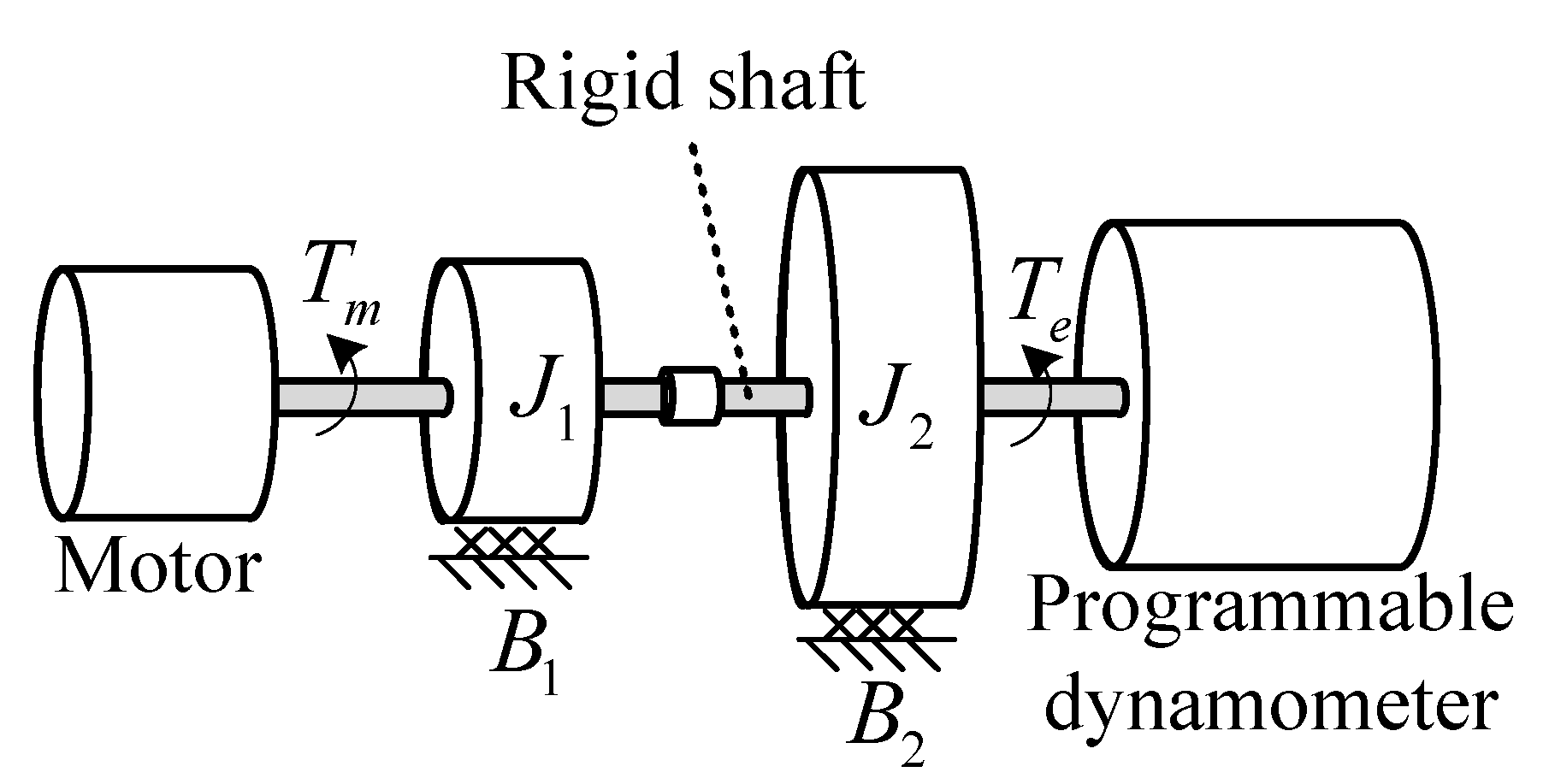
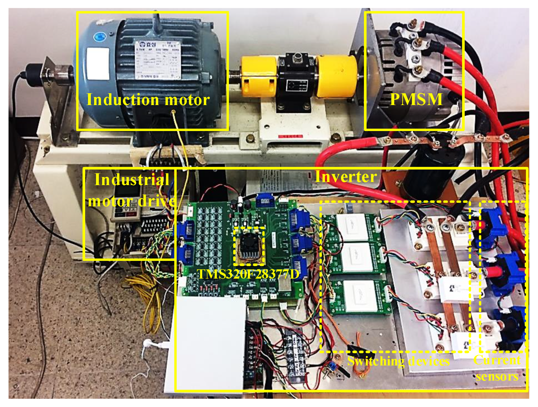
We consider a motor test system, shown in
Figure 1, which is composed of an electric motor to be tested and another electric machine, called a programmable dynamometer.
Two electrical machines in the system are connected by a rigid shaft, and thus, the dynamics is given by:
where
is the lumped inertia of the shaft, which includes the inertia of the driving motor and that of the load machine,
is the friction coefficient, which is also a lumped parameter,
is the electrical torque generated by the motor under test,
is the torque from the dynamometer,
is the rotating speed of the shaft, and
d is the disturbance torque.
Suppose that the motor under test is connected to a desired mechanical load with inertia
and friction
. In this case, the dynamics becomes:
where
and
are the rotating speed and the load torque of the desired dynamics to emulate. The control objective is to manipulate
so that
of (
1) follows
of (
2) as close as possible. The transfer functions of (
1) and (
2) are derived as follows:
where:
In many previous research works, the controllers were designed in the frequency-domain considering the transfer functions (4). In [
6], the dynamometer torque was generated as
in order to correct the speed response
of (
4a) into (
4b), and [
8] proposed to use
where
with a design parameter
. Both [
6,
8] neglected the disturbance torque and load torque and required the knowledge of the parameters
J and
B, but the effects of the parameter uncertainties were not addressed in detail. Note that the performance of the controller was degraded by the parameter uncertainties in many cases.
Unlike the earlier works, the disturbance/load torque will be taken into account, and it is assumed that the exact values of the parameter J and B are unknown. Instead, the following assumptions were made.
Assumption 1. It is assumed that the plant parameters J and B are uncertain, but belong to the following bounded sets: Assumption 2. The torques , and the external disturbance d are twice differentiable and bounded, i.e., there exists , , with known constants , , and , respectively.
In the following sections, a new emulation method for generating the dynamometer torque will be proposed with its performance/stability analysis.
3. Robust Load Emulation Controller: Theory
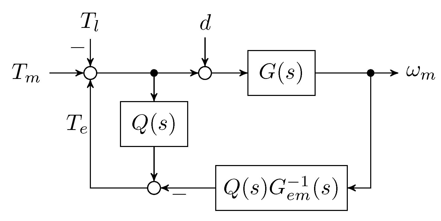
Figure 2 illustrates the application of the conventional DOB to load emulation, which is similar to the servo-control scheme of [
12]. Compared with [
12], the figure has some distinctive features such that the load torque
is added, and the nominal model of the plant is replaced by the emulating dynamics
.
From this figure, the closed-loop system can be written as:
where
is the low pass filter with unity DC gain (
), called the Q-filter in the conventional DOB structure. It can be observed that the closed-loop system (
5) will behave like the desired emulation dynamics (
3b) in the low frequency range.
A state-space emulation method that can be expressed as follows will be developed:
where
q is the state of the controller and
and
are functions to be designed. Thus, it is required to redraw
Figure 2 so that the
can be made from
,
, and
is shown clearly as per the following subsection.
3.1. Disturbance Observer-Based Emulation Method
From
Figure 2, the dynamometer torque is generated by:
where the Q-filters are chosen as
(This is a Type-I Q-filter in [
12]. Since the proposed emulation method is based on DOB (
Figure 2), the higher-order Q-filters are also available in order to improve the emulating performance.) with design parameters
in this paper. Note that there is an algebraic loop of
in (
7). Thus, it can be rewritten as:
Let
, then a state-space realization of (
8) is obtained as follows:
which could be considered as the implementations of
(
6a) and
(
6b).
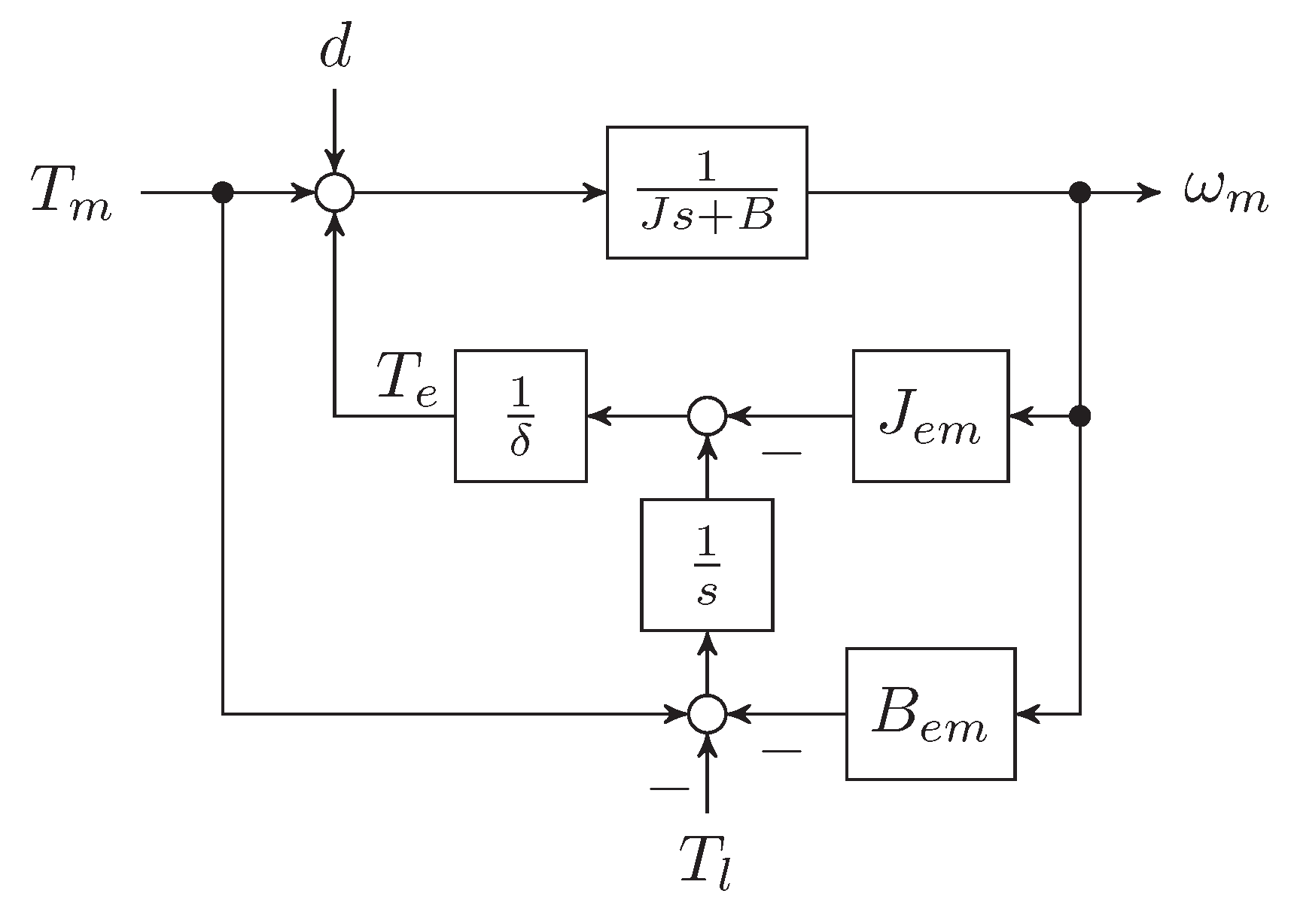
One can see that (9) can be drawn as
Figure 3, and it is a particular implementation of
Figure 2. It will be proven later that the performance of this structure is guaranteed as:
where the trajectory of the actual system (
1) follows the desired emulation dynamics (
2) within a bound
.
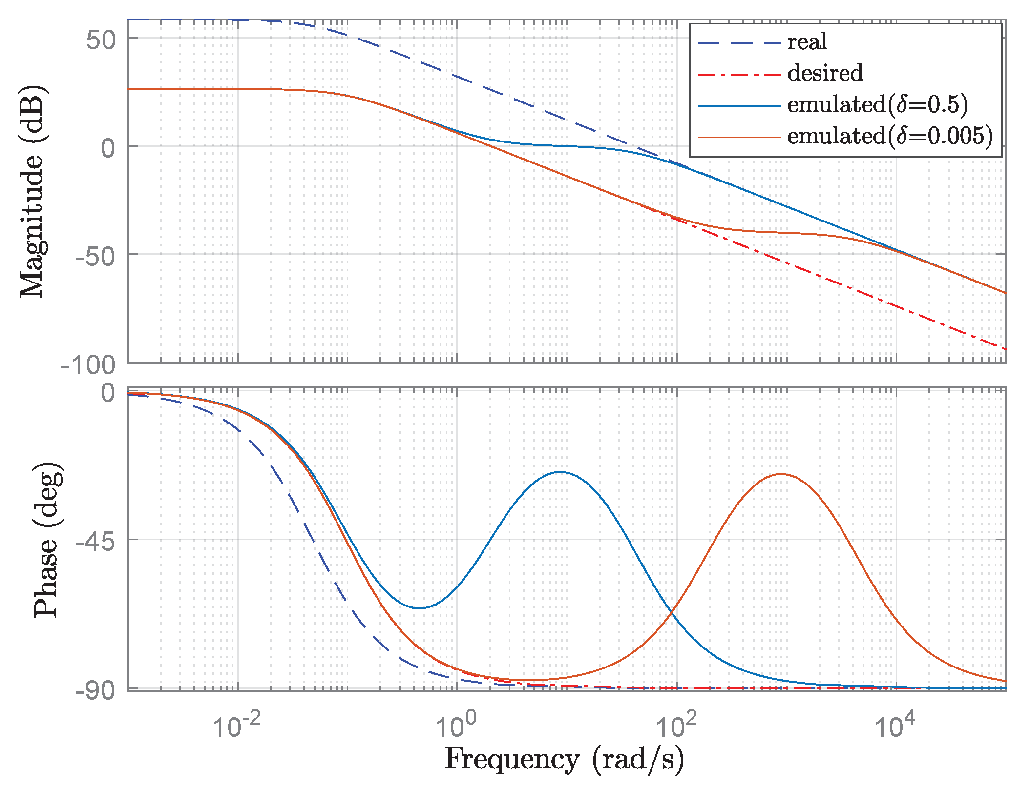
Figure 4 shows the Bode diagram of the real dynamics (4a), desired dynamics (4b), and emulated dynamics (5) for different
’s. In the diagram, it is clear that the frequency response of the emulated dynamics is close to that of the desired dynamics in the low-frequency range and that this frequency range is increased as a smaller
is used.
3.2. Performance Analysis
This section presents the emulating performance of the proposed method based on the singular perturbation theory [
17].
Lemma 1. There exists a such that the closed-loop system (1) and (9) is exponentially stable. Proof. Let us denote
as
for convenience. It is a matter of simple algebra to show that the closed-loop system becomes:
This is the linear system (with respect to the inputs
,
, and
d, respectively.) whose system matrix is given by:
and this matrix is Hurwitz for some
. This completes the proof. □
In Lemma 1, the closed-loop system (
11a), (
11b) is written in the standard singular perturbation form [
17]. Based on the singular perturbation theory, the closed-loop system is divided by the slow variable (
) and the fast variable (
) with the time-separation parameter
. For sufficiently small
, the slow variable is frozen, while the fast variable
converges to its equilibrium, namely
:
Suppose that the fast variable has converged (
); the slow variable behaves like the the desired emulation dynamics (
2):
under consideration in this paper. This kind of approach was also shown in [
11], but the stability analysis was limited by perfect time scale separation, in which the goal (
2) was achieved by assuming arbitrary small
.
Remark 1. In recent DOB approaches [15,16], the standard singular perturbation form was obtained by some coordinate transforms. On the other hand, no additional procedure is required in the proposed method due to the simple structure (9). Now, the realistic condition (
) is considered in this paper. To evaluate the emulating performance, the emulating error
is taken into account with the the fast variable by the coordinate change
,
In (
14b),
is directly computed from (
13) as follows:
where
,
, and
, respectively. It can be easily shown that the response of the emulating error is determined by the stable transfer function:
which is computed from (14) and (
15). In (
16), the input signal
is bounded (see Lemma 2 for more detail) under the assumptions in this paper; it follows that there exists a positive constant
, the emulating error is bounded by
.
Lemma 2. Under Assumptions 1–2, the conservative bound of the input signal can be computed by:where the bound is obtained using the knowledge of the desired emulation dynamics (2), and the constants are computed by: The proof is omitted, since it is obvious.
Finally, the emulating performance of the proposed method is guaranteed by the time-domain analysis, in which the Lyapunov stability analysis of the proposed method is shown by the following theorem.
Theorem 1. For the given desired bound , there exists a constant such that for any , the trajectory of the closed-loop system (14) and (15) satisfies (10). Proof. The dynamics
is compactly rewritten by:
Consider a Lyapunov function candidate:
with the positive constants
and
to be determined. Then,
where:
and
is a positive constant from the Young’s inequality.
From (
18), the global exponential stability of the origin of the unforced system will be investigated with
. By choosing
,
, and
such that:
this guarantees the exponential stability of the origin for any
. Now, the input
is allowed to obtain
where
. By the comparison lemma, we have:
from which it follows that:
Since
is an arbitrary constant, (
20) completes the proof. In other words, for a given
, there exists
such that for any
satisfying
, it holds that:
□
The analysis of this paper implies that sufficiently small is required to guarantee the desired performance . One can obtain by computing the conservative bounds of the signals or via repeated experiments, as shown in the next section.
4. Experimental Result
In this section, experimental results are provided to show that: (1) the proposed method emulates a wide range of the linear dynamic loads, and it also compensates the effects of the disturbance torque d; (2) the emulation of the desired dynamics can be performed in the presence of various load torques .
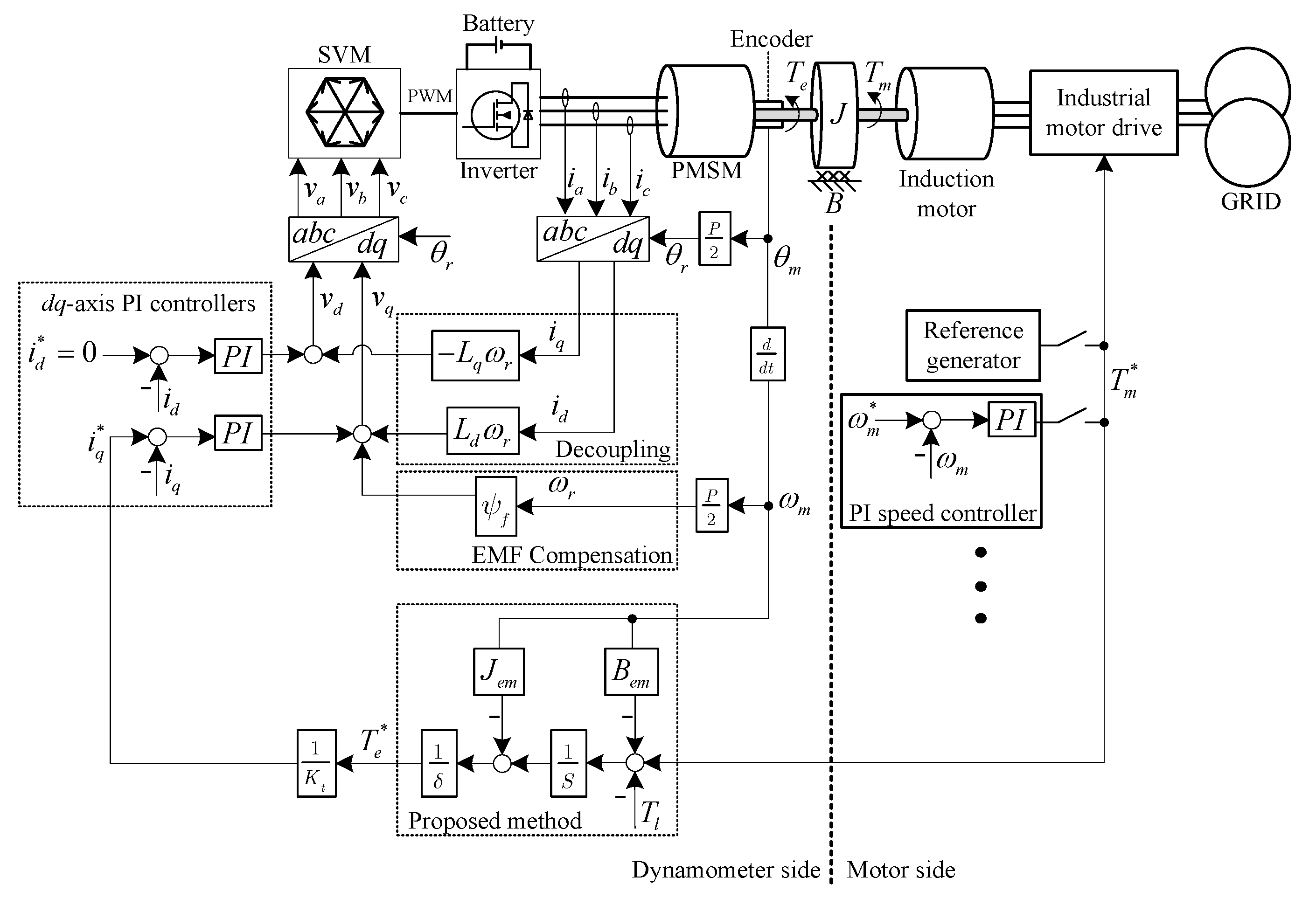
Figure 5 and
Figure 6 show the experimental setup and its block diagram, respectively, to evaluate the performance of the proposed method (
Figure 3). The electrical parameters of the PMSM and the induction motor are described in
Table 1. The proposed method was implemented in a microprocessor, TMS320f28377D with a 200-MHz clock frequency. Three-phase currents (
) were measured by the current sensors, while three-phase voltages (
,
,
) were applied to the PMSM through the switching devices with the switching frequency
kHz and the DC-link voltage
V. The PI-gains of the dq-axis current controllers were chosen as
(or
) and
where
denotes the desired bandwidth of the current controllers [
18]. The rotating speed of the shaft was computed by the numerical differentiation:
where the shaft angle
was measured by a sin/cos encoder in order to alleviate some problems related to the numerical differentiation, since this provided significantly higher resolution of the measurement than conventional optical encoders. All measurements were monitored by a laptop every
ms using the CAN protocol.
4.1. Implementation of the Proposed Method with the Electrical Machine
In the motor side of
Figure 6, the induction motor was used to generate
with a commercial motor drive (Varispeed G7, YASKAWA), where the reference of
is denoted by
. Various operations were carried out using the commercial motor drive to test the performance of the load emulator. In the dynamometer side, the PMSM was used to generate
following the output of the proposed disturbance-observer
. The emulation was performed by a cascade control scheme, i.e., the proposed disturbance-observer (
Figure 3) generated
in the outer-loop, and the conventional field-oriented current control formed the inner-loop. In all experiments, the rotating speed and the torques were measured, and the results were compared with the response of the desired dynamics obtained by the numerical simulation. The measurement
followed the simulation result
, if the emulation was successfully performed by the proposed method.
In
Figure 6, the proposed method was applied under the following assumptions:
The tracking dynamics of the -axis current controllers and the torque controller in the industrial motor drive were negligible due to their fast responses; thus, it was assumed that , , and , respectively.
Since was controlled by the d-axis controller, the torque was developed by the relation where is the well-known torque constant.
These kinds of assumptions have been adopted by many previous researchers.
4.2. Experimental Results: Linear Loads
Figure 7 shows the responses when the sinusoidal reference
Nm was applied to the motor. In the experiments, the desired dynamic loads were chosen as
,
Nms/rad, and
, respectively. The design parameter
of the controller was changed to demonstrate the performance. In
Figure 7a, it can be observed that the emulating error was decreased as
became smaller, while
Figure 7b shows that the disturbance torque
d was compensated by the dynamometer. Since (
13) holds
in this case, one can choose the value of
by similar procedures as shown in
Figure 7. For the rest of experiments, we fixed
. This value was chosen to compromise between the tracking accuracy and the smoothness of
. Note that in the case with
, we had more accurate tracking error (
Figure 7b), while in the case with
, we had a smoother profile in
.
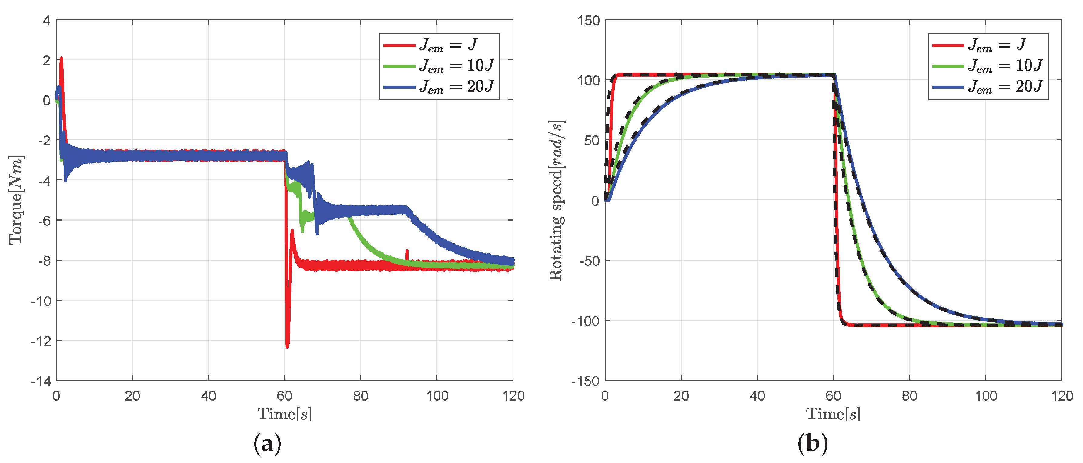
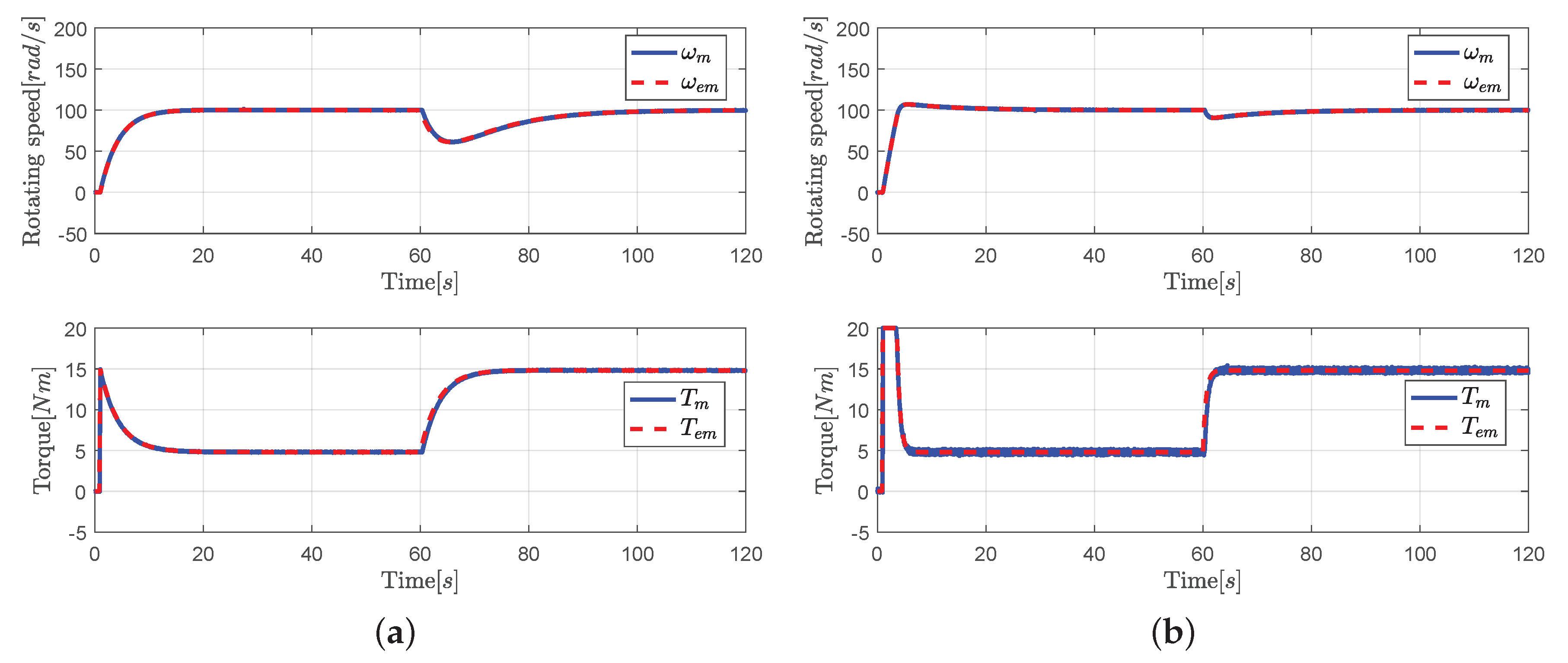
Remark 2. In fact, the disturbance torque d is unknown in practice. The proposed method compensates the total disturbance (13) including the estimation of the disturbance, as discussed in earlier. Figure 8 shows the responses with respect to various dynamic loads
to emulate. The step input
Nm was applied to the motor, where
denotes the unit step input (
if
, otherwise it is zero). At 60 s, the load torque
Nm to emulate was also applied. In the simulation, the emulation error
was less than
when the response of the desired emulation dynamics (
2) was relatively fast with small
. The emulation error became smaller in the case of larger
.
Remark 3. In many previous research works, the experiments were performed under relatively limited conditions compared to the results in this paper, e.g., for the linear load [8,9], for the nonlinear loads [19], and with the industrial motor drives (SIEMENS) using HIL devices [10], respectively. Figure 9 shows the case when the motor side was driven by a conventional PI-type speed controller:
where
and
are the PI gains of the controller; the reference speed and the load torque are given by
rad/s and
Nm in this experiment. The desired dynamic loads were chosen as
and
. Note that the motor torque was developed by the closed-loop controller (
21), unlike previous experiments; thus, the simulation results to be compared were also given by closed-loop system:
where
and
correspond to the measurement
and
. In addition, the saturation function was added to limit the motor torque within
Nm. In the figure, it can be observed that both the torque and the rotating speed of the motor-side were emulated with very small errors (
and
).
4.3. Experimental Results: Nonlinear Loads
In this experiment, the performance of the proposed method was verified by emulating a nonlinear friction load:
where
m is the mass,
is the velocity of the mass,
is the conversion ratio between the velocity
and the rotational speed
,
g is the gravitational acceleration,
is the slip velocity, and
is a nonlinear function based on Burkhardt model with the coefficients
, respectively [
3]. Now, the proposed method corrected the actual dynamics (
1) of the test-rig (
Figure 6) into the desired dynamics (
24a), while the load torque
was generated by the dynamic model (
24b) and (
24c), which was also implemented in the dynamometer side. In addition, the motor torque was applied by a nonlinear controller:
where
is the desired slip velocity,
and
are the design parameters of the controller,
denotes the sign of the input signal (1 or
), and
represents the saturation function to limit the motor torque within
Nm.
Remark 4. The dynamics (24) represents the dynamic behavior of a single wheel in a vehicle under the hard braking condition [3], i.e., is called adhesion force, which is determined by the slip velocity of the vehicle λ. The controller (25) is also known as the bang-bang controller in order to prevent skidding of the vehicle. One can easily test the behavior of the closed-loop system (24) and (25) by using the simulation model in MATLAB/Simulink [20]. Figure 10 shows the experimental results when the parameters of the desired emulating dynamics (24) were chosen as
kg,
,
,
,
,
, and
, respectively. The initial conditions of the rotating speeds were given by
rad/s. The simulation results to be compared are denoted by
,
and
(which correspond to the measurements
,
, and
by emulating (24)), respectively. In the figures, the responses of the torques are slightly different
Nm with the phase difference, while the emulating error
is less than 5 rad/s. The emulating performance degraded in this experiment, because the motor torque was significantly varied by using the sign function (
25).


