Research and Application of a Hybrid Wind Energy Forecasting System Based on Data Processing and an Optimized Extreme Learning Machine

Abstract

Accurate wind speed forecasting plays a significant role for grid operators and the use of wind energy, which helps meet increasing energy needs and improve the energy structure. However, choosing an accurate forecasting system is a challenging task. Many studies have been carried out in recent years, but unfortunately, these studies ignore the importance of data preprocessing and the influence of numerous missing values, leading to poor forecasting performance. In this paper, a hybrid forecasting system based on data preprocessing and an Extreme Learning Machine optimized by the cuckoo algorithm is proposed, which can overcome the limitations of the single ELM model. In the system, the standard genetic algorithm is added to reduce the dimensions of the input and utilize the time series model for error correction by focusing on the optimized extreme learning machine model. And according to screened results, the 5% fractile and 95% fractile are applied to compose the upper and lower bounds of the confidence interval, respectively. The assessment results indicate that the hybrid system successfully overcomes some limitations of the single Extreme Learning Machine model and traditional BP and Mycielski models and can be an effective tool compared to traditional forecasting models.

1. Introduction

At present, the increasing energy demand, security of the energy supply and reduction of emissions are the most difficult challenges that need to be address urgently for the whole world [1]. Energy consumption, which accounts for 60% of global greenhouse gas emissions, has already contributed to climate change [2]. How best to stop climate change and global warming while still satisfying the world’s energy consumption, without impairing the global economy, is an essential problem for every country [3]. There is no doubt that renewable energy is an appropriate way.

In renewables, wind power technology is regarded as the most mature of the new technologies today, with the potential to cover more than 20% of the global electricity demand by 2050 [4]. By the end of 2015, the worldwide total cumulative installed wind capacity had reached about 432,680 MW [5]. Wind touches our life in countless ways all the time. Thus, research on wind power production can be taken as an illustrative case for renewable energy.

Wind energy is of great significance in many countries’ energy structures and has received a large amount of attention as a type of renewable energy. However, many problems connected with wind power generation have arisen, which seriously restrict the development of the wind power [6]. Due to the intermittency and stochastic fluctuations of wind, wind speed forecasting is one of those problems. If the wind speed forecasting error were to decrease by 1%, the operating costs would decrease by 10 million pounds [7]. In recent years, a large amount of research has been directed toward the improvement of accurate and reliable wind speed forecasting models. Many different approaches have been proposed and developed at home and abroad. These forecasting methods can be classified into four main categories: physical models, statistical models, artificial intelligence models and hybrid models.

Physical models, which are suitable for long-term wind speed forecasting, consider not only historical data, but also make use of physical parameters, including temperature, density, speed, and topography information [8]. However, physical methods always cost a great deal of computing time and thus are not suitable for wind speed forecasting. In physical models, the numerical weather prediction (NWP) model has been widely employed. Lynch et al. [9] presented a simplified forecasting method, deriving the Kalman Filter Covariance Matrices from a NWP model. The adoption of KF technique can successfully extract results that better reflect local conditions. Landberg [10] studied the performance of different models for wind speed forecasting, including the NWP and an artificial neural network (ANN), and so on. However, models adopting the physical methods are time and resources consuming. Besides, these methods are more suitable for weather forecasting rather than wind speed forecast.

Statistical methods always build mathematical and statistical models to forecast future wind speeds [11]. Common statistical techniques include Auto-Regressive Moving Average, Autoregressive Integrated Moving Average, fractional ARIMA, exponential smoothing and grey prediction. They are built based on the relationship between each variable by mathematical statistics to describe the potential correlations from history data sampling for wind speed forecasting [12]. Schlink and Tezlaff applied AR for wind speed forecasting task at an airport [13,14], and the results showed that the width of intervals produced by AR were narrower than the intervals generated by the persistence model [14]. Torres et al. [15] applied standardized data and ARMA model to forecast wind speed series in Navarre and presented a comparison between the model results and meteorological forecasts. The results show that ARMA model has a good effect. Taylor et al. [16] applied an ARFIMA-generalized autoregressive conditional heteroskedasticity (GARCH) model to forecast hourly wind speed series and presented a comparison between the model results and meteorological forecasts. However, statistical models are based on the assumption that there are linear patterns among time series, so they are unfit for accurately forecasting the complex and nonlinear electrical power system series [17].

The intelligent methods do the wind speed forecasting by adopting the artificial intelligence theories or evolutionary algorithms. Artificial intelligence prediction models are mainly focused on artificial neural networks (ANNs), including the back propagation neural network (BPNN), radial basis function neural network (RBF), Elman neural network (ENN) and wavelet neural network (WNN). Younes and Mohammad [18] employed ANN for predicting the temporal dimension of wind speed at one-hour time interval, as a short-term wind speed prediction. Adil et al. [19] developed wind speed time series model using a Nonlinear Autoregressive Neural Network (NARNN). In the study, historical wind data is taken for training and testing the developed NARNN. The evaluation criteria include several standard performance indices namely Mean Absolute error (MAE), Symmetric Mean Absolute Percentage error (SMAPE) and Root Mean Square error (RMSE). Liu et al. [20] proposed a wind speed prediction based on the Elman neural networks (ENN) and the Secondary Decomposition Algorithm (SDA) which combines the Wavelet Packet Decomposition (WPD) and the Fast Ensemble Empirical Mode Decomposition (FEEMD). Maatallah et al. [21] put forward an artificial intelligent wind speed forecasting model optimized by the HM and the AR approach, which suited for a short-term horizon. The model simulations results showed that this hybrid intelligent model outperformed both of the ARIMA model and the ANN model. Accordingly, development of hybrid models should be taken into consideration, which is deemed as an effective method to utilize the advantages of each approach and obtain higher forecasting accuracy.

The combination forecast theory was first proposed by Bates and Granger in 1969 [22]. Since the 1970s, the study of combined forecast models has been a popular field in wind speed forecasting [23,24]. In consideration of high accuracy and stability, the application of multi-objective optimization algorithms in the forecasting fields is worth studying [25]. Xiao et al. [26] reviewed and classified the combined wind speed forecasting models, then proposed the NNCT (no negative constraint theory) combination model and the artificial intelligence algorithm combination model. do Nascimento Camelo et al. [27] studied two innovative hybrid methodologies capable of performing short and long term wind speed predictions. The one is ARIMAX-ANN hybrid model and the other is Holt-Winters-ANN hybrid model. Their simulations showed that the two hybrid models can offer effective wind speed forecasting results. A wind speed forecasting method based on improved empirical mode decomposition (EMD) and GA-BP neural network is proposed by Wang et al. [28]. The simulation with MATLAB shows that the proposed method can improve the forecasting accuracy and computational efficiency.

Although previous studies have achieved satisfactory forecasting results, most of them analyze relatively complete data sets and rarely mention the specific process of data preprocessing. For data with more missing values, many current methods have limitations and cannot be used directly to promote. For example, the EMD method is limited based on missing values. Moreover, one thing to note for wavelet decomposition is the processing of the boundary point, and when adding new data, part reconstructed decomposition coefficient would change, which may require a new training model and thus increase the operation time.

Based on the analysis above, a wind speed forecasting system which can increase forecasting accuracy effectively was developed in the paper. The system can be divided into data preprocessing, algorithm optimization, wind speed forecasting and accuracy evaluation modules.

Our contributions are described as follows:

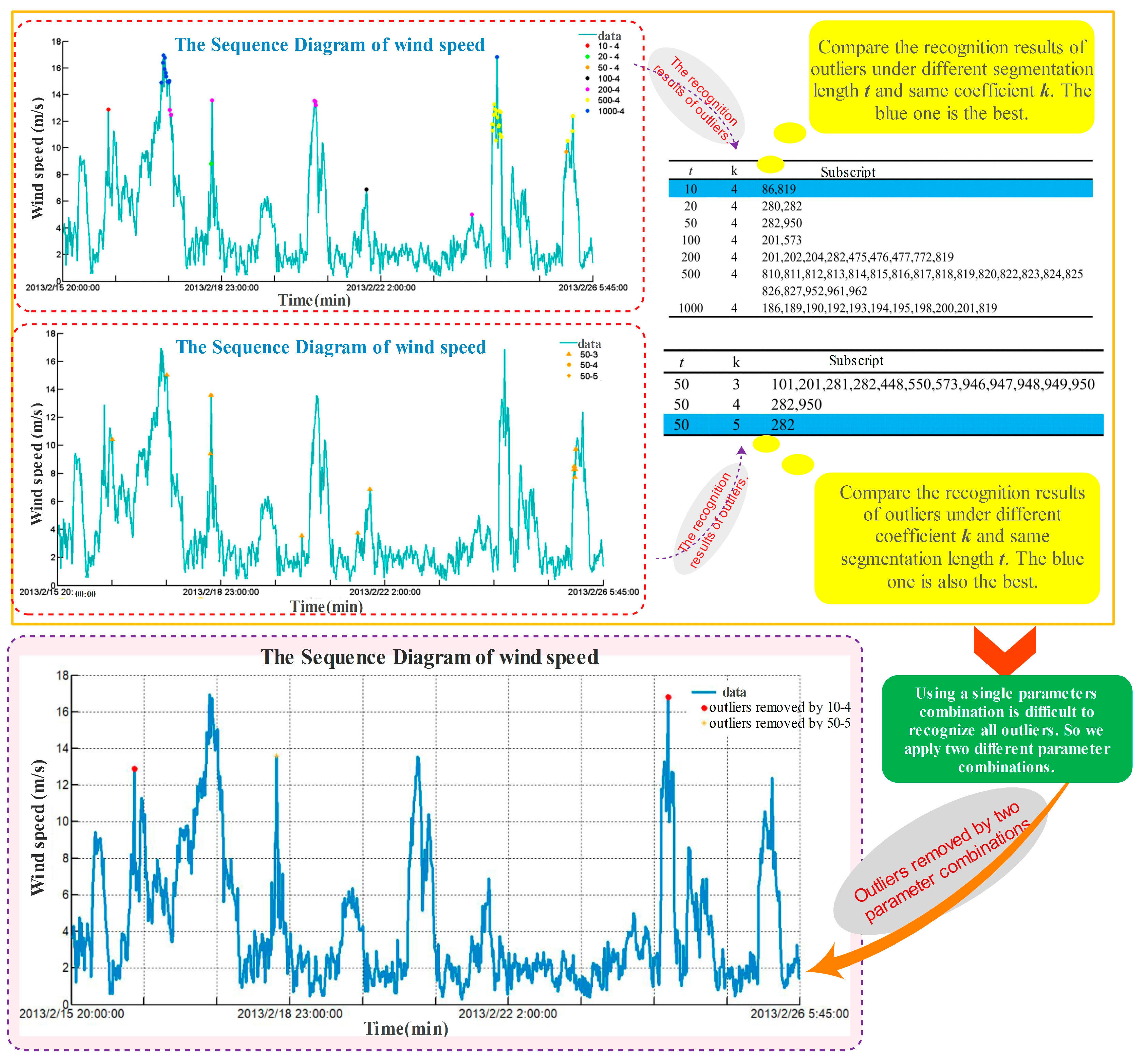
• In the data preprocessing module, the Dynamic absolute mean value method and Cubic Spline interpolation is employed to eliminate outliers and process the missing data, respectively. The Dynamic absolute mean value method can define the scope of outliers effectively by setting the value of the segmentation length and the coefficient. Cubic Spline interpolation not only can overcome the defects in high-order polynomial interpolation but also can guarantee a certain smoothness of piecewise interpolation.
• In the algorithm optimization module, the ELM algorithm is optimized by the Cuckoo Search algorithm. The Cuckoo Search algorithm is abstracted to solve various optimization problems by simulating the nest parasitic behavior in the natural world. In the paper, it is used to optimize the initial weight of ELM and then increase the forecasting accuracy.
• In the wind speed forecasting module, an innovative hybrid system which successfully takes advantages of CSELM algorithm and SGA algorithm is proposed. Then, according to this, we conduct an empirical analysis on the wind speed of Dangjin Mountain located in Akesai, China. The combined system can provide more accurate and stable wind speed forecasting results compared with traditional forecasting models.
• A more scientific and comprehensive evaluation is conducted to estimate the performance of the developed forecasting system in this paper. The evaluation system contains the performance of the whole research process including data preprocessing, optimized algorithm and empirical forecasting results.

The reminder of the paper is organized as follows: Section 2 introduces the algorithms for the outliers and the imputation method for missing data. Attempting to overcome the low forecasting accuracy of the single ELM method, this article proposes a prediction model that optimizes the initial weight of ELM by using Cuckoo Search. Section 3 filters the input and output matrix established by SGA, calibrates the forecasting error using the sliding ARMA process and estimates the upper limit and lower limit of the prediction point’s confidence interval based on historical samples. Finally, Section 4 concludes the paper.

2. Data Preprocessing and Proposed CS-ELM Model

The section can be primarily divided into two parts. The first part introduces the algorithms for the outliers and the imputation method for missing data. Attempting to overcome the low forecasting accuracy of the single ELM model, this second part proposes a prediction model that optimizes the initial weight of ELM via the usage of Cuckoo Search and contrast the prediction results obtained from BP and Mycielski.

2.1. Multiple Patterns

This part introduces the Dynamic absolute mean value method, Cubic Spline interpolation function, Extreme Learning Machine and Cuckoo Optimization Algorithm in turn. Dynamic absolute mean value method is used to process outliers and Cubic Spline interpolation is applied for missing data interpolation. Extreme Learning Machine is a method, which is applied to forecast based on the processed data. Targeting at the poor forecasting accuracy of single ELM model, ELM model is optimized by Cuckoo Search in the paper.

2.1.1. Dynamic Absolute Mean Value Method

Let $x_1,x_2,x_3,\cdots ,x_n$ be an evenly spaced discrete sequence that is segmented at a fixed length $\tau (\tau <n)$. This part focuses on the first segmented sequence and calculates as follows:

Definition 1.

Calculate the mean value:

$$\overline{x}=\frac{1}{\tau }\left(x_1+x_2+x_3+\cdots +x_{\tau }\right)$$

(1)

and write the new sequence as:

$$x_1^{\prime }=x_1-\overline{x},x_2^{\prime }=x_2-\overline{x},\cdots ,x_{\tau }^{\prime }=x_{\tau }-\overline{x}$$

(2)

Definition 2.

Calculate the absolute mean value of the new sequence:

$$\overline{x^{\prime }}=\frac{1}{\tau }\left|x_1^{\prime }+x_2^{\prime }+\cdots +x_{\tau }^{\prime }\right|$$

(3)

iterate over the new sequence $x_1^{\prime },x_2^{\prime },\cdots ,x_{\tau }^{\prime }$ and mark the value that is larger than the threshold $k·\overline{x^{\prime }}$. For $x_i^{\prime }$ such that $x_i^{\prime }>k·\overline{x^{\prime }}$, $x_i^{\prime }$ is generally the bad data for $k\ge 4$.

The scope of outliers that need to be removed can be defined by setting the segmentation length $\tau$ and the coefficient $k$ determining the threshold size. For max-min outliers in data with lower volatility, $k=4$ is applied. However, $k\ge 7$ is always set in volatile data.

2.1.2. Cubic Spline Interpolation

Spline interpolation is a popular model that not only can overcome the defects in high-order polynomial interpolation but also can guarantee a certain smoothness of piecewise interpolation. Therefore, after eliminating outliers, Cubic spline interpolation is used to complete data.

Let $[a,b]$ be partitioned into subintervals by $n+1$ points of the function $f(x)(a=x_0<x_1<\cdots <x_n=b)$. Let $f(x_l)=y_l(l=0,1,2,\cdots ,n)$. The function $S(x)$ is a Cubic Spline interpolant on interval $\left[x_{l-1},x_l\right]$ if:

The function $\mathrm{S}\left(x\right)$ is a cubic polynomial having a second-order continual derivative. And

$$S\left(x_l-0\right)=S\left(x_l+0\right)$$

(4)

$$S^{\prime }\left(x_l-0\right)=S^{\prime }\left(x_l+0\right)$$

(5)

$$S^{″}\left(x_l-0\right)=S^{″}\left(x_l+0\right) \mathrm{for} l=1,2,\dots ,n-1$$

(6)

$$\mathrm{S}\left(x_l\right)=y_l \mathrm{for} l=1,2,\dots ,n-1$$

(7)

To obtain the concrete expression of $\mathrm{S}\left(x\right)$ on each subinterval, analysis of its existence is necessary. For distinguishing conveniently, $S_l\left(x\right)$ is written for a cubic function on $\left[x_{l-1},x_l\right]$. Thus, $S_l\left(x\right)=a_l{x}^3+b_l{x}^2+c_{l}x+d_l$ for $x$ on $\left[x_{l-1},x_l\right]$ and $l=1,2,\cdots ,n$. In the cubic function, $a_l,b_l,c_l,d_l$ are unknown parameters. Then, there are $4n$ unknown parameters in $n$ subintervals. From (a), we can obtain:

$$\{\begin{array}{l}{S}_l\left(x_l\right)=S_{l+1}\left(x_l\right)\\ S_l^{\prime }\left(x_l\right)=S_{l+1}^{\prime }\left(x_l\right)\\ S_l^{″}\left(x_l\right)=S_{l+1}^{″}\left(x_l\right)\end{array}\left(l=1,\cdots ,n-1\right)$$

(8)

There are $3\left(n-1\right)$ constraints. Then, considering (b), there will be $3\left(n-1\right)+\left(n+1\right)=4n-2$ constraints in total. The other two free parameters in a cubic spline interpolant can be variously assigned [29].

In this paper, we invoke the function $interp1$ in MATLAB to interpolate elimination points, choosing not-a-knot as its end point constraints by default. The calling method is $splineRes=interp1\left(datanum,data,indexRR,‘spline’\right)$, where $data$ represents data, $datanum$ is the subscript of the data, $indexRR$ stands for the interpolation position, and $spline$ is the selected Cubic Spline interpolation function.

2.1.3. Density Function Estimation

To estimate the probability density function effectively, a random sample $X_1,X_2,\cdots ,X_n$ is employed to estimate the histogram in this paper.

Assume that the non-negative density function $f\left(x\right)$ meets ${\displaystyle \int \hat{f}(x)dx=1}$. For the purpose, starting point $t_0$ and width $h$, the two parameters are selected to construct a histogram where $h$ decides the smoothness of the histogram. If $h$ is minor, the histogram will show more detail. However, if the calculation is too large, the histogram will be too smooth. Thus, $h$ can be considered as a smoothness parameter, and selecting a proper $h$ is important.

Let $B_k=[t_k,t_{k+1})$ be the kth subinterval, and $t_{k+1}-t_k=h$. If there are $v_k$ data in the subinterval, at the point of $x$, there will be ${\widehat{f}}_{Hist}(x)=\frac{v_k}{nh}=\frac{1}{nh}{\displaystyle \sum _{i=1}^n{I}_{B_k}({\mathrm{X}}_i)},x\in B_k$ where $I_{B_k}({\mathrm{X}}_i)$ is the characteristic function and $I_{B_k}({\mathrm{X}}_i)\{\begin{array}{l}1,{\mathrm{X}}_i\in B_k\\ 0,{\mathrm{X}}_i\notin B_k\end{array}$.

Thus, if the size of the sample in the interval $B_k$ is given, the probability destiny value at the given point $x$ will be worked out. A proper $h$ is defined via these common rules:

(a)

Sturges’ Rule

$$k=1+{\log }_{2}n$$

(9)

(b)

Normal Reference Rule-1-D Histogram

$$h_{Hist}^{*}={(\frac{24{\sigma }^3\sqrt{\pi }}{n})}^{1/3}\approx 3.5\sigma n^{-1/3}$$

(10)

(c)

Scott’s Rule

$$h_{Hist}^{*}=3.5\times s\times n^{-1/3}$$

(11)

(d)

Freedman-Diaconis Rule

$${\widehat{h}}_{Hist}^{*}=2\times IQR\times n^{-1/3}$$

(12)

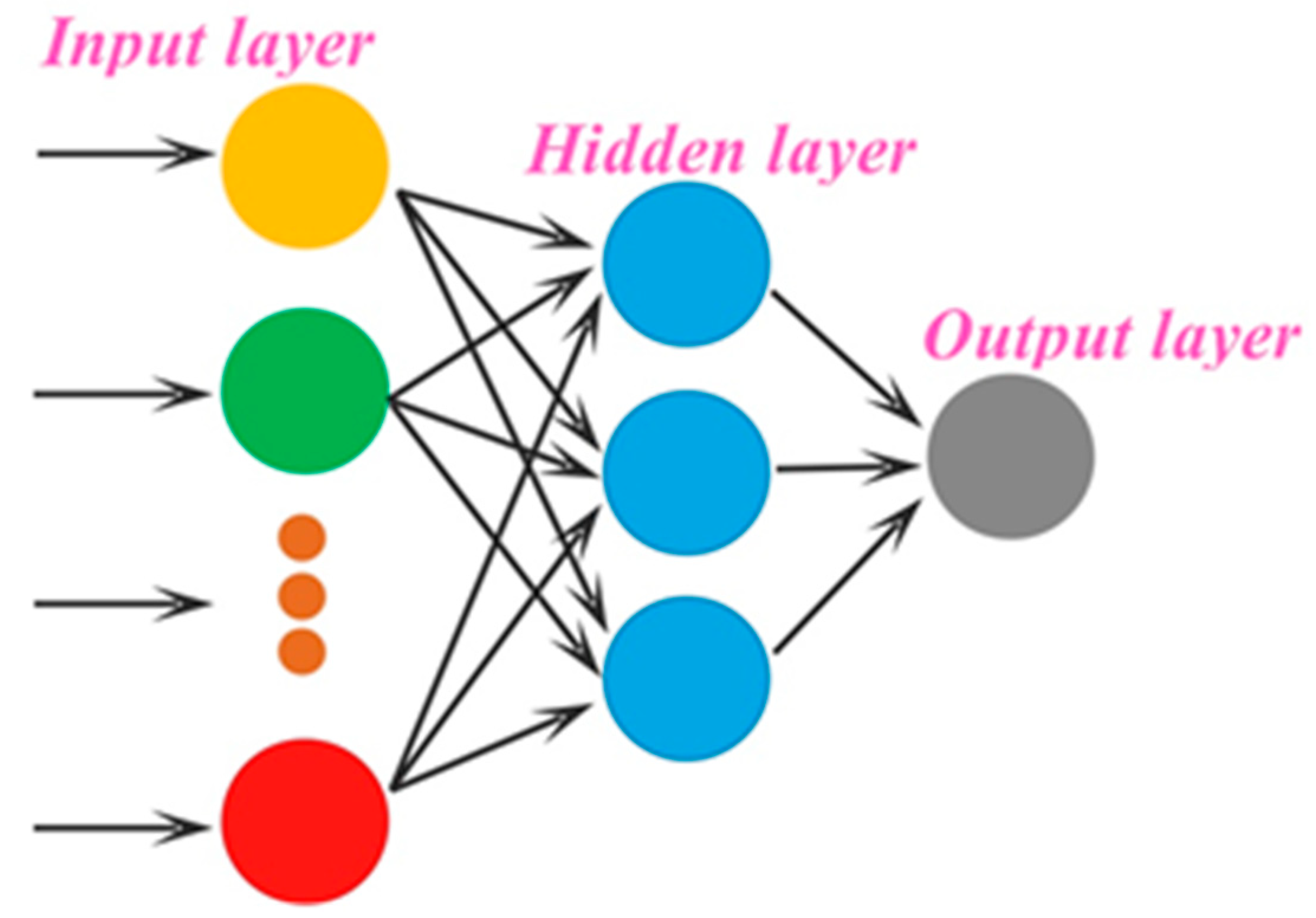
2.1.4. Extreme Learning Machine

Extreme Learning Machine (ELM) is a promising artificial neural network method introduced by Huang which has very fast learning capability [30]. ELM has a simple three-layer structure: an input layer, output layer, and hidden layer, which contains a large number of nonlinear processing nodes [31]. The ELM structure of multiple inputs and a single output is shown by Figure 1. One advantage of ELM over traditional neural networks is that it is not necessary to adjust parameters iteratively. Thus, ELM has a much faster training process with better performance in some cases when compared with traditional neural networks [32]. However, ELM is always applied for balanced data. Imbalanced data problems require special treatment because characteristics of the imbalanced data can decrease the accuracy of the data [33].

2.1.5. Cuckoo Search

The Cuckoo Search (CS) is a new meta-heuristic animal-behavior-imitation algorithm developed by Yang and Deb in 2009 [34]. The CS is always based on three idealized rules: first, each cuckoo can only lay one egg at a time, and lay it in a randomly chosen host bird nest. Second, the best nests with high-quality eggs (solutions) can also be selected by the next generations. Last, the number of available host nests is fixed, and a host bird can discover an alien egg with probability p_a ∈ [0, 1] [35]. Moreover, the performance of the CS can be improved by the usage of Lévy flights. The following Lévy flights are performed:

$$x_{t+1,k}=x_{t,k}+\partial \oplus L\left(\alpha \right)\left(k=1,2,\cdots ,n\right)$$

(13)

$$\partial ={\partial }_0\left(x_{t,k}-x_b\right)$$

(14)

$$L\left(\alpha \right)\sim u={\lambda }^{-\partial }$$

(15)

In these formulas, the step size ($\partial$) is related to the scale of the problem of interests [36], and $\oplus$ expresses entry-wise multiplication locations.

Due to the outliers in the collected data set, the prediction results of the Extreme Learning Machine are not very good. In order to overcome the weakness of the ELM model, one ELM model optimized by Cuckoo Search is developed in the paper. The computational steps of the optimized algorithm (CS-ELM) are described as Algorithm A2.

2.2. Wind Speed Empirical Analysis

Based on the data of Dangjin Mountain in Akeisai, China, the part uses MAE, RMSE and MAPE as prediction evaluation indexes, builds a model after statistical analysis and data preprocessing, and gets results.

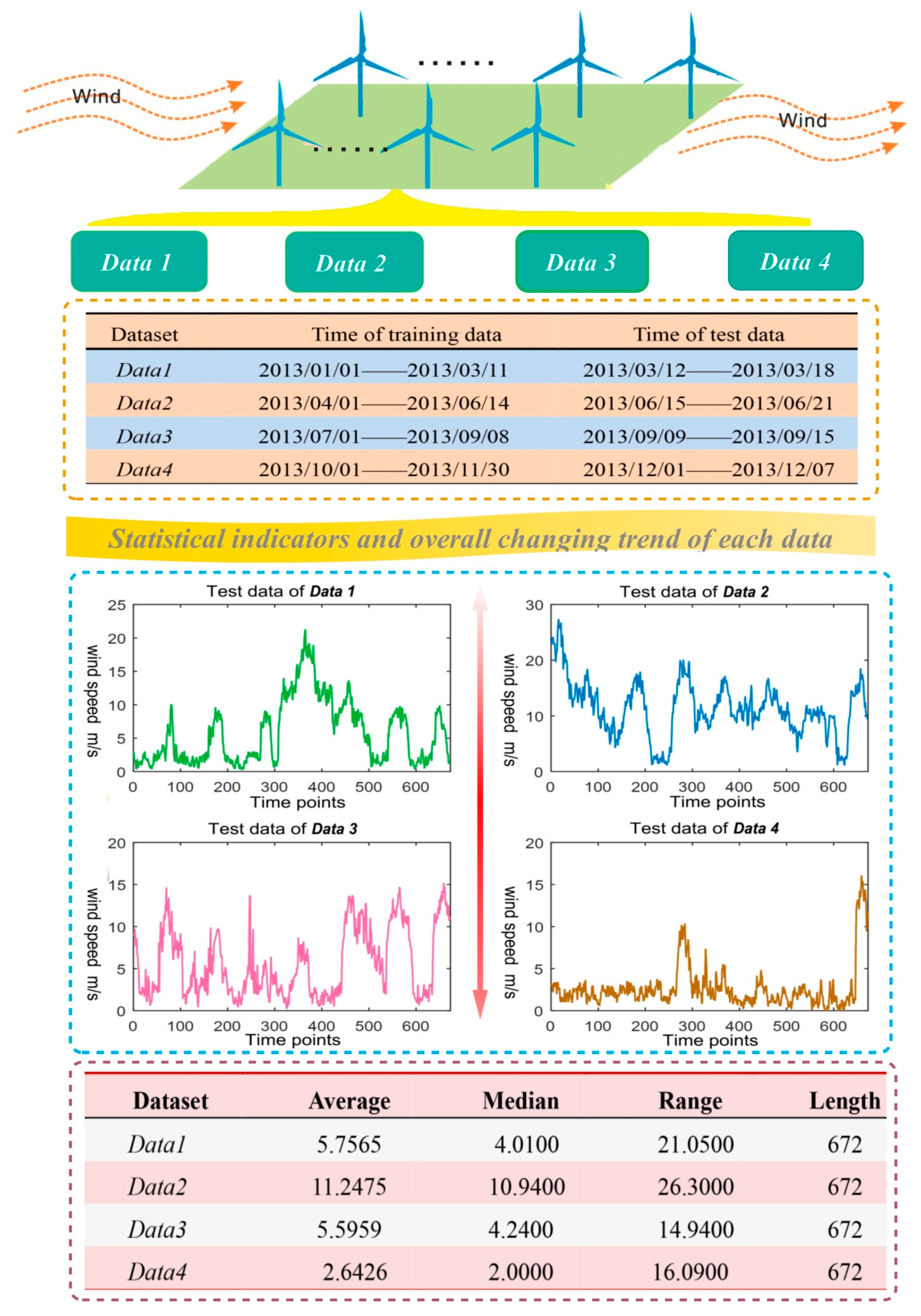
2.2.1. Data Resources

Dangjin Mountain wind farm in Akesai is the first plateau type of demonstration wind farm established in our country and has been in use since 2010. In 2014, the wind farm had an electricity installment capacity of approximately 100 MW and provided surrounding areas with green and clean energy add up to 4.58 billion kWh [37]. The wind speed data collected every 15 min from 1 January to 31 December in 2013 for Akesai Dangjin Mountain wind farm is referenced for empirical analysis data in the experiment.

2.2.2. Prediction Evaluation Index

Let the forecasting target outcome be $y^{\mathrm{target}}\left(n\right)\in {\mathbb{R}}^N$ for $n=1,2,\cdots ,\mathrm{T}$ presenting forecasting temporal points. To evaluate the accuracy of the output result $y\left(n\right)$, mean absolute error (MAE), root mean square error (RMSE) and mean absolute percentage error (MAPE) are applied as prediction evaluation indexes and the equations of these indexes are shown as

Table 1. Three prediction evaluation indexes.

Metric	Definition	Equation
MAE	Mean absolute error	$MAE=\frac{1}{T}{\displaystyle \sum _{n=1}^T\left|y^{\mathrm{target}}(n)-y(n)\right|}$
RMSE	Root mean square error	$RMSE=\sqrt{\frac{1}{T}{\displaystyle \sum _{n=1}^T{(y^{\mathrm{target}}(n)-y(n))}^2}}$
MAPE	The average of the absolute errors	$MAPE=\frac{1}{T}{\displaystyle \sum _{n=1}^T\left|\frac{y^{\mathrm{target}}(n)-y(n)}{y^{\mathrm{target}}(n)}\right|}\times 100\%$, $y^{\mathrm{target}}(n)>0$

.

When these three indexes are smaller, single point prediction is more accurate and the applicability of the proposed model is better.

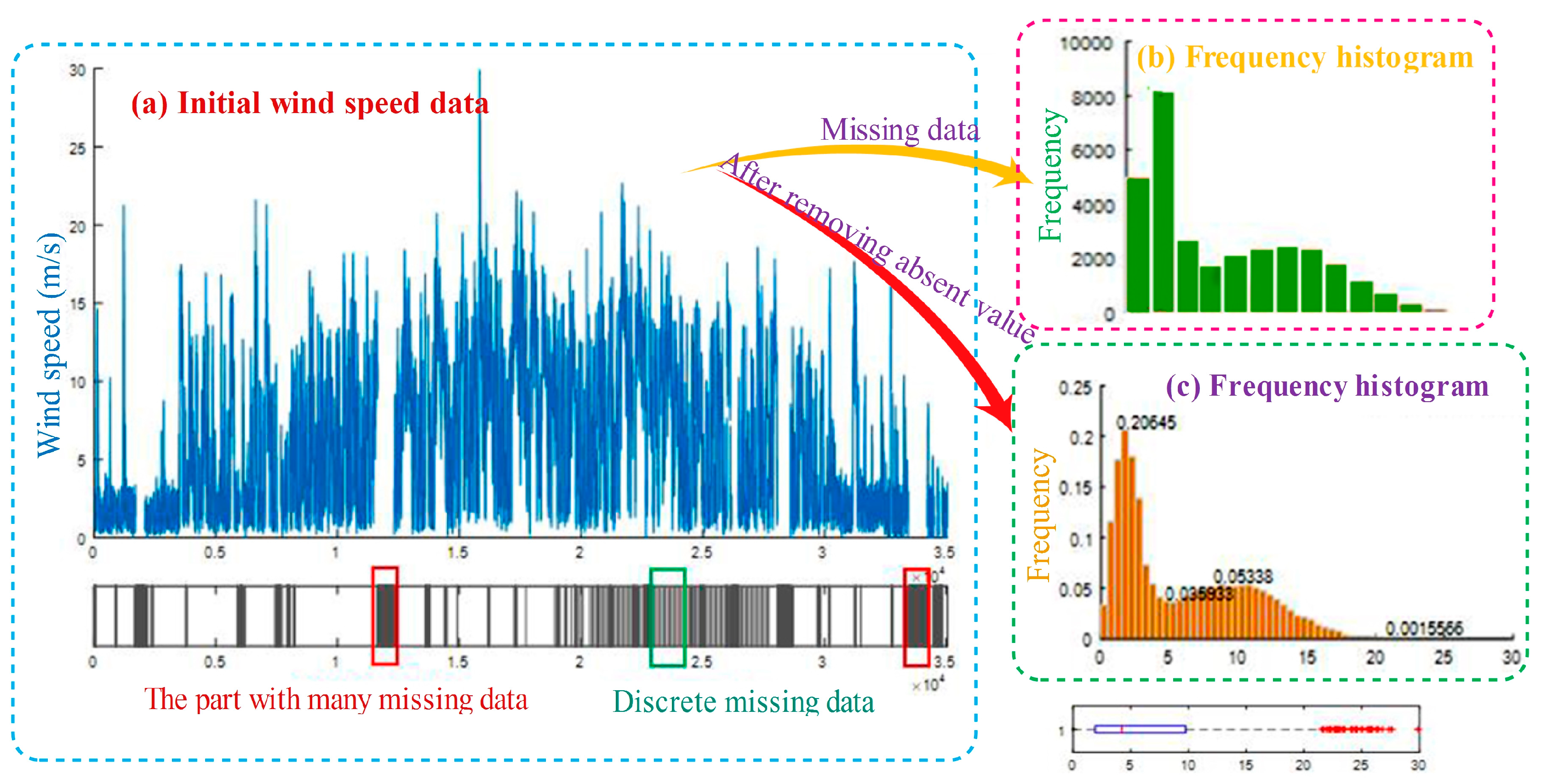
2.2.3. Statistical Analysis and Data Preprocessing

The wind speed data collected every 15 min covering the period from 1 January to 31 December in 2013 for Akesai Dangjin Mountain wind farm is used as empirical analysis data in the experiment. As shown in Figure 2a, the general trend of annual raw wind data demonstrates that the data fluctuation frequency is large and that there are many cuspidal points. The data value on both sides is small, but there is a peak in the middle. In addition, because of the existence of data loss, the diagram also presents the wind speed data collection. The grey line indicates that the data are missing at that position or that the value is the same at different times. It is estimated that the amount of missing data takes up 12.2% of the total samples.

Figure 2b shows the frequency histogram after removing missing data. It’s easy to be seen from the frequency histogram that with the influence of significant missing data, the collected data does not obey the single peak statistical distribution, but has complex statistical characteristics. The boxplot below clearly reflects the range of 0~4 m/s, focuses nearly 50% of the data, and the other distributes in the range of 4~30 m/s more dispersedly. From this, it can be seen that the local has rich wind resources. Therefore, setting up accurate wind speed forecasting model is significant to the effective usage of wind energy for the region.

To estimate the probability density function of collected wind speed data, the probability histogram and the Freedman-Diaconis Rule function are applied to calculate $h$. In statistics, the Freedman-Dacoins rule can be used to selected the size of the bins to be used in a histogram [38]. For a set empirical measurements sampled from some probability distribution, the Freedman-Doaconis rule is designed to minimize the difference between the area under the empirical probability distribution and the area under the theoretical probability distribution. According to the Freedman-Diaconis Rules, $h=2\times IQR\times n^{-1/3}$. The calculation result shows that $h=0.5010$ and that the probability of points falling into the range of 5~30 m is 0.5095. Figure 2c provides the probability histogram after removing missing data.

In the process of collecting data, the situation of collecting unreal data resulting from transmission error, instrument failure or special weather often appears. These data perform as abnormal and missing two cases and would influence further analyzing and forecasting by negative trends. To make the process of analyzing and predicting complete and the results more reasonable, the method of processing outliers and interpolating missing data is employed as follows.

The section takes the wind speed data as random dynamic signal and adopts the absolute mean value method to remove outliers. The underneath of Figure 3 shows existing minimax value segment in the empirical data adding up to 1000 from 20:00 on 15 February 2013 to 5:45 on 26 February 2013. The section applies $\tau =10,k=4$ and $\tau =50,k=5$ two parameter combinations, respectively, to remove the maximum point and minimum point. According to detected outliers by Dynamic Absolute Mean Value method (as shown in Figure 3), red dot and yellow dot present the extreme value point through the first and second parameter combination.

The recognition results of outliers with different segmentation length $\tau$ and coefficient $k$ are presented in Figure 3. From this, it is easy to draw the conclusion that using a single parameter combination is difficult to recognize all maximum and minimum value points comprehensively and is possible to eliminate the abnormal points. In addition, when the coefficient $k$ is the same and the segmentation length $\tau$ is different, both the subscript and the number of recognized points are different. Then, with the same $\tau$ and an increasing $k$, both the rejection range and the number of found extreme value points become smaller. This is the reason why we apply two different parameter combinations to remove outliers. Figure 3 also lists the points’ subscript with different coefficients. Moreover, there are a few single points absent in the original data distribution. Combined with the above eliminated outlier, the Cubic Spline function is selected to interpolate the missing value in the data. Missing too many data cannot achieve satisfied result, so the segments missing more than 20 values are excluded in the section.

Figure 4 shows the wind speed data for empirical research after the removing of outliers and interpolating missing data. Compared with Figure 2a, the effect of the Dynamic Absolute Mean Value method in removing outliers and the practicability of Cubic Spline Interpolation are ensured. From Figure 4, it can be observed that there are only 20 or more values that are empty in processed missing data segments. In the subsequent study, the overall data are decomposed into four datasets for empirical analysis according to the position of these nulls.

Table 2. Several statistical indexes before and after data interpolation.

Index	Before Interpolation	After Interpolation
Median	4.23	4.23
Average	5.99	6.00
Range	29.88	29.88
Skewness	0.74	0.74
Kurtosis	2.57	2.57

lists several statistical indexes, such as median and range before and after data interpolation. As can be observed, in these indexes, the average is slightly larger, and the rest values are the same as the original data, which suggests the preprocessing in the paper retains the basic characteristics and changing trend of the original data. In other words, the preferred method of removing extreme points and interpolating missing data is effective.

2.2.4. Model Building

This section proposes building a wind speed forecasting model where random initial input weights and the threshold in the ELM method are optimized by Cuckoo Search. The framework of the entire optimization model is shown in Figure 5. The specific modeling process is as follows:

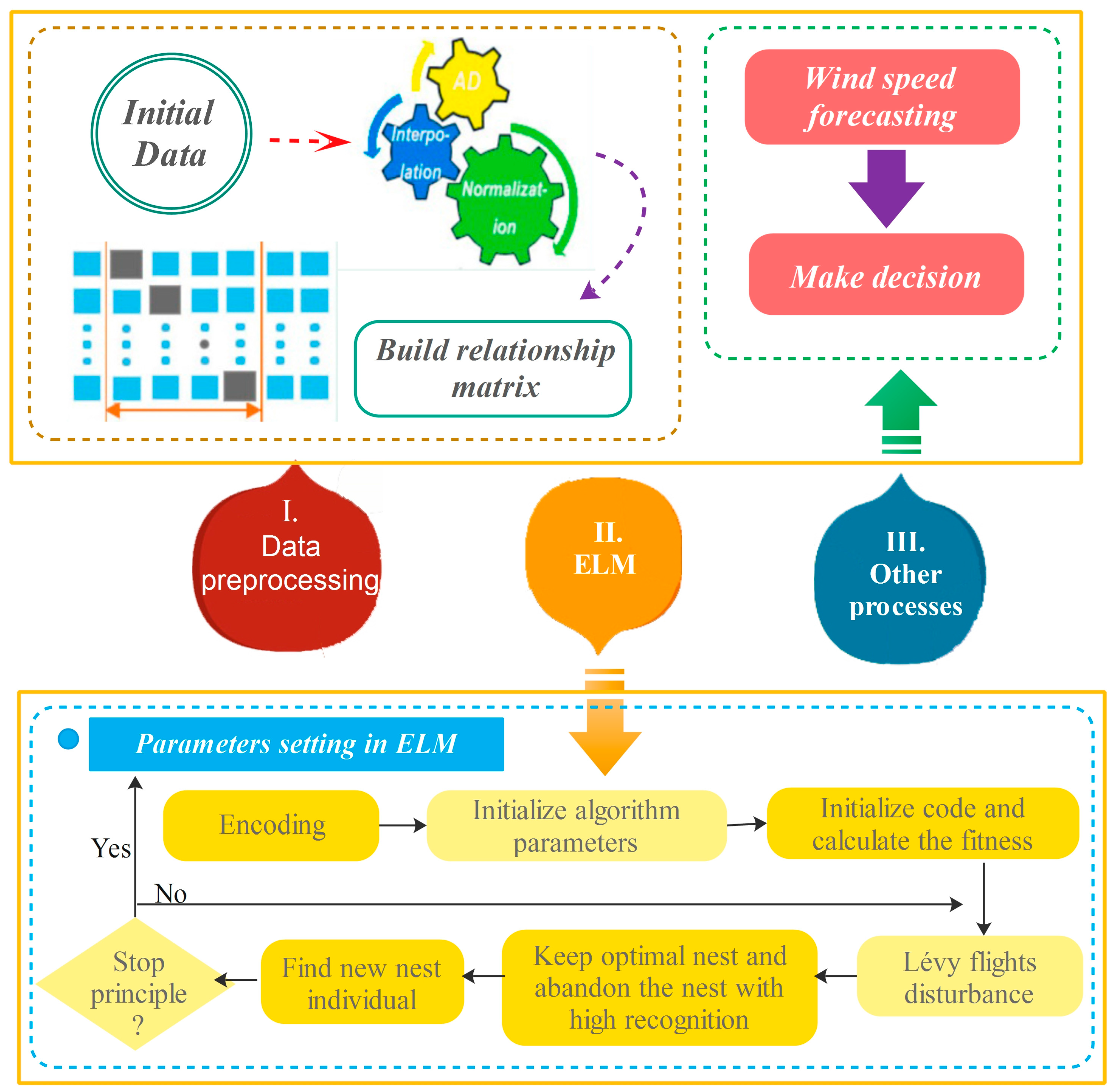
• Step 1. Data processing: The scope of the outlier to be removed can be defined by the Dynamic absolute mean value method, and after eliminating outliers, Cubic spline interpolation is used to complete data. Normalize the input data to eliminate the null column in the transformation data matrix and avoid the influence of data in results obtained by ELM as much as possible.
• Step 2. Parameter setting: Set the number of hidden layers and the activation function in ELM and the number of iterations, nest number, host recognition, boundary conditions and objective function in CS. Due to the weights in the interval [−1, 1] and the threshold in [0, 1], the parameter of the different parts of each individual coding need to be set with different scopes. The situation in which a portion of the individual is beyond the scope in iterating should employ re-initialization. The objective function decides the search trends and the results of the algorithm. The section employs 10-fold cross-validation mean square error sum as the output value of the objective function. Then, screen the optimal weight and threshold on the basis of this. As a result, the possibility of being selected is higher with higher fitness.
• Step 3. Encoding: Code for individuals $w_{11}{w}_{12}\cdots w_{1p}{w}_{21}{w}_{22}\cdots w_{2p}\cdots w_{N1}\cdots w_{Np}b{s}_{1}b{s}_2\cdots b{s}_N$ where $w$ denotes the weight and $bs$ denotes the threshold. In the initial phases, the first $N\ast p$ weights are initialized by the usage of the real random number in [−1, 1], but the rest part is initialized by the number in [0, 1].
• Step 4. Optimization iteration: firstly initialize the fitness of the nest, use the initial optimal nest individual and Lévy flights disturbance to generate new individuals, and calculate the fitness values of all nest individuals after disturbance. Write the fitness of nest $i$ as $O(i)$ and the new nest fitness as $O\left(i^{\prime }\right)$. If $O\left(i^{\prime }\right)<O\left(i\right)$, then replace the nest $i$; in every generation save the nest with small fitness, abandon the host nest with high recognition and find a new nest individual again.
• Step 5. Test: The optimized weights are used as the input weights in ELM to build the optimized wind speed prediction model.
• Step 6. Reconstructed model: Set a single point prediction threshold. If ELM forecasting values are continuously above the prediction threshold, re-optimize and adjust the weights.

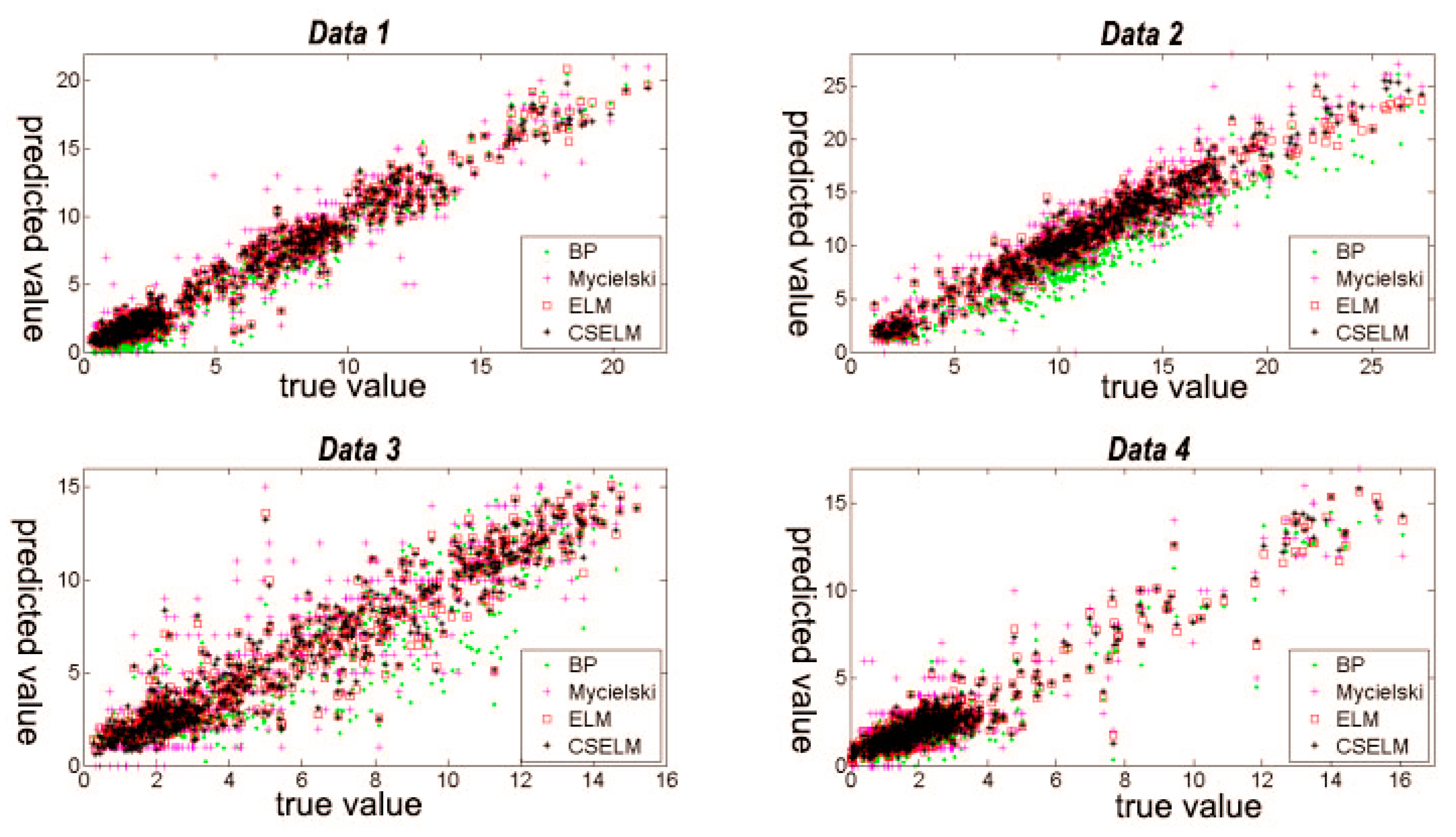
2.2.5. Model Results

In this section, BP neural net, Mycielski and non-optimized ELM are used as contrast models to analyze the predictable performance of the ELM model optimized by the Cuckoo algorithm proposed in the previous section. To ensure the model’s rationality, node number of input and hidden layers of BP, non-optimized ELM and CS-ELM are set to be the same. Moreover, the $Sigmoid$ function is used as the activation function in three models. The parameter of the $\mathrm{CS}\text{-}\mathrm{ELM}$ model is set as follows: let the nest number $n=50$, the host recognition $p=0.25$, the number of iterations $N=100$, node number of input $inputnum=11$ and hidden layers $hidnum=20$. Moreover, $Sigmoid$ function is the activation function, the weight is in [−1, 1], and the threshold is in [0, 1].

To reflect the forecasting effect of each model in different months and seasons, the annual data are divided into four datasets referred to as Data 1, Data 2, Data 3 and Data 4. In the section, at least two months of data are used for training and the weeklong prediction is selected for evaluating the performance of each model. Figure 6 lists the training data and time of the four datasets corresponding to four seasons from top to bottom.

For convenience in contrasting the effects, Figure 6 also shows the basic statistical value of data use in four datasets. The test set length of all four datasets is 672, presenting collected wind speed data in seven days. In Data 2, the average wind speed is 11.2 m/s and the median is 10.94 m/s, illustrating the wind is strong in the period. The wind speed is 2.64 m/s on average in the low wind period, Data 4. The statistical indicators of Data 1 and Data 3 are similar. From range, it can be observed that all four datasets have windy days. The range of Data 2 reaches 26.3 m/s, and Data 1 also reaches 21.05 m/s. It suggests that the size and type of the local wind is various and that the wind energy resource is abundant. In this case, establishing an accurate wind speed forecasting model is particularly important.

Figure 6 presents the line chart of four test datasets at the same time, clearly describing the overall changing trend of wind speed in four seasons. As shown in Figure 6, the data in Data 4 is stable and the overall value is small. Data 2 and Data 3 fluctuate wildly, accompanied by certain periodicity. Both sides of the Data 1 value are small, and the middle value is large.

Figure 7 includes figures that present the contrast between the true value and the predicted results obtained by the different models on the basis of four datasets. There, the horizontal axis is the real value, and the vertical axis shows the prediction result. Clearly, when the points are closer to the diagonal, the prediction effect is better. In Data 1, it is evident that the predictions of ELM and CS-ELM are close and focus around the diagonal, the Mycielski model is more dispersed, and the points of BPNN are in the range of 0–10 m/s and off to the real value, demonstrating that the prediction results are small. In the contrasting processing in Data 2, the points of BP off to the true value and Mycielski off to the prediction show that both models are biased for Data 2. The results of ELM and CS-ELM are close and more concentrated, suggesting that the two models have an advantage in the group. From the third figure, it can be seen that the prediction effect of the four models is unsatisfied, and among them, the Mycielski method is the worst one. For Data 4, the points are mainly in the range 0–4 m/s, and the four algorithms are similar. The forecasting results of the part more than 0–4 m/s are dispersed. Based on the overall situation in four datasets, the following conclusion can be draw: the effect of ELM and CS-ELM is satisfied relatively, while the results of BPNN and Mycielski are often dispersed.

Moreover,

Table 3. The results of the optimized model and contrast model.

Datasets	Model	RMSE	MAPE (%)	MAE
Data 1	BP	1.2937	37.7885	1.0574
	Mycielski	1.3973	32.0933	0.98815
	ELM	0.95513	22.0223	0.70935
	CSELM	0.95154	21.9128	0.70312
Data 2	BP	2.47	20.8619	2.0638
	Mycielski	1.8098	15.9512	1.3655
	ELM	1.2884	11.365	0.97447
	CSELM	1.2069	10.98	0.92169
Data 3	BP	1.7408	32.5512	1.231
	Mycielski	1.7999	38.1428	1.2921
	ELM	1.2618	29.0563	0.88979
	CSELM	1.2582	27.8345	0.88564
Data 4	BP	0.83373	57.8981	0.60687
	Mycielski	1.1868	69.887	0.85244
	ELM	0.80629	49.52	0.57975
	CSELM	0.78449	49.0454	0.55874

collects the prediction evaluation indexes of different models in the four datasets. Overall, the prediction effect of ELM and CS-ELM is much better than that of BP and Mycielski. In Data 1 and Data 2, the performance of BP is worse than Mycielski, while in Data 3 and Data 4, Mycielski is worse. This is because initial weights have a great influence in BP, and different random initialization results led to different prediction results. Next, in view of the above four dataset results, after being optimized by CS, the ELM effect achieves a certain improvement. The improvement is the most obvious and the degree is the highest in Data 2 which can be seen by comparing the values of the RMSE, MAE and MAPE. In regard to other datasets, only the performance of CS-ELM has a weak improvement.

Figure 8 shows the contrasting error boxplot of each model for four datasets, in which 1 represents the BPNN model, 2 is the Mycielski model, 3 shows ELM and 4 represents the CS-ELM model. Then, the following conclusions would be introduced:

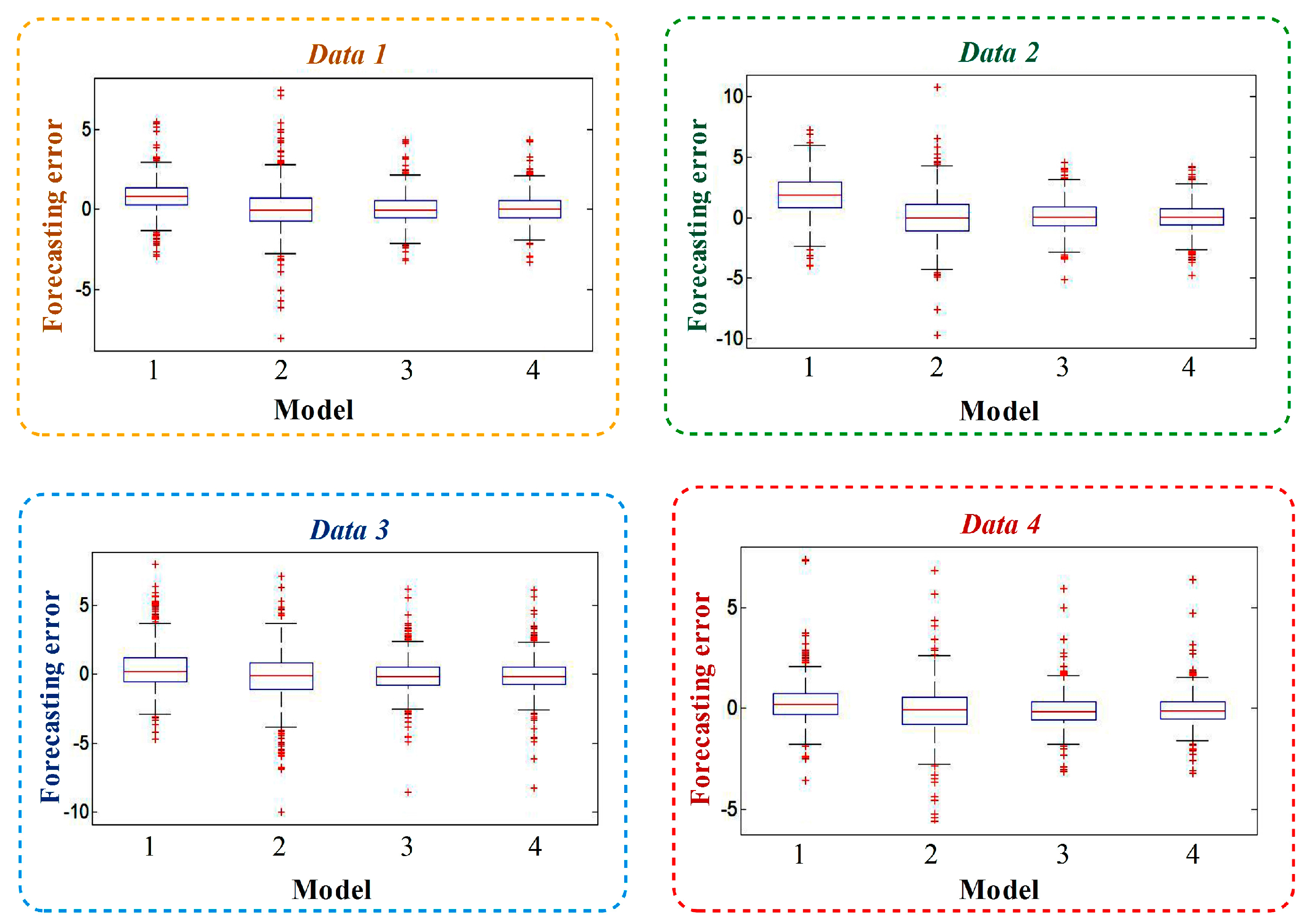
(a)

In the first figure, the prediction result of BP is biased, and the part beyond quartiles is greater. The data of the Mycielski model beyond the upper and lower edge is more and the range of error distribution is wide, presenting an error interval that is maximized. In ELM and the CS-ELM model, the data mainly focuses on the range of −2 m/s~2 m/s, the excess part is less than BP and Mycielski, and the prediction effect is better.

(b)

In the second figure, the error range of the Mycielski model reaches [−10, 10], showing that the performance is very unsatisfied. The overall error is concentrated for ELM and CS-ELM.

(c)

In the last two figures, the result of BP is not obviously biased, and the data range beyond the top and bottom edge is less than Mycielski, so the performance is better than Mycielski. However, its error concentration is not higher than ELM and CS-ELM, leading to worse performance than ELM and CS-ELM.

2.3. Summary

This section applies Cuckoo Search to optimize the weight parameters of ELM. In accordance with the problem that ELM is sensitive to input data, the Dynamic Absolute mean value and Cubic Spline are used to reject outliers and interpolate parts of the missing data, which maintains the integrity of research data well.

In addition, to increase the stability of the proposed model, the rest of the data having more vacancy is removed after setting up an input and output mapping matrix net. Then, optimize the weight parameters of ELM by CS and build the optimized CS-ELM model. Based on the above analysis of the wind speed of Akesai Dangjin Mountain in four seasons, CS-ELM achieves much better accuracy than the other models, and its single-point prediction effect is best followed by ELM. The effect of BP and Mycielski is the worst. Therefore, through optimized weights and a threshold by CS and ELM, the model performance has an improvement, but the improvement is affected by the test set. The wind speed has considerable difference in different seasons, so both the prediction error distribution and results are different for different datasets.

3. Proposed Hybrid Model

Based on CS-ELM prediction model, the chapter mainly studies the following two questions: (1) proper simplified input regardless of the precision of the model; (2) how to provide the range of the forecasted points. To solve the first problem, a hybrid model based on the SGA and ARMA is developed. The SGA plays the main role, which simplifies input in the hybrid model, and ARMA is used to adjust the errors. For the second question, the interval prediction based on the distance cluster is proposed with the application of the filter input.

The remainder of the section is organized as follows: the theoretical part describes the SGA, ARMA and the modeling procedure. The empirical part first presents specific modeling steps, and then the point and interval forecasting results of the hybrid model are given on the basis of the wind speed of Akesai Dangjin Mountain in four seasons.

3.1. Theoretical Analysis

In the chapter, the Standard Genetic Algorithm is used for data filtering to achieve the goal that partial data can obtain higher prediction accuracy. In the end, ARMA model is employed for error correction. Based on the standard genetic algorithm SGA, ARMA time series and CS-ELM model developed in the second section, a hybrid model is proposed in this part.

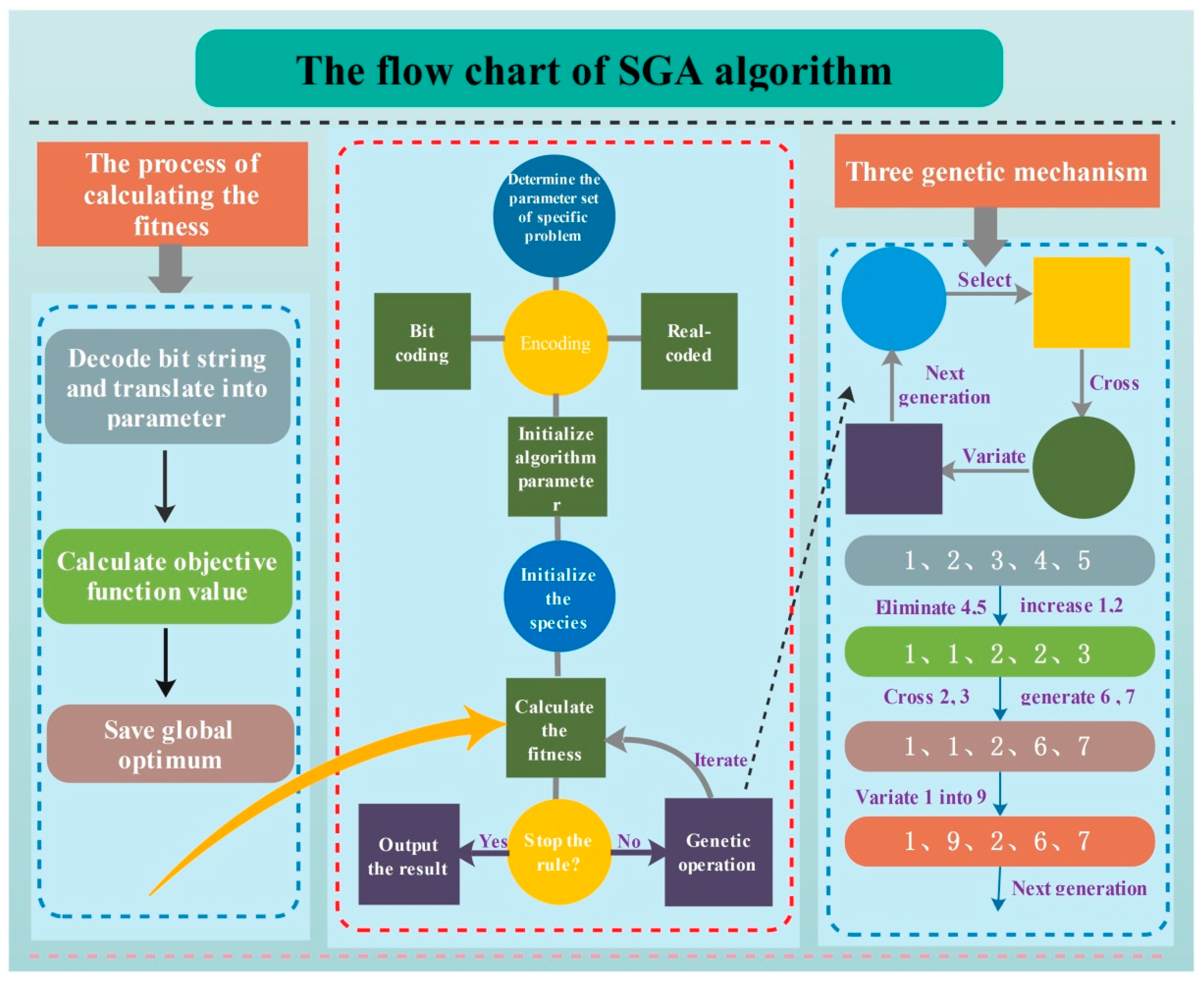
3.1.1. Standard Genetic Algorithm

The Genetic Algorithm (GA) is a powerful stochastic algorithm based on simulating biological genetics and natural selection mechanism’s biological evolution process [39], which was first described in the Ph.D. thesis of Bagay in 1967 [40]. GA starts with an initial set of random solutions called a population, and each individual in the population is called a chromosome [28].

To qualitative analyze the global convergence of SGA based on binary encoding, Holland has established the model theorem and implicit parallelism, proving that SGA can keep the optimal solution in each generation before or after selecting the operation and the result of SGA converge to global optimal solution with probability 1 [41]. Because of its characteristics of uncomplicated operation and parallel searching of the global space, SGA has been successfully utilized in optimal control and machine learning field.

The standard Genetic Algorithm flow chart is shown in Figure 9.

3.1.2. Stationary Time Series

The stationary of one time series includes strictly stationary, wide stationary and non-stationary. In practical application, the stability of one time series can be determined by its statistical properties, such as the mean, variance and so on.

The white noise test: if the time series $\{{\mathrm{X}}_t,t\in T\}$ meets:

$$\left(\mathrm{a}\right)\forall t\in T,\mathrm{E}{\mathrm{X}}_t=\mu$$

(16)

$$\left(\mathrm{b}\right)\forall t,s\in T,r\left(t,s\right)=\{\begin{array}{l}{\sigma }^2,t=s\\ 0,t\ne s\end{array}$$

(17)

then $\left\{{\mathrm{X}}_t\right\}$ is a white noise sequence.

Only when the single variable time series meets stationarity and passes the white noise test, a stationary time series model can be build. The commonly used regression models are the AR model, MA model and ARMA model.

After building the regression model, it’s necessary to verify the fitting effect of the selected model, which is to test the stability of the error.

There are two types of error stationary tests—figure tests and statistic tests—for error sequences. A figure test is a test method utilizing a drawing sequence diagram and autocorrelation. There, the commonly used test methods are the ADF test, PP test and so on. The Daniel test comes to the conclusion through the Spearman rank correlation coefficient $q_s$ passing the hypothesis test:

$$q_s=1-6{\displaystyle \sum _{t=1}^n\frac{{(t-R_s)}^2}{n(n^2-1)}}$$

(18)

3.1.3. Problem Description and Solution

In the previous section, the established model can be expressed as:

$$y_i=f(x_{1,i}+x_{2,i}+\cdots +x_{p,i})+{\epsilon }_i$$

(19)

where $x_{1,i},x_{2,i},\cdots ,x_{p,i}$ expresses the input variables of the model, $p$ represents the dimension, $i$ shows the $i$th column of the input matrix, $f(·)$ represents the built CS-ELM model, $y_i$ is the target output, and ${\epsilon }_i$ shows the error. Moreover, when applying a neural network to build the model, it is generally suggested that variables without high correlation are applied as input. However, in the previous section, the transformed original data matrix is used directly for output-input mapping where the data are in time order and the input has high correlation. Thus, SGA is developed to filter the transformed matrixes. The screening input is used as the input of CS-ELM. Then, adjust the errors with ARMA, achieving the establishment of the hybrid forecasting model. The process of SGA variable selection method joint in the model is shown as follows:

Assume that the established input-output mapping is such that:

$$y_i=f(z_1{x}_{i,1}+z_2{x}_{i,2}+\cdots +z_p{x}_{i,p})+{\epsilon }_i$$

(20)

where $z_1,z_2,\cdots ,z_p$ represents the coefficient of controlling input for 0 or 1. Thus, $z_1,z_2,\cdots ,z_p$ can be encoded with the binary method, for example, $\mathrm{E}[\mathrm{Y}|x,z=(1,0,1,0)]=x_1+x_3$ and $\mathrm{E}[\mathrm{Y}|x,z=(1,1,0,0)]=x_1+x_2$. Then, choose the corresponding row data as the input of CS-ELM to build the prediction model.

The method of multi-step ahead forecast is that updating the input data by discarding the old data for each loop to perform the prediction. The multi-step ahead forecast is defined as: define the time index $h$ as the forecast origin and the positive integer l as the forecast horizon. Suppose we are at time index $h$ and intended to forecast ${\hat{r}}_{h+1}$, where $l\ge 1$. Let ${\hat{r}}_h(l)$ be the forecast of $r_{h+1}$, then we defined ${\hat{r}}_h(l)$ as the l-step ahead forecast of $r_t$ at the forecast origin $h$. When $l=1$, we defined ${\hat{r}}_h(1)$ as one-step ahead forecast of $r_t$ at the forecast origin $h$ [42,43].

The following is the method for building the interval model:

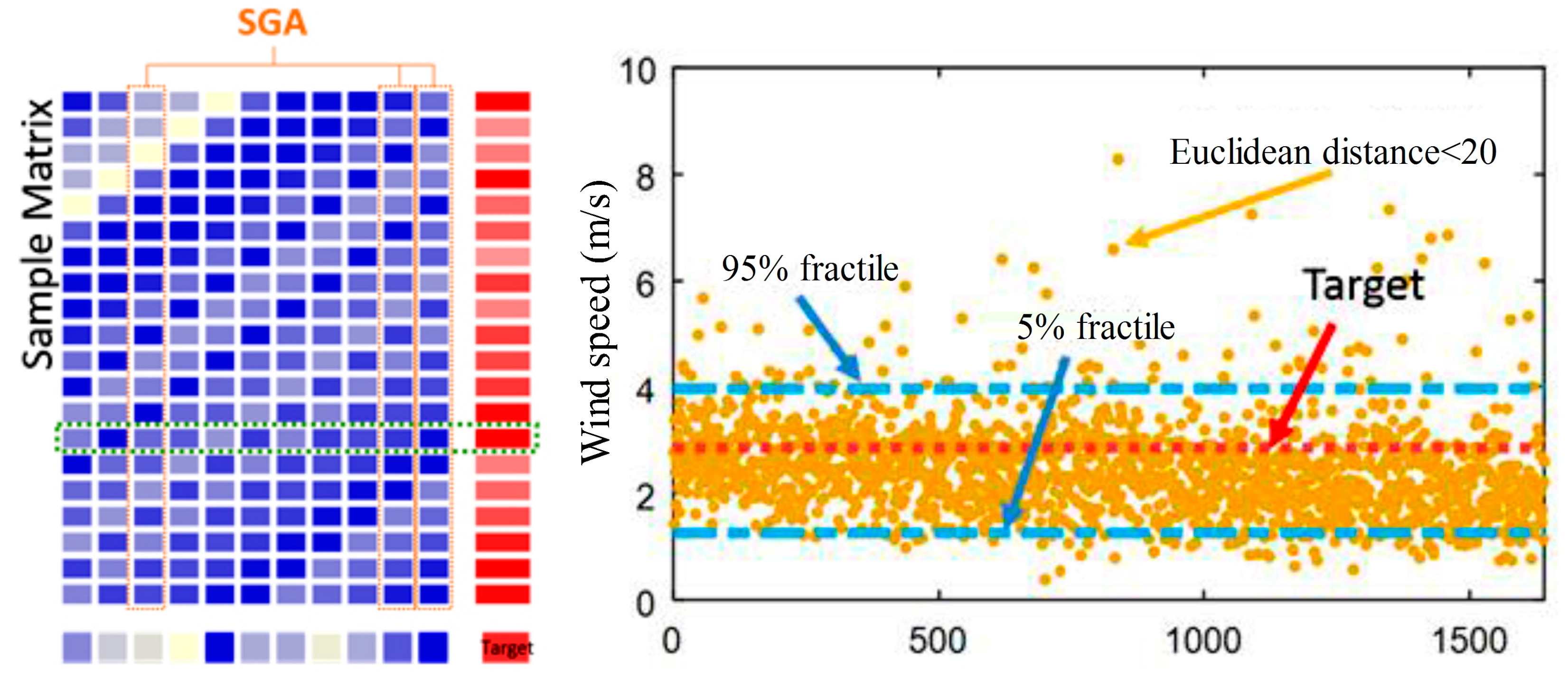
• Calculate the Euclidean distance between the test input vector and training input matrix after screening and arrange according to the values from small to large. Set a distance threshold. Lump the values less than the threshold into one class and find corresponding input vectors to form a new mapping matrix. Because each vector in the new matrix has a small distance with the test input vector, vectors therein are considered as the test input vector joined the interference. At a result, corresponding test output value which is used as a possible sample space of current prediction can be obtained. We select 5% fractile and 95% fractile of the sample as the upper and lower bounds of the confidence interval. However, due to the limited historical data, it is difficult to find close vectors and construct the sample space for the test input vector. For this reason, we can consider the spacing of part points and ignore the distance of other points, which reduces the overall distance and constructs the sample space of similar sequences. Although the SGA-CSELM model proposed in this chapter removes part variables during the input process, its result is similar to that of the CS-ELM model or even better. Thus, the SGA-CSELM screening results are adopted as a new test vector to find the possible forecast sample space again and obtain a confidence interval closer to the forecasting point. Figure 10 is an instance of the prediction point. In addition, for rare points that cannot form intervals, the moving average method is applied to obtain upper and lower boundaries.

3.2. Experiment

The hybrid model proposed in this section takes SGA into consideration, reduces the input variable appropriately and achieves a more powerful forecasting result than the CS-ELM model.

3.2.1. SGA-CSELM Model

The following briefly introduces the process of the construction of the SGA-CSELM combination model:

• Data processing: Build the initial input and output matrix of the CSELM model and then eliminate the null columns in the matrix to ensure the continuity of the data. Normalize the data to reduce the interference of data resources on the ELM.
• SGA parameters setting: Set the appropriate fitness function $F(•)$, write the number of inputs requiring filtering as $n$ and compile the SGA individuals as:

  $$G_k=\left(g_1,g_2,\cdots ,g_i,\cdots ,g_n\right),g_i=0or{g}_i=1$$

  (21)
  Set up the SGA parameters, such as the total number of individuals $N$, number of iterations $Niter$, crossover probability $p_1$, mutation probability $p_3$ and so on.
• ELM parameters setting: Decode the output results of the ELM, extract the corresponding line of the output and input matrix as the model input, obtain the neuron number of the input layer and hidden layer and employ Sigmoid as the activation function.
• CS parameters setting: Set the number of iterations, nest number, host recognition, boundary conditions and objective function. The weight is in the interval [−1, 1], and scope of threshold is [0, 1], so the parameters represented by the different parts of each individual should be set in different ranges. Moreover, generate the portion of the individual out of range by way of re-initialization. The objective function determines the search trends and results of the algorithm, so the paper employs the mean square error of the test data fitting the value $1/mse(\mathrm{y}-\widehat{\mathrm{y}})$ as the output value of the objective function and filters the optimal weight and threshold accordingly.
• Encoding: Apply the coding $w_{11}{w}_{12}\cdots w_{1p}{w}_{21}{w}_{22}\cdots w_{2p}\cdots w_{N1}\cdots w_{Np}b{s}_{1}b{s}_2\cdots b{s}_N$, where $w$ represents the weight and $bs$ stands for the threshold value, for individuals. In the initial phase, the first $N\ast p$ weights are initialized by the usage of the real random number in [−1, 1], but the rest is initialized by the number in [0, 1].
• Optimization iteration: First, initialize the fitness of the nest, use the initial optimal nest individual and Lévy flights disturbance to generate new individuals and calculate the fitness value of all nest individuals after disturbance. Write the fitness of nest $i$ as $O(i)$ and the new nest fitness as $O\left(i^{\prime }\right)$. If $O\left(i^{\prime }\right)<O\left(i\right)$, then replace nest $i$; in every generation, save the nest with small fitness, abandon the host nest with high recognition and find a new nest individual again.
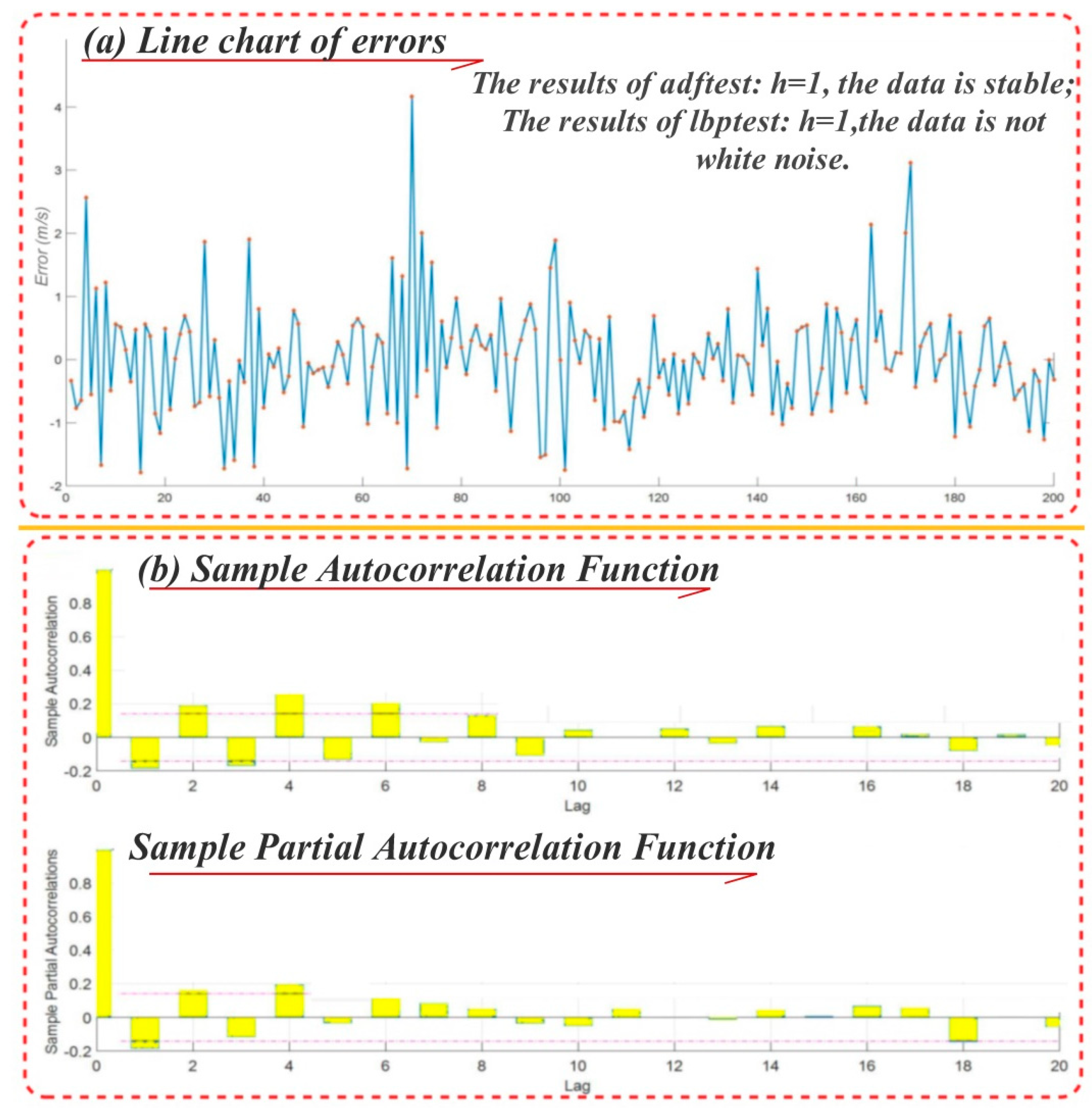
• Carry out test data fitting and obtain the training error: Set the sliding window width H, obtain the training error of the data within the widow width H used to test data and judge whether the data are white noise. If it is white noise, skip the ARMA model building steps, or establish ARMA and carry out step (8).
• Identify the ARMA model: Employ the window width data to calculate the corresponding model lag intervals for endogenous to minimum BIC rule and build the ARMA model.
• Training model: Take the obtained optimizing weights as the input weights of ELM and build the SGA-CSELM hybrid wind speed forecasting model.
• Error correction: Enter the new data into the SGA-CSELM model to obtain the prediction. If there is an ARMA model, then enter the error obtain the error prediction, and correct the error in the SGA-CSELM results to obtain the Hybrid Model.
• Reconstruct model: Set the forecasting threshold of a single point. If the efficiency of the ELM exceeds the threshold continuously, then retrain the Hybrid Model.

3.2.2. Model Results

Apply the GAOT toolbox to build SGA, and the specific parameters are set as follows: the number of iterations is 100, the species number is 20, the crossover probability is 0.09, and the mutation probability is 0.05. It is important to note that, due to variable screening, the input node of CSELM, $inputnum$, varies with the change of screening data. Therefore, when building the SGA-CSELM model, we set the number of hidden layer nodes at the Apply GAOT toolbox to build SGA, and the specific parameters are set as follows: the number of iterations is 100, the species number is 20, the crossover probability is 0.09, and the mutation probability is 0.05. It is important to note that due to variable screening, the input node of CSELM, $inputnum$, changes with the change of screening data. Therefore, when building SGA-CSELM model, we set the number of hidden layer nodes at:

$$hiddennum=2\times (inputnum-1)$$

(22)

To facilitate the efficiency of models quickly, we directly introduce the prediction of ELM and CS-ELM and write them as ELM-1 and CSELM-1. In addition, the ELM model of which the number of hidden layer nodes is the same as screening $hiddennum$ is added, and its efficiency and CS-ELM’s are comprehensively compared. The input of the newly added model and the original one is the same; for the purpose of distinguishing them, they are written as ELM-2 and CSELM-2. Finally, through the test in stationary and white noise for the prediction error of the SGA-CSELM model, the ARMA model is built for the non-white noise part to correct the prediction error. The other parameters of the SGA-CSELM model are set as in the previous chapter.

Selection Results of the Input Variable

Table 4. The screening results of input data.

Dataset	Z	Model	$\mathit{f}\mathbf{(}\mathbf{•}\mathbf{)}$
Data 1	(1,0,0,0,0,0,0,0,1,1,1)	$f(z_1{x}_{i,1}+z_9{x}_{i,9}+z_{10}{x}_{i,10}+z_{11}{x}_{i,11})$	2.6925 × 10−4
Data 2	(0,1,1,0,0,0,0,0,0,1,1)	$f(z_2{x}_{i,2}+z_3{x}_{i,3}+z_{10}{x}_{i,10}+z_{11}{x}_{i,11})$	1.4634 × 10−4
Data 3	(0,0,0,0,0,0,1,1,1,1,1)	$f(z_7{x}_{i,7}+z_8{x}_{i,8}+z_9{x}_{i,9}+z_{10}{x}_{i,10}+z_{11}{x}_{i,11})$	1.2828 × 10−4
Data 4	(0,0,1,0,0,0,0,0,0,1,1)	$f(z_3{x}_{i,3}+z_{10}{x}_{i,10}+z_{11}{x}_{i,11})$	2.7143 × 10−4

lists the output of four datasets after being screened by SGA. The first column presents the four datasets, and the second is the screening binary results, where 0 shows it cannot be chosen as model input and 1 means that it can be chosen. Here, the established input and output matrix is the same as the previous one. The third one shows the input subscript after screening, from which it is easy to see that, for the different stages of data, different input data models should be applied. Among them, the data Data 3 need is the most and Data 4 is the least. The last column describes the fitness function value corresponding to the screening model.

Through this table, the number of input variables and the subscript can also be obtained. For example, in Data 1, the input nodes number is $inputnum=4$, so the corresponding layer nodes in SGA-CAELM is $hiddennum=2\times (inputnum-1)=6$, and the index in contrast model in ELM-2 and CSELM-2 is also 6.

Model Contrast Result

Table 5. The comparison between the predictive indexes of various models in Data 1.

Model	RMSE	MAPE (%)	MAE
ELM-1	0.95513	22.0223	0.70935
CSELM-1	0.95154	21.9128	0.70312
ELM-2	1.0758	26.2801	0.80785
CSELM-2	0.94509	22.1702	0.70205
SGA-CSELM	0.94368	22.0715	0.70112
Hybrid model	0.93729	22.4062	0.69569

shows the prediction results of various models in Data 1. The first column is the six models used in the test. Among them, the results of ELM-1 and CSELM-1 come from the second section, ELM-2 and CSELM-2 are contrast models of which the layer nodes are set as SGA-CSELM, SGA-CSELM is the model that does not join ARMA for error correction, and the last hybrid model is the one joining ARMA. Moreover, the second to fourth columns describe the performance of each model under different indicators. According to the value of the RMSE, the hybrid model’s value is the smallest and the ELM-2′s is the largest. From MAPE, all models are near 22%, the ELM-2 is the biggest, CSELM-1 is the smallest one, and the rest center. The efficiency of the hybrid model is the best, and SGA-CSELM follows from MAE. Taken together, although there is a decrease in the input information of SGA-CSELM after screening the variable, the prediction result is still better than ELM and near CS-ELM. The result of the hybrid model has ascends after error correction by ARMA.

In the process of forecasting, we employ the ARMA time series model and a dynamic test and predict the stationarity of the error and judge whether the error is a white noise sequence. If the conditions of the time series model are met, then build ARMA to fetch useful information for further data. Figure 11a shows the line chart drawn according to 200 points used to construct the ARMA model in Data 1. From the figure, it can be seen that the error fluctuation is larger, and the SGA-CSELM model does not fully extract the data information in the process of training. Apply the ADF test for the sequence; the result indicates that it is smooth. Through the Ljung-Box Q-test, detect the error correlation, not the white noise sequence. Therefore, the ARMA model can be constructed for the data fitting error and further extract the useful information from the error term. Figure 11b is the autocorrelation and partial autocorrelation figure of the segment data, showing that the data fits ARMA (4,6), but in factual modeling, ARMA (1,1) is chosen because, when the orders of both AR and MA are 1, the value of the corresponding criterion is minimum (shown in Table 7) through comparing the criterion value of AIC and BIC, etc.

Table 6. AIC and BIC values in ARMA model with different R, M in the data segment with H = 200.

R	M	AIC	BIC
0	0	525.9757	532.5723
0	1	522.9694	532.8644
0	2	520.4012	533.5945
0	3	520.9191	537.4107
1	0	521.2324	531.1274
1	1	510.6493	523.8426
1	2	511.7579	528.2495
1	3	513.2704	533.0603
2	0	517.0375	530.2307
2	1	511.8597	528.3513
2	2	513.2522	533.0421
2	3	514.3671	537.4553
3	0	516.4494	532.941
3	1	513.6157	533.4056
3	2	515.1741	538.2623
3	3	515.9503	542.3369

lists the AIC value and BIC value for fitting the ARMA model in the data segment with the sliding window width H = 200 when $R=0,1,2,3$ and $M=0,1,2,3$. By comparing the BIC rule in the scope in which $R=0,1,2,\cdots ,6$ and $M=0,1,2,\cdots ,6$, it can be found that, when $R=1,M=1$, the AIC and BIC values are the smallest. Thus, ARMA (1,1) is used to build the model, and in the next H = 200 steps, the error for the SGA-CSELM model is corrected with it.

Table 7. The wind speed forecasting results from 0:15 to 7:00 with each model with part data in Data 1.

Time	Original Data	ELM-1	CSELM-1	ELM-2	CSELM-2	SGA-CSELM	Hybrid Model	Adjusted Value
0:15:00	1.82	2.87	2.7	2.19	2.77	2.86	2.69	−0.17
0:30:00	1.55	1.81	1.72	2.49	1.95	1.78	2.05	0.28
0:45:00	1.53	1.6	1.63	1.96	1.64	1.68	1.49	−0.19
1:00:00	1.14	1.54	1.51	1.5	1.52	1.59	1.74	0.14
1:15:00	0.41	1.11	1.23	1.35	1.34	1.22	1.16	−0.06
1:30:00	0.45	0.55	0.62	1.24	0.66	0.62	0.76	0.14
1:45:00	1.86	0.76	0.66	1.2	0.64	0.71	0.6	−0.11
2:00:00	0.71	2	1.99	1.41	1.85	1.93	1.82	−0.11
2:15:00	0.63	0.77	0.93	1.25	0.95	0.71	0.95	0.24
2:30:00	0.98	0.88	0.94	1.16	0.77	0.9	0.71	−0.2
2:45:00	1.13	1.17	0.96	1.13	1.03	1.15	1.25	0.1
3:00:00	1.33	1.15	1.25	1.03	1.31	1.21	1.1	−0.11
3:15:00	1.54	1.42	1.43	1.43	1.39	1.39	1.42	0.03
3:30:00	1.53	1.78	1.5	2.13	1.55	1.57	1.5	−0.07
3:45:00	1.57	1.57	1.61	1.97	1.64	1.55	1.58	0.03
4:00:00	0.92	1.61	1.69	1.48	1.58	1.59	1.53	−0.06
4:15:00	1.18	0.97	1.05	1.39	1	0.99	1.1	0.11
4:30:00	1.5	1.31	1.24	1.58	1.36	1.33	1.19	−0.14
4:45:00	1.86	1.59	1.54	1.64	1.53	1.52	1.57	0.05
5:00:00	2.61	1.92	1.95	1.97	1.9	1.84	1.72	−0.12
5:15:00	2.63	2.65	2.64	2.44	2.52	2.54	2.5	−0.05
5:30:00	2.02	2.6	2.59	2.61	2.55	2.51	2.52	0
5:45:00	3.01	1.92	2.04	2.18	2.01	1.98	2.03	0.05
6:00:00	2.15	2.98	2.92	2.28	2.8	3	2.8	−0.2
6:15:00	1.86	2.01	1.96	2.4	2.17	2.03	2.28	0.26
6:30:00	2.02	1.86	1.94	2.3	2.01	1.92	1.73	−0.19
6:45:00	1.65	2.1	2.01	2.2	1.94	2.02	2.13	0.1
7:00:00	1.7	1.66	1.7	1.96	1.76	1.65	1.6	−0.05

shows the concrete results of the 1st to 28th points in Data 1 with each model. In the table, the second column is the measurement data, and the following columns are the point prediction results of ELM-1, CSELM-1, ELM-2, CSELM-2, SGA-CSELM and the model joining error correction. The last one is the error correction of the SGA-CSELM model with ARMA (1,1). For facility, all data reserve two decimal fractions. As a result of Table 7, the prediction effect of the Hybrid Model proposed is best, followed by that of the SGA-CSELM Model.

Figure 12 shows the prediction of the hybrid model and the upper and lower bounds of the prediction interval that is composed by 5% fractile and 95% fractile in Data 1, Data 2, Data 3 and Data 4. First, our model prediction is very close to the real sequence, showing that the forecasting effect of SGA-CSELM has a certain improvement after adding the ARMA model to correct the error. Next, our forecasting range includes almost all real values, and the interval width at some points is narrow. However, there is an obvious shortage in that, when the original data increases quickly, the prediction interval cannot well contain the real value, and the effect is better in the decrease part. To see the details of the forecasting results of the Hybrid model, the point prediction performance of Data 1, Data 2, Data 3 and Data 4 is also given in Figure 12 for reference.

Table 8. The RMSE, MAPE and MAE values of many models in Data 2, Data 3 and Data 4.

Dataset	Model	RMSE	MAPE (%)	MAE
Data 2	ELM-1	1.2884	11.365	0.97447
	CSELM-1	1.2069	10.98	0.92169
	ELM-2	1.4416	13.1777	1.1133
	CSELM-2	1.1987	11.0051	0.91502
	SGA-CSELM	1.2077	10.9918	0.91705
Data 3	ELM-1	1.2618	29.0563	0.88979
	CSELM-1	1.2582	27.8345	0.88564
	ELM-2	1.4675	35.7339	1.0631
	CSELM-2	1.2654	28.7894	0.8927
	SGA-CSELM	1.2652	26.9906	0.88335
	Hybrid model	1.2763	26.5807	0.89842
Data 4	ELM-1	0.80629	49.52 *	0.57975
	CSELM-1	0.78449	49.0454 *	0.55874
	ELM-2	0.88965	58.7557 *	0.64605
	CSELM-2	0.79179	47.9399 *	0.56206
	SGA-CSELM	0.78186	49.0009 *	0.55542
	Hybrid model	0.78695	51.3721 *	0.55959

Note: there are zero points in the measured dataset, “*” is the value of MAPE calculated after removing the point.

lists the evaluation index situation of Data 2 after screening, on the basis of predictive results. Different from Data 1, overall, CSELM-2 works best followed by CSELM-1 and SGA-CSELM effects worse than the two models with the small gap. ELM-1 and ELM-2 work the worst. Because the error sequence is white noise after using SGA-CSELM to forecast the test data in Data 2, the prediction evaluation indexes of the Hybrid Model are not shown in Table 8.

According to Table 8 and the value of the RMSE, CSELM-1 works best, followed by SGA-CSELM, and the Hybrid model result is worse than that of CSELM-2 in Data 3. From the point of view of MAPE, the result of the Hybrid model is the best, and SGA-CSELM follows. From MAE, the parameter value of SGA-CSELM is the minimum. Taken together, each indicator in SGA-CSELM performs most stably, but its result is a bit weaker after joining correction by the time sequence, explaining that the ARMA model is not entirely appropriate for the dataset.

Table 8 also presents the prediction index comparison result of each model in Data 4. From the table, we can see that SGA-CSELM is the smallest in RMSE and MAE. CSELM-2 is minimum in the index MAPE, and the MAPE value of the rest of the model is larger, even more than 50%. This is because the wind speed data in Data 2 is generally small and fluctuates frequently, and any small forecast deviation will lead to a sharp fall in results. In addition, the Hybrid Model of the effect is not the best one; this may be due to the error correction for SGA-CSELM, and the selected MA model is not good for modeling of different variance components.

3.3. Summary

Based on the standard genetic algorithm SGA, ARMA time series and CS-ELM model developed in the second section, a Hybrid model is proposed in this section. When building the CS-ELM model in the previous section, all input and output mapping was put in models to test. However, taking SGA into consideration, the section reduces the input variable appropriately and achieves a more powerful forecasting result than the CS-ELM model.

In the process of hybrid modeling, first, make up the input subscript for 0–1 by the binary code and, through the standard genetic algorithm, select a variable to set up the SGA-CSELM model. Second, conduct the stationarity and white noise test for the prediction error of the SGA-CSELM model. If the error series meets the ARMA modeling conditions, then identify the optimal model by the AIC and BIC information rules. Thus, establish the SGA-CSELM model with error correction, namely, the Hybrid Model. Through empirical analysis of the four datasets of Dangjin Mountain in Akesai, the following results are produced:

• Under the influence of different initial weights, the effect of the single extreme learning machine model changes greatly; nevertheless, the ELM model optimized by the cuckoo algorithm possesses both a stable result and a reliable output guarantee.
• Selecting input variables by the usage of SGA reduces the information of the part variables to some extent, but its prediction effect can still achieve results that are not weaker than those of CS-ELM, which all inputs test.
• The error of SGA-CSELM is corrected by the ARMA model, and the performance of the hybrid model after calibration is improved and declines because during the process of fixing the width of the sliding window, the error may become a white noise sequence and join the error correction, leading to poor results.
• With the screening result of SGA, by calculating the distance between the predicted sample and constructed historical data-mapping matrix, possible forecast points of the sample can be screed to be composed of points that are close. The upper and lower bounds of the prediction sample constructed by calculating the 5% and 95% fractile numerical values obtain a good result.

4. Conclusions

Because existing fossil fuels cannot meet the increasing energy demand, increased attention has been paid to wind energy, a type of clean and renewable energy. However, owing to the intermittency and random character of wind speed, it is essential to build a wind speed forecasting model with high-precision for wind power utilization [44]. Therefore, this paper contributes to the development of an improved wind speed forecasting method [45].

In the paper, the optimized CS-ELM model is applied as the main model, joining SGA and ARMA to build a hybrid model. Based on a series of empirical analyses, the performance of the optimized CS-ELM model is found to overcome the limitations of the single ELM model, that is, it is easily affected by the initial weights, fluctuates, cannot provide stable prediction results and so on. Compared with BP and the single extreme learning machine model, the model has achieved a great improvement in the prediction effect and stable prediction results. It is easy to see that after SGA screening, the model only requires data of lower dimension to produce better prediction results than the single ELM. The ARMA model is employed for error correction to further extract useful information in error prediction. In addition, based on the SGA screening results, by calculating the distance between the test input vector and mapping matrix, building a possible prediction sample space and providing the rough range of the upper and lower boundaries of the predicted values has yielded an excellent performance. Providing an increased accuracy forecasting range can prevent the dramatic fault of a single point prediction, which on a windy day, allows managers to take measures in advance to protect the fan from damage and to have a more competitive advantage to drive markets.

References

- Zahedi, A. Australian renewable energy progress. Renew. Sustain. Energy 2010, 14, 2208–2213. [Google Scholar] [CrossRef]
- United Nations (UN). Sustainable Energy for All; United Nations: New York, NY, USA, 2012. [Google Scholar]
- Hua, Y.; Oliphant, M.; Hu, E.J. Development of renewable energy in Australia and China: A comparison of policies and status. Renew. Energy 2016, 85, 1044–1051. [Google Scholar] [CrossRef]
- Ydersbond, I.M.; Korsnes, M.S. What drives investment in wind energy? A comparative study of China and the European Union. Energy Res. Soc. Sci. 2016, 12, 50–61. [Google Scholar] [CrossRef]
- Du, P.; Wang, J.; Gou, Z.; Yang, W. Research and application of a novel hybrid forecasting system based on multi-objective optimization for wind speed forecasting. Energy Convers. Manag. 2017, 150, 90–107. [Google Scholar] [CrossRef]
- Song, J.; Wang, J.; Lu, H. Research and Application of a Novel Combined Model Based on Advanced Optimization Algorithm for Wind Speed Forecasting. Appl. Energy 2018, 215, 643–658. [Google Scholar] [CrossRef]
- Tian, C.; Hao, Y. A Novel Nonlinear Combined Forecasting System for Short-Term Load Forecasting. Energies 2018, 11, 712. [Google Scholar] [CrossRef]
- Wang, J.; Du, P.; Niu, T.; Yang, W. A novel hybrid system based on a new proposed algorithm—Multi-Objective Whale Optimization Algorithm for wind speed forecasting. Appl. Energy 2017, 208, 344–360. [Google Scholar] [CrossRef]
- Lynch, C.; Mahony, M.J.O.; Scully, T. Simplified Method to Derive the Kalman Filter Covariance Matrices to Predict Wind Speeds from a NWP Model. Energy Procedia 2014, 62, 676–685. [Google Scholar] [CrossRef]
- Landberg, L.; Watson, S.J. Short-term prediction of local wind conditions. Bound.-Layer Meteorol. 1970, 70, 171–195. [Google Scholar] [CrossRef]
- Liu, H.; Tian, H.; Chen, C.; Li, Y. A hybrid statistical method to predict wind speed and wind power. Renew. Energy 2010, 35, 1857–1861. [Google Scholar] [CrossRef]
- Wang, J.; Heng, J.; Xiao, L.; Wang, C. Research and application of a combined model based on multi-objective optimization for multi-step ahead wind speed forecasting. Energy 2017, 125, 591–613. [Google Scholar] [CrossRef]
- Schlink, U.; Tetzlaff, G. Wind speed forecasting from 1 to 30 minutes. Theor. Appl. Ckinatol. 1998, 60, 191–198. [Google Scholar] [CrossRef]
- Gneiting, T.; Larson, K.; Westrick, K.; Genton, M.G.; Aldrich, E. Calibrated Probabilistic Forecasting at the Stateline Wind Energy Center: The Regime-Switching Space-Time Method. J. Am. Stat. Assoc. 2006, 101, 968–979. [Google Scholar] [CrossRef]
- Torres, J.L.; Garcia, A.; de Blas, M.; de Francisco, A. Forecast of hourly average wind speed with ARMA models in Navarre (Spain). Sol. Energy 2005, 79, 65–77. [Google Scholar] [CrossRef]
- Taylor, J.W.; McSharry, P.E.; Buizza, R. Wind power density forecasting using ensemble predictions and time series models. IEEE Trans. Energy Convers. 2009, 24, 775–782. [Google Scholar] [CrossRef]
- Du, P.; Wang, J.; Yang, W.; Niu, T. Multi-step ahead forecasting in electrical power system using a hybrid forecasting system. Renew. Energy 2018, 122, 533–550. [Google Scholar] [CrossRef]
- Noorollahi, Y.; Jokar, M.A.; Kalhor, A. Using artificial neural networks for temporal and spatial wind speed forecasting in Iran. Energy Convers. Manag. 2016, 115, 17–25. [Google Scholar] [CrossRef]
- Ahmed, A.; Khalid, M. Multi-step Ahead Wind Forecasting Using Nonlinear Autoregressive Neural Networks. Energy Procedia 2017, 134, 192–204. [Google Scholar] [CrossRef]
- Liu, H.; Tian, H.; Liang, X.; Li, Y. Wind speed forecasting approach using secondary decomposition algorithm and Elman neural networks. Appl. Energy 2015, 157, 183–194. [Google Scholar] [CrossRef]
- Maatallah, O.A.; Achuthan, A.; Janoyan, K.; Marzocca, P. Recursive wind speed forecasting based on Hammerstein Auto-Regressive model. Appl. Energy 2015, 145, 191–197. [Google Scholar] [CrossRef]
- Bates, J.M.; Granger, C.W.J. The combination of forecasts. Oper. Res. Q. 1969, 20, 451–468. [Google Scholar] [CrossRef]
- Wang, J.; Liu, L.; Wang, Z. The status and development of the combination forecast method. Forecast 1997, 6, 37–38. [Google Scholar]
- Xiao, L.; Shao, W.; Liang, T.; Wang, C. A combined model based on multiple seasonal patterns and modified firefly algorithm for electrical load forecasting. Appl. Energy 2016, 167, 135–153. [Google Scholar] [CrossRef]
- Wang, J.; Yang, W.; Du, P.; Li, Y. Research and application of a hybrid forecasting framework based on multi-objective optimization for electrical power system. Energy 2018, 148, 59–78. [Google Scholar] [CrossRef]
- Xiao, L.; Wang, J.; Hou, R.; Wu, J. A combined model based on data pre-analysis and weight coefficients optimization for electrical load forecasting. Energy 2015, 82, 524–549. [Google Scholar] [CrossRef]
- Camelo, H.D.N.; Lucio, P.S.; Junior, J.B.V.L.; de Carvalho, P.C.M.; Santos, D.V.D. Innovative hybrid models for forecasting time series applied in wind generation based on the combination of time series models with artificial neural networks. Energy 2018, 151, 347–357. [Google Scholar] [CrossRef]
- Wang, S.; Zhang, N.; Wu, L.; Wang, Y. Wind speed forecasting based on the hybrid ensemble empirical mode decomposition and GA-BP neural network method. Renew. Energy 2016, 94, 629–636. [Google Scholar] [CrossRef]
- Marsden, M. Cubic spline interpolation of continuous functions. J. Approx. Theory 1974, 10, 103–111. [Google Scholar] [CrossRef]
- Huang, G.; Zhu, Q.; Siew, C. Extreme learning machine: A new learning scheme of feedforward neural networks. In Proceedings of the IEEE International Joint Conference on Neural Networks, Budapest, Hungary, 25–29 July 2004; Volume 2, pp. 985–990. [Google Scholar]
- Wang, X.; Han, M. Improved extreme learning machine for multivariate time series online sequential prediction. Eng. Appl. Artif. Intell. 2015, 40, 28–36. [Google Scholar] [CrossRef]
- Nobrega, J.P.; Oliveira, A.L.I. Kalman filter-based method for Online Sequential Extreme Learning Machine for regression problems. Eng. Appl. Artif. Intell. 2015, 44, 101–110. [Google Scholar] [CrossRef]
- Mahdiyah, U.; Irawan, M.I.; MatulImah, E. Integrating Data Selection and Extreme Learning Machine for Imbalanced Data. Procedia Comput. Sci. 2015, 59, 221–229. [Google Scholar] [CrossRef]
- Yang, X.; Deb, S. Engineering optimization by Cuckoo Search. Int. J. Math. Model. Numer. Optim. 2010, 1. [Google Scholar] [CrossRef]
- Valian, E.; Tavakoli, S.; Mohanna, S.; Haghi, A. Improved cuckoo search for reliability optimization problems. Comput. Ind. Eng. 2013, 64, 459–468. [Google Scholar] [CrossRef]
- Daniel, E.; Anitha, J. Optimum wavelet based masking for the contrast enhancement of medical images using enhanced cuckoo search algorithm. Comput. Biol. Med. 2016, 71, 149–155. [Google Scholar] [CrossRef] [PubMed]
- Department of Comprehensive Statistics of National Bureau of Statistics. China Statistics Yearbook; China Statistics Press: Beijing, China, 2015.
- David, F.; Peris, D. On the Histogram as a Density Estimator: L2 Theory. Probability Theory and Related Fields; Springer: Berlin/Heidelberg, Germany, 2009; Volume 57, pp. 453–476. [Google Scholar]
- Liu, S.; Wang, Z. Genetic Algorithm and its application in the path-oriented test data automatic generation. Procedia Eng. 2011, 15, 1186–1190. [Google Scholar]
- Li, Y.; Li, S.; Li, X. Test Paper Generating Method Based on Genetic Algorithm. AASRI Procedia 2012, 1, 549–553. [Google Scholar]
- Wang, X.C. 43 Cases Analysis on MATLAB Neural Network; Beijing University of Aeronautics and Astronautics Press: Beijing, China, 2013. [Google Scholar]
- Wang, J.; Hu, J. A robust combination approach for short-term wind speed forecasting and analysis combination of the ARIMA (autoregressive integrated moving average), ELM (extreme learning machine), SVM (support vector machine) and LSSVM (least square SVM) forecasts using a GPR (Gaussian process regression) model. Energy 2015, 93, 41–56. [Google Scholar]
- Tsay, R.S. Analysis of Financial Time Series; Wiley: New York, NY, USA, 2002; pp. 5880–5885. [Google Scholar]
- Sun, W.; Liu, M. Wind speed forecasting using FEEMD echo state networks with RELM in Hebei, China. Energy Convers. Manag. 2016, 114, 197–208. [Google Scholar] [CrossRef]
- Zhao, J.; Guo, Z.; Su, Z.; Zhao, Z.; Xiao, X.; Liu, F. An improved multi-step forecasting model based on WRF ensembles and creative fuzzy systems for wind speed. Appl. Energy 2016, 162, 808–826. [Google Scholar] [CrossRef]