Article

A Novel Decomposition-Optimization Model for Short-Term Wind Speed Forecasting

1
School of Hydropower and Information Engineering, Huazhong University of Science and Technology, Wuhan 430074, China
2
Hubei Key Laboratory of Digital Valley Science and Technology, Wuhan 430074, China
*
Author to whom correspondence should be addressed.
Energies 2018, 11(7), 1752; https://doi.org/10.3390/en11071752
Submission received: 1 June 2018 / Revised: 26 June 2018 / Accepted: 27 June 2018 / Published: 4 July 2018
(This article belongs to the Special Issue Solar and Wind Energy Forecasting)

Abstract

:
Due to inherent randomness and fluctuation of wind speeds, it is very challenging to develop an effective and practical model to achieve accurate wind speed forecasting, especially over large forecasting horizons. This paper presents a new decomposition-optimization model created by integrating Variational Mode Decomposition (VMD), Backtracking Search Algorithm (BSA), and Regularized Extreme Learning Machine (RELM) to enhance forecasting accuracy. The observed wind speed time series is firstly decomposed by VMD into several relative stable subsequences. Then, an emerging optimization algorithm, BSA, is utilized to search the optimal parameters of the RELM. Subsequently, the well-trained RELM is constructed to do multi-step (1-, 2-, 4-, and 6-step) wind speed forecasting. Experiments have been executed with the proposed method as well as several benchmark models using several datasets from a widely-studied wind farm, Sotavento Galicia in Spain. Additionally, the effects of decomposition and optimization methods on the final forecasting results are analyzed quantitatively, whereby the importance of decomposition technique is emphasized. Results reveal that the proposed VMD-BSA-RELM model achieves significantly better performance than its rivals both on single- and multi-step forecasting with at least 50% average improvement, which indicates it is a powerful tool for short-term wind speed forecasting.

1. Introduction

With the massive consumption of fossil fuel and the increasing pressure of environmental protection, wind energy, one of the most major sustainable and clean energy sources, has been attracting an increasing attention in the last decades due to its remarkable features, such as broad distribution and abundant reserves [1]. Therefore, wind energy is a promising substitute in many parts of the world. As the Global Wind Energy Council (GWEC) have reported, over 54 GW of clean and sustainable wind power has been installed across the global market in 2016, which now contains over 90 countries, including nine with over 10,000 MW installed, and 29 which have now exceeded the 1000 MW mark. Cumulative capacity increased by 12.6% to reach a total of 486.8 GW [1]. However, affected by various factors (e.g., terrain, air pressure, temperature), wind energy is seriously intermittent, random, highly non-linear, and non-stationary, which is not conducive to the large-scale grid-connected operation of wind farms, and can bring a series of fatal problems for the safe and stable operation of power systems. Fortunately, accurate and reliable wind speed forecasting can effectively mitigate the negative impacts of wind energy on the power grid. Thus, many efforts have been done in wind speed forecasting to achieve higher wind energy utilization rates, safe and stable operation of power grids, and thereby gain more economic profits.
At present, various forecasting models have been developed and applied in many fields [2,3,4,5,6]. Weron [3] provided a thorough review of the strengths, weaknesses, and future for the state-of-the-art forecasting methods. Models used in wind speed/power forecasting can be divided into four main types, including physical models, statistical models, machine learning (ML) models, and hybrid models. The physical models are established according to hydrodynamic and thermodynamic equations. They usually require various meteorological and geographic information, such as wind speed, wind direction, temperature, humidity, barometric pressure, air density, elevation, among others. Therefore, the input dimension of the physical models is extremely high and their implementation process are very complex due to the large dimension of inputs. These two features limit the generalization of the physical models in practical engineering applications.
Unlike physical models, statistical models are constructed using relative less historical data through the analysis of the relevance between each point in the observed wind speed series. Most commonly used statistical models are auto regressive (AR) model [7], autoregressive moving average (ARMA) model [8], auto regressive integrated moving average (ARIMA) model [9], and their variants. These models have simple structures, whereas they are often inefficient when handle time series with high-nonlinear and non-stationary characteristics which are two essential features of wind speed series. Therefore, machine learning (ML) models are exploited in this field due to their remarkable abilities of nonlinear learning and generalization abilities. Cincotti et al. [6] has demonstrated that the ARMA-Generalized AutoRegressive Conditional Heteroscedasticity (GARCH) model is inferior to computational intelligence methods. Artificial neural networks (ANNs), the most popular ML models, have been widely exploited over the last decades. Traditional ANNs mainly include multi-layer perceptron (MLP) [6,10], back-propagation neural networks (BPNNs) [11,12,13], generalized regression neural networks (GRNNs) [13], radial basis function neural networks (RBFNNs) [13], and Elman neural networks (ENNs) [14,15]. Recently, the extreme learning machine (ELM), a new single hidden layer feed-forward network (SLFN), has been developed [16]. Compared with conventional ANNs, the most prominent characteristics of ELM are its simple structure, fast learning rate, and strong generalization ability [16]. Unfortunately, the standard ELM is easy to over-fit and sensitive to outliers, because it only takes the empirical risk minimization principle into account during its implementation process [17,18,19]. Many researchers have applied their efforts to improving the performance of ELM [17,18]. The most effective way is introducing regularization methods into the basic ELM model to build the regularized ELM (RELM) model. Compared with the basic ELM, the RELM can provide more accurate and stable results, which has been proved by [5,17,18].
With the rapid development of data mining and computational intelligence techniques, a number of hybrid models with signal decomposition approaches and/or optimization algorithms have been proposed/developed. The signal decomposition approaches are able to decompose the raw data into a group of subseries which are smoother and easier to predict. Signal decomposition methods, such as wavelet decomposition (WD) [20,21], empirical mode decomposition (EMD) [22,23,24], ensemble empirical mode decomposition (EEMD), and variational mode decomposition (VMD) [25,26] are widely used in recent years. Generally, the WD method depends heavily on the determination of the mother wavelet functions, while, EMD has many drawbacks, including lack of an accurate mathematical expression, interpolation method selection, and trapping into mode mixing problems. Although EEMD is capable of solving the mode mixing issues of EMD, it still lacks a mathematical theory, which may reduce its robustness. In contrast, the VMD method can adaptively decompose the raw signal into several modes with specific sparsity properties and is also capable to overcoming the problem of mode mixing [27].
On the other hand, optimization algorithms have become popular in constructing hybrid models by tuning the parameters of ML models to further enhance forecasting accuracy. For example, Ren et al. [11] applied the particle swarm optimization (PSO) algorithm to optimize the parameters of BPNN so as to improve prediction accuracy of wind speed. Similarly, Gao et al. [28] used the firefly algorithm (FA) instead of PSO to adjust the weights and thresholds of the BPNN, and then developed a new hybrid model. There are more examples of hybrid models based on optimization algorithms in the wind speed/power forecasting, such as BPNN optimized by genetic algorithm (GA) [12], ELM optimized by crisscross optimization algorithm [29], MLP optimized by GA [10], MLP optimized by mind evolutionary algorithm (MEA) [10], SVM optimized by GA [21], least squares support vector machine (LSSVM) optimized by gravitational search algorithm (GSA) [30], and adaptive neuro-fuzzy inference system (ANFIS) optimized by an evolution PSO [31]. Though there are many examples of successful applications for these optimization algorithms, the problems of premature convergence and deficiencies in balancing global search and local mining still exist in these algorithms. Therefore, it is worthwhile to find new efficient algorithms to solve wind speed forecasting problems. Recently, the backtracking search algorithm (BSA), a novel stochastic search algorithm, has been proposed by [32]. Compared with the other stochastic population-based algorithms, BSA needs to set only one control parameter and is easy to implement. Due to its simple structure and easy operation, BSA has been applied to settle various complex nonlinear optimization problems [33,34,35], and therefore we attempt to use it for solving wind speed forecasting problem in our work.
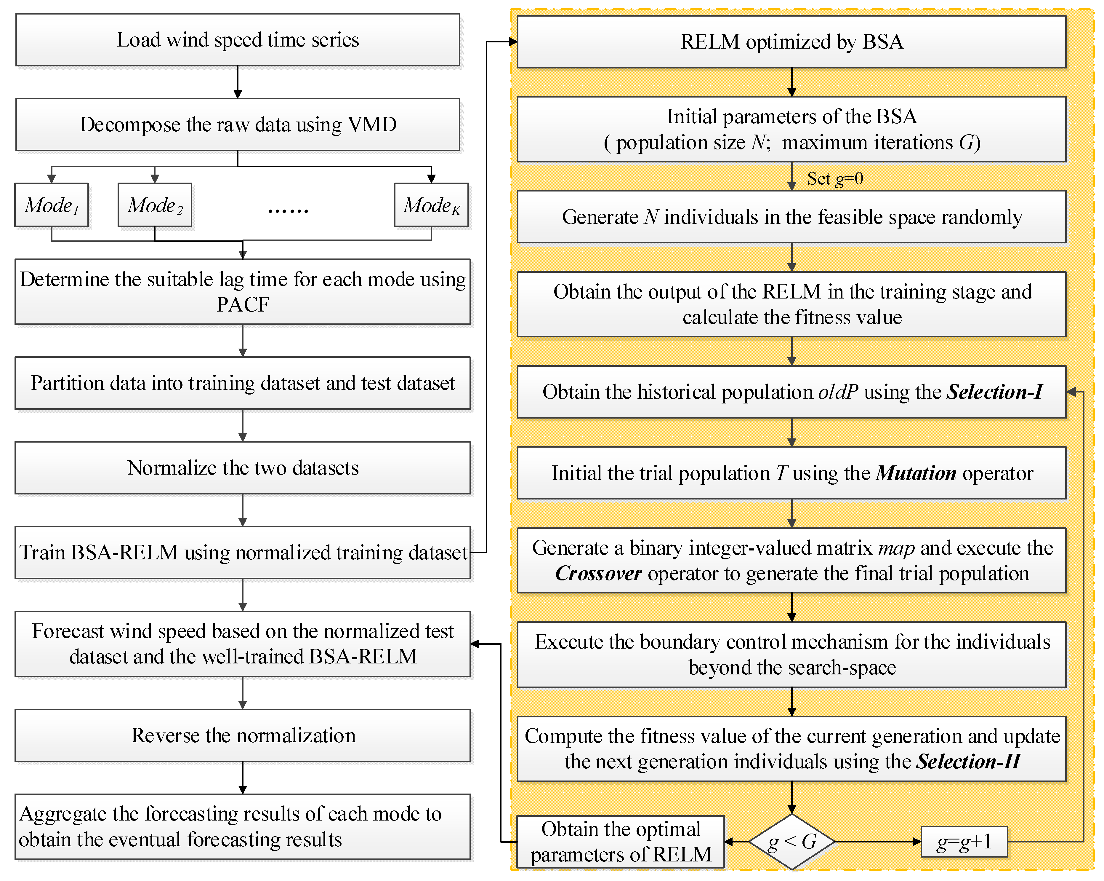
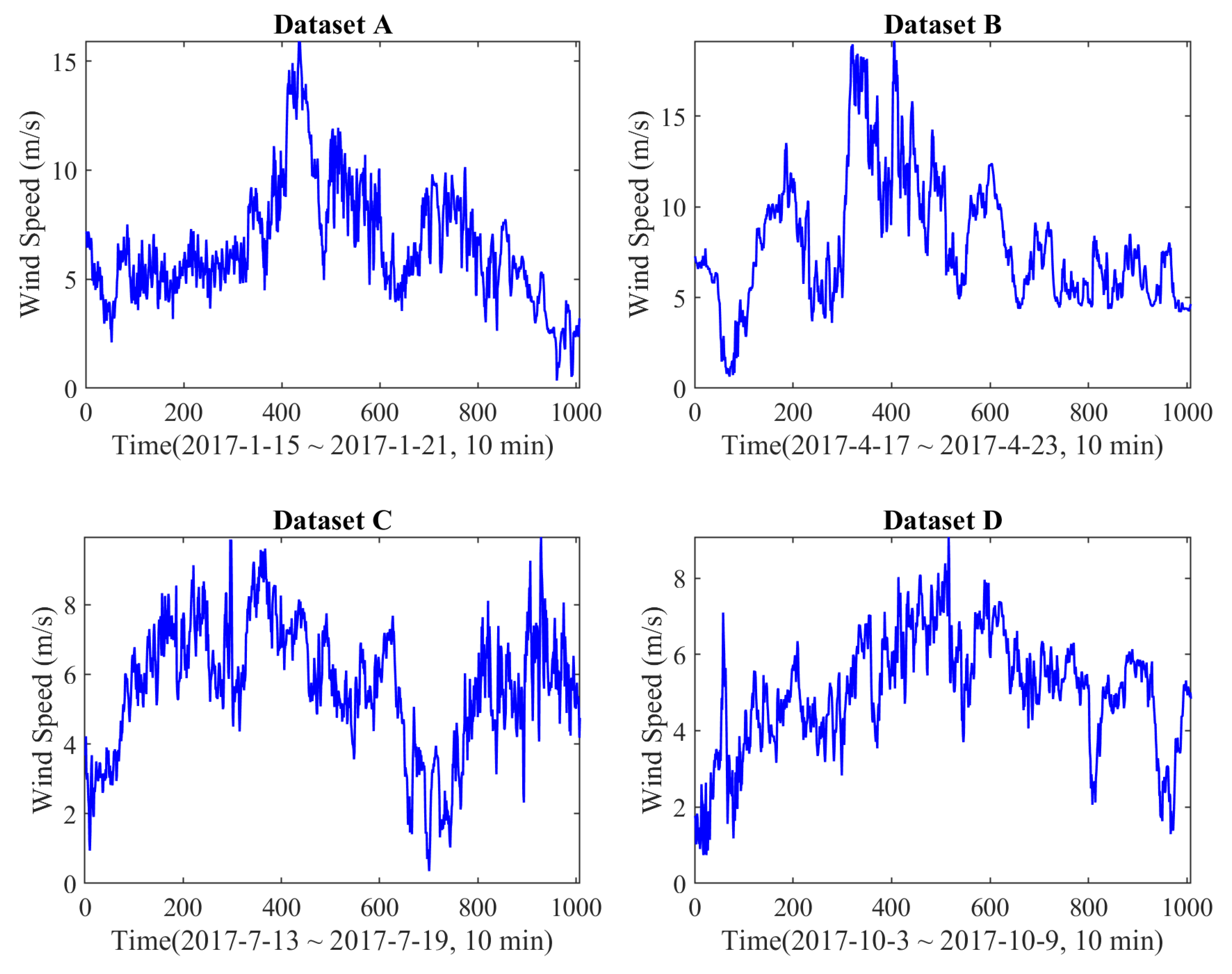
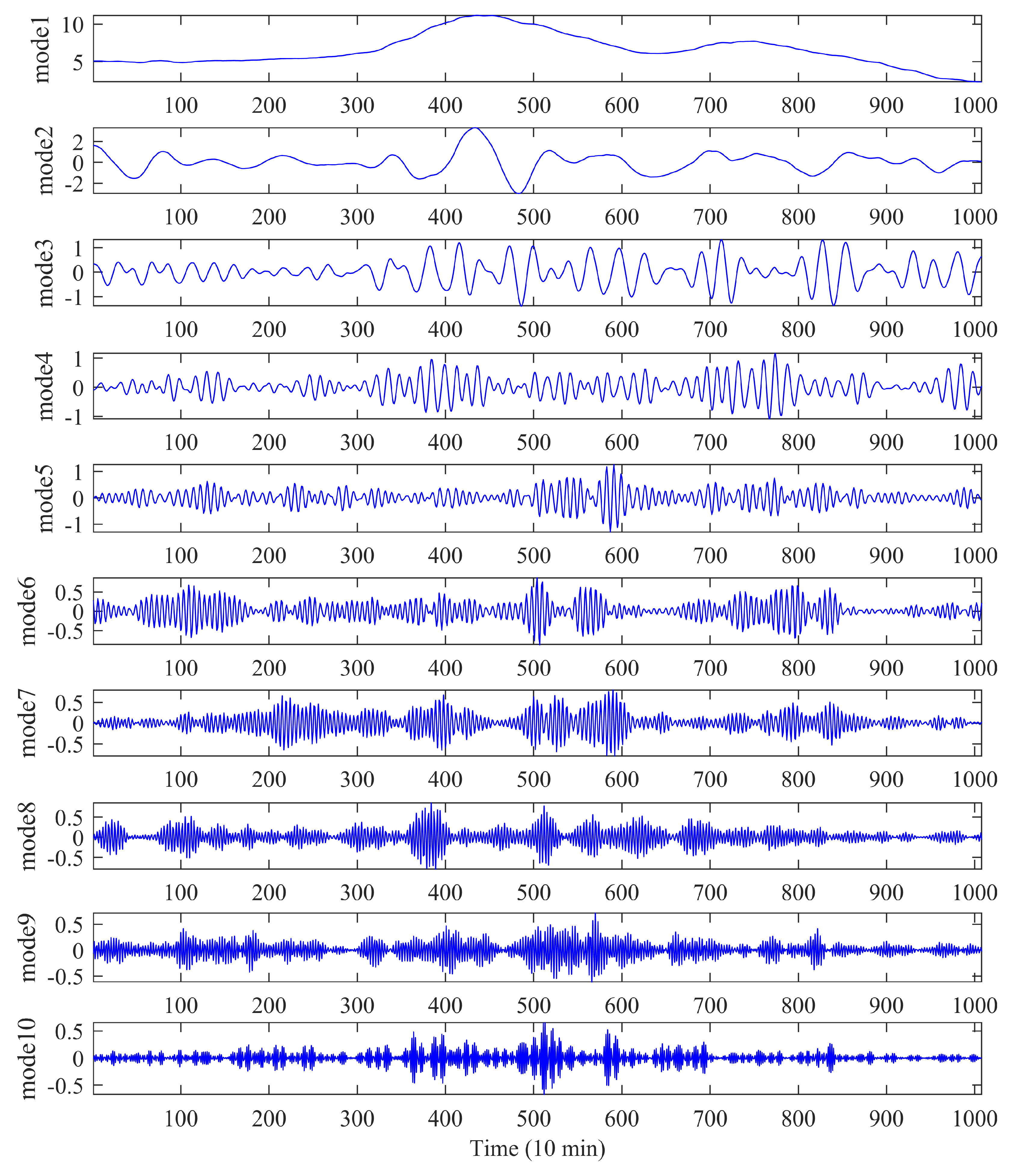
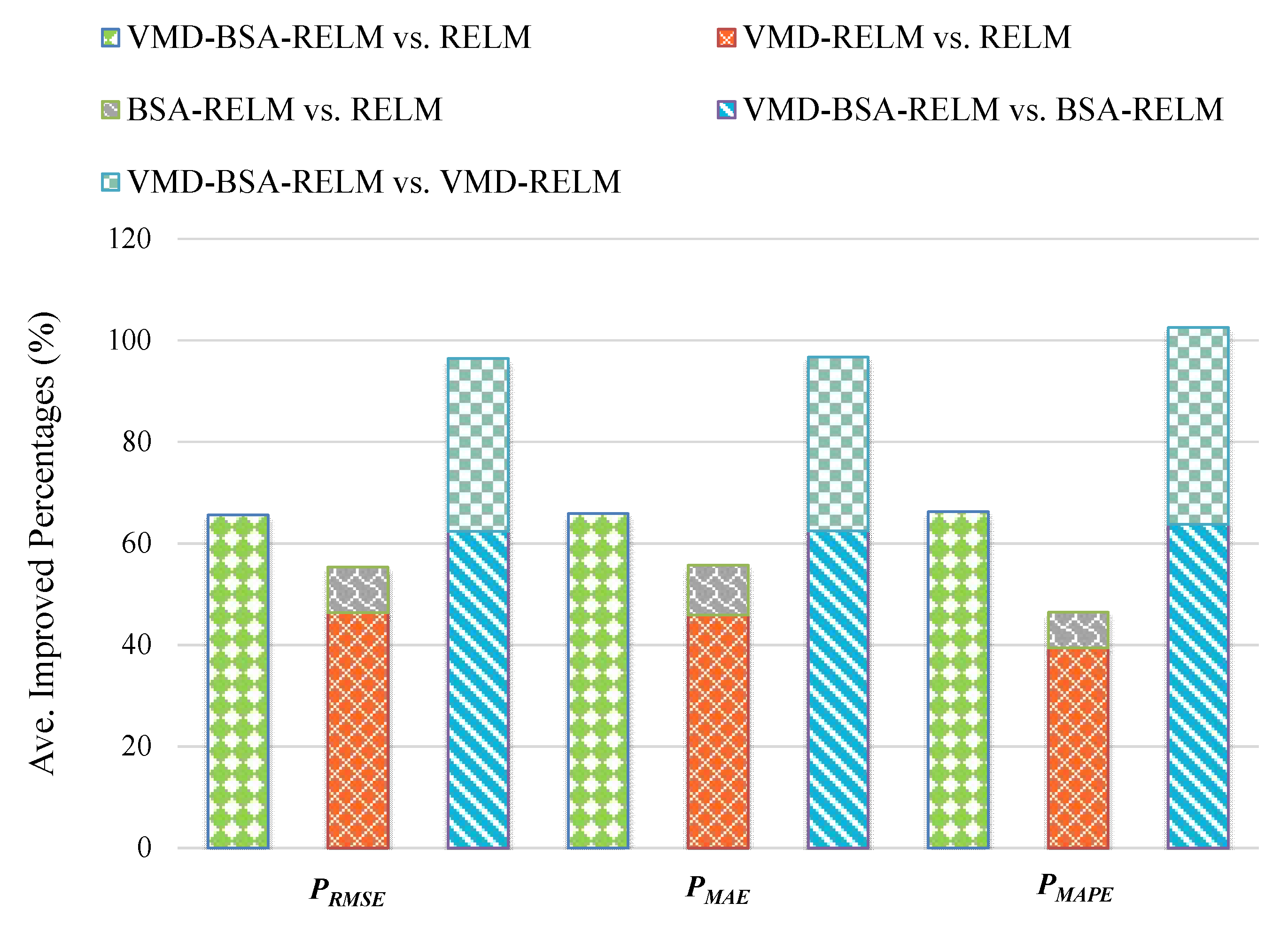
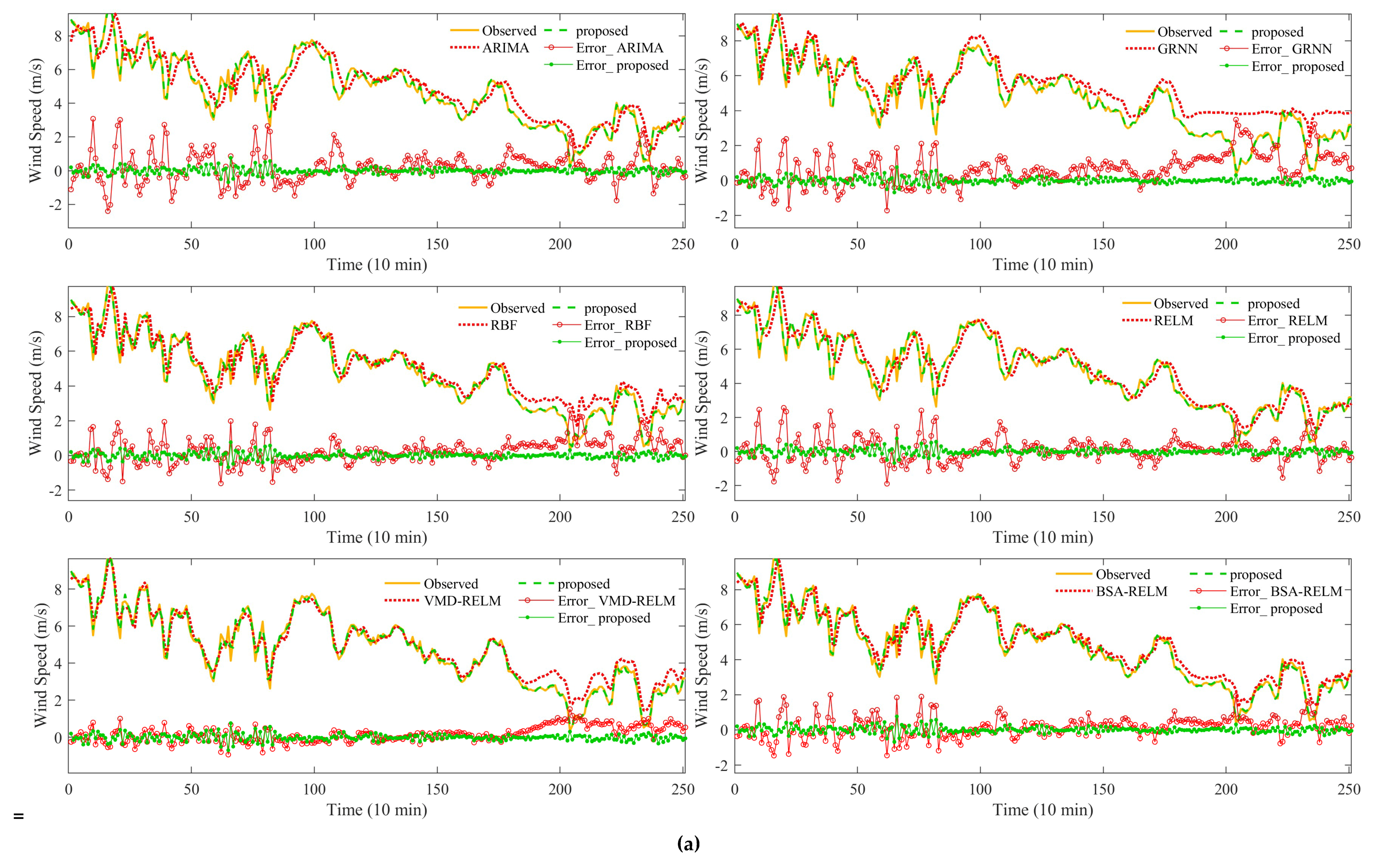
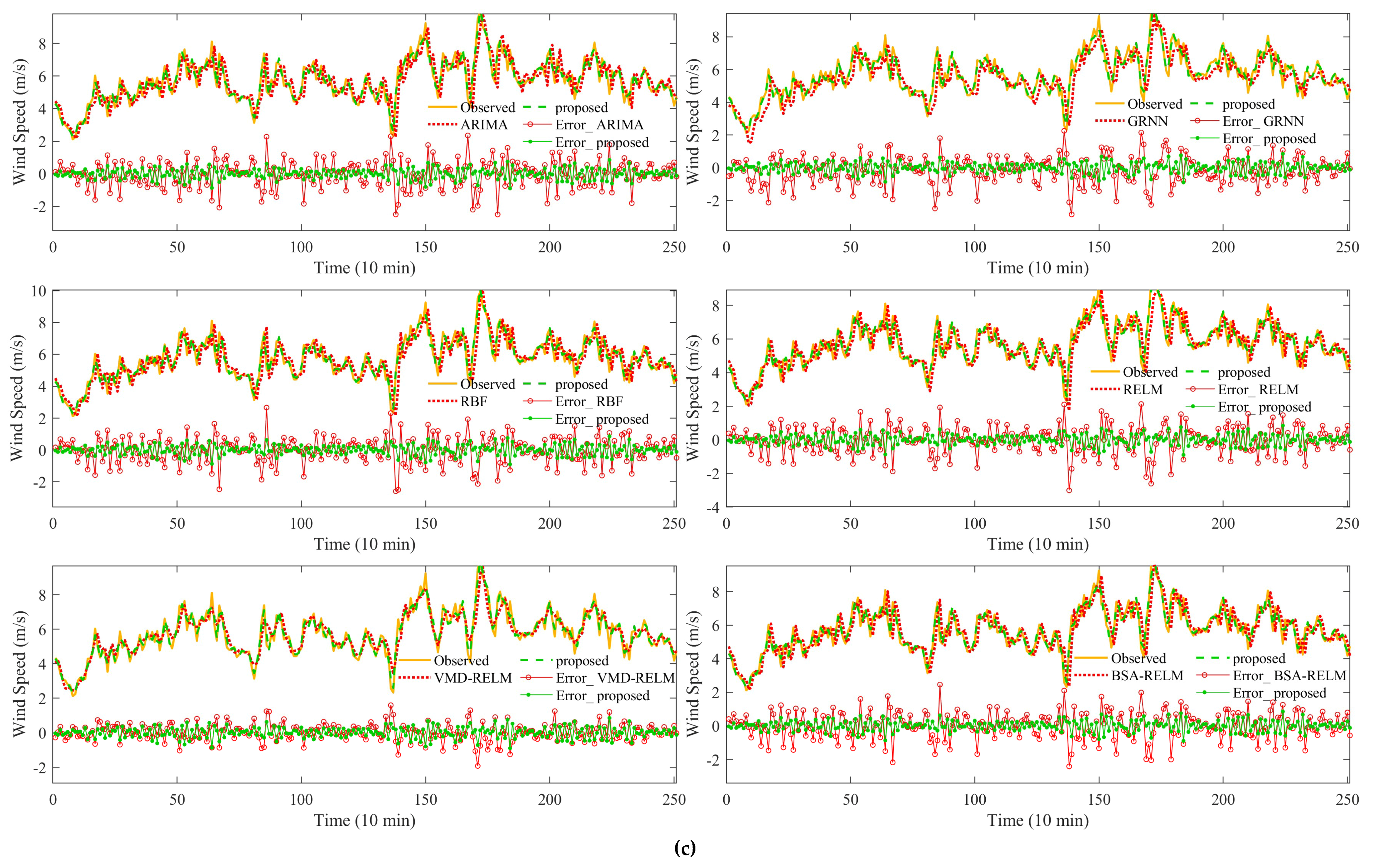
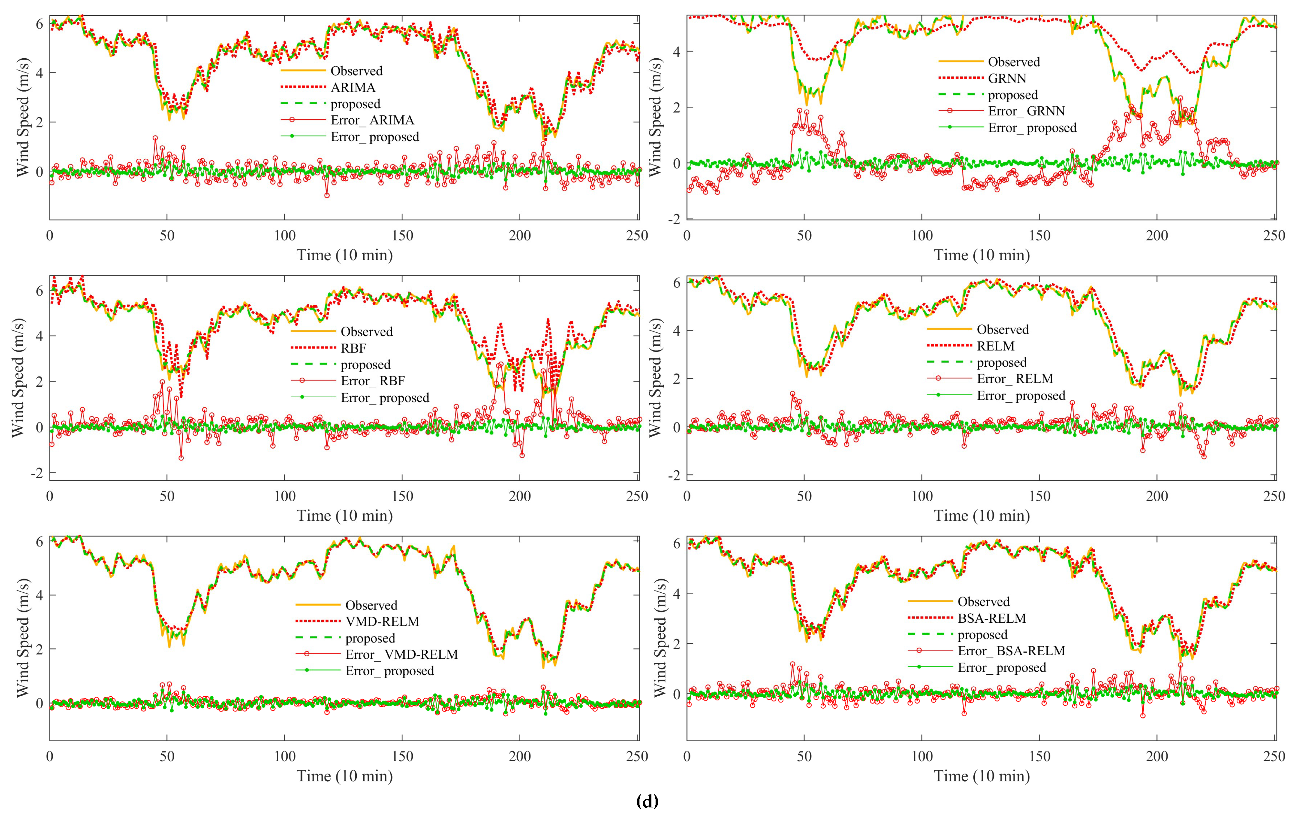
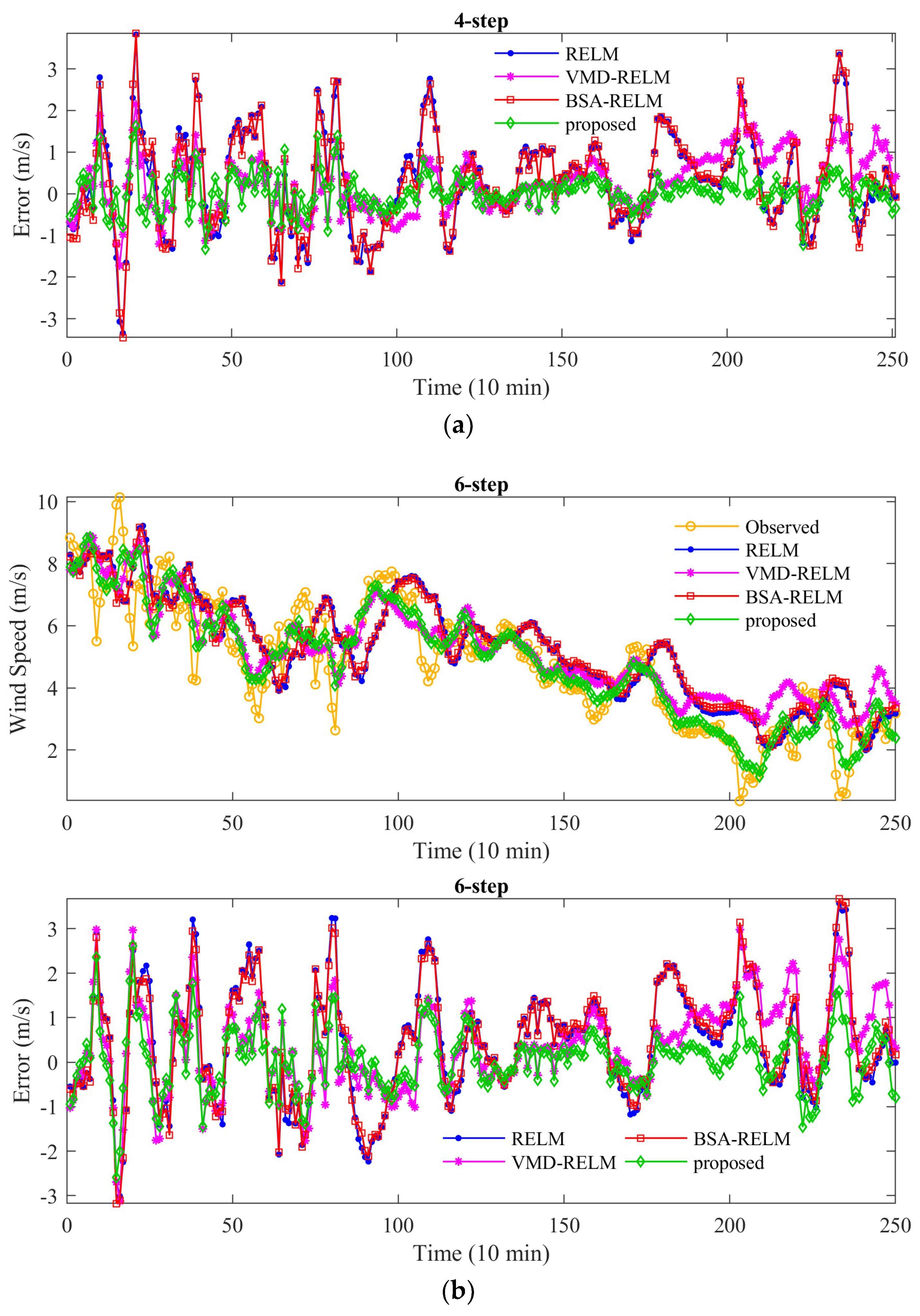
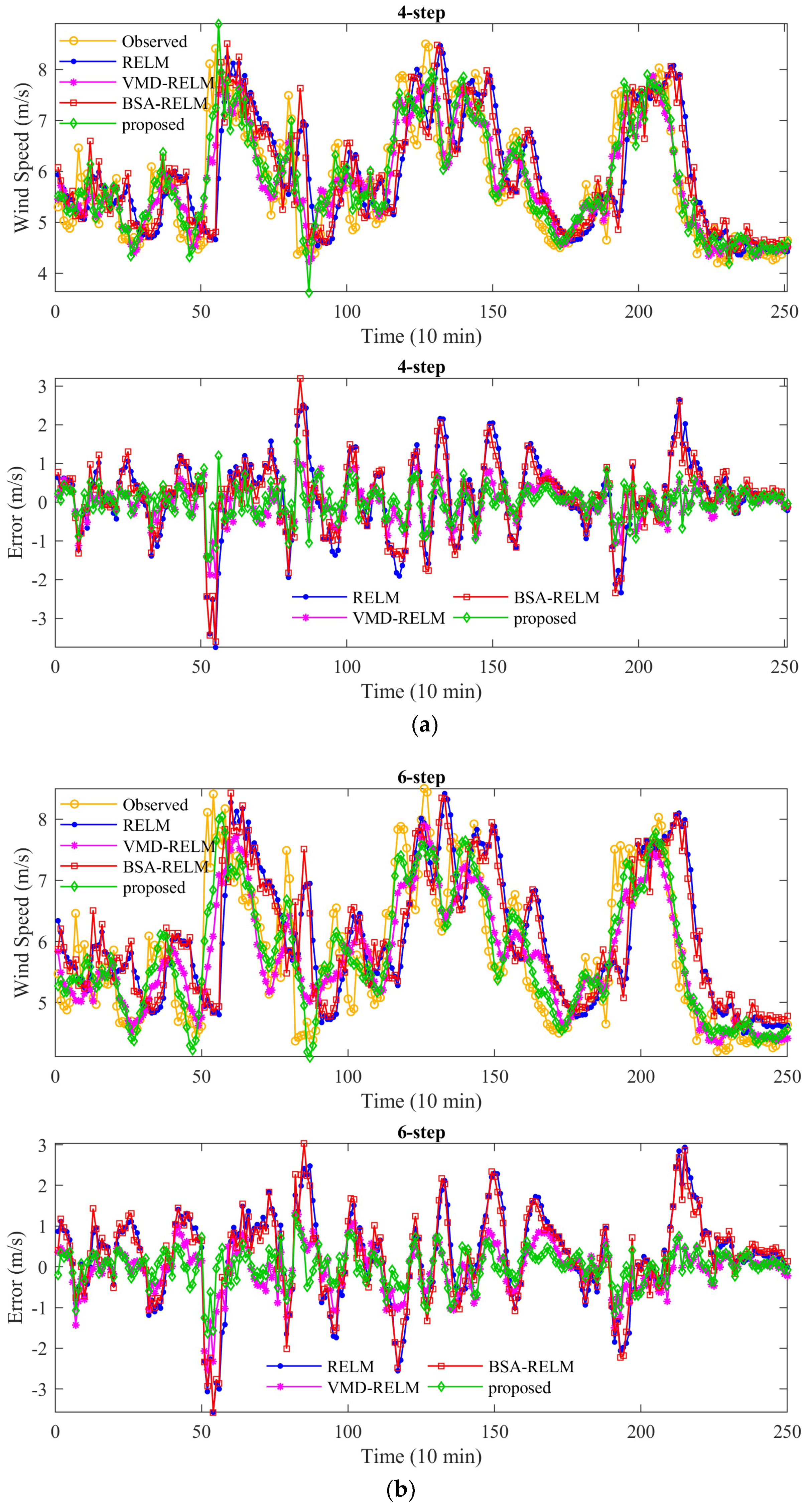
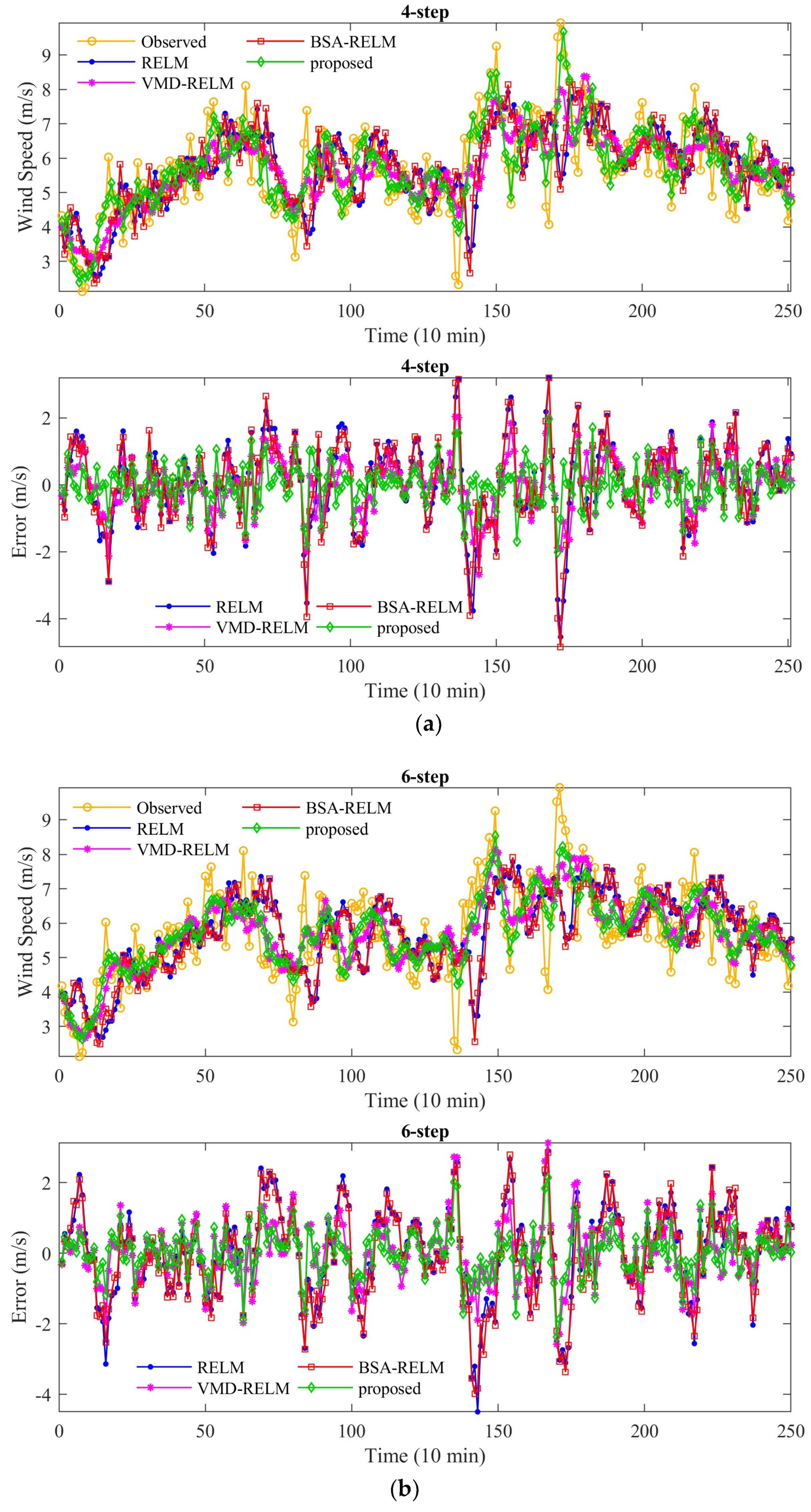
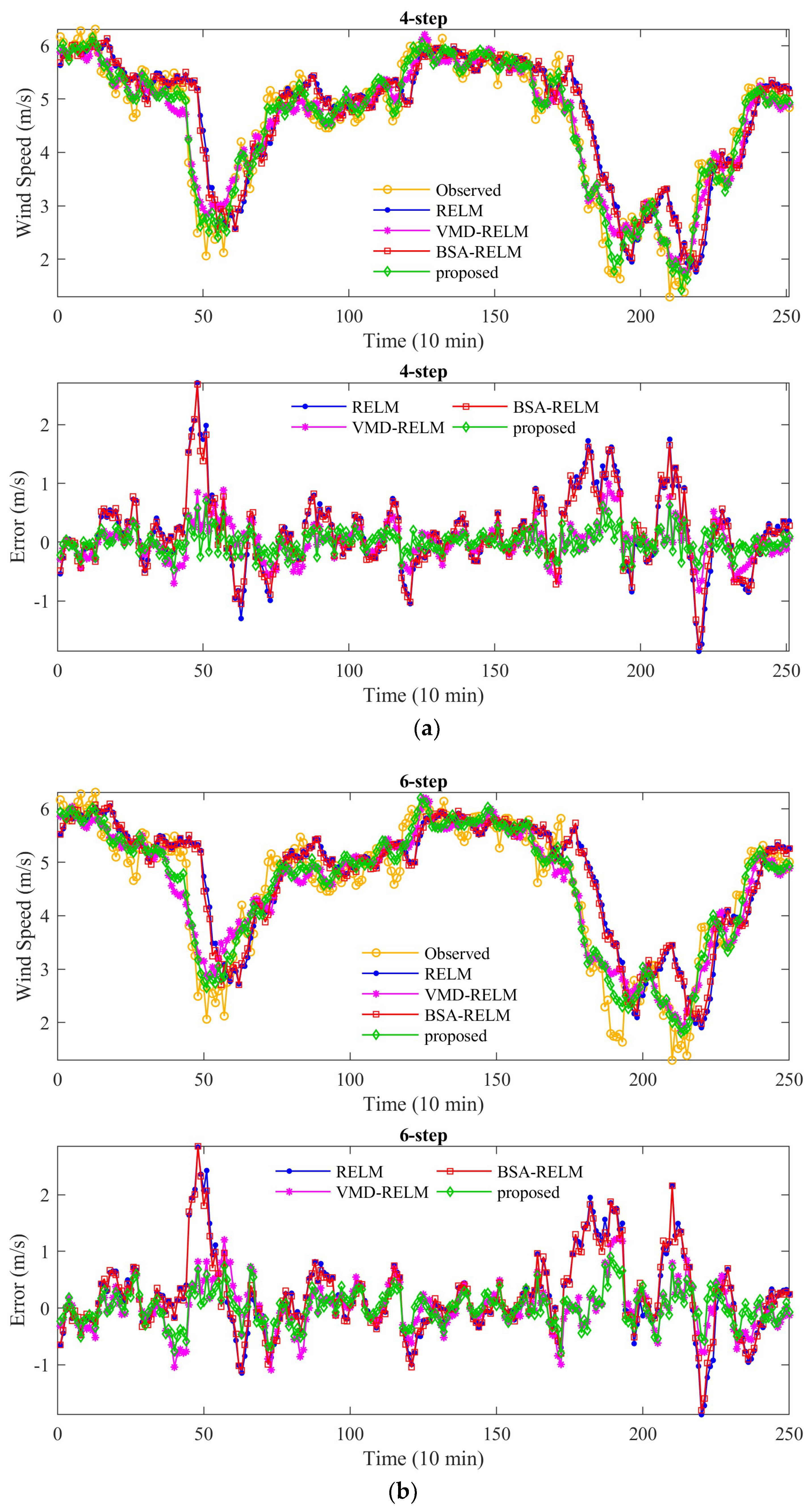
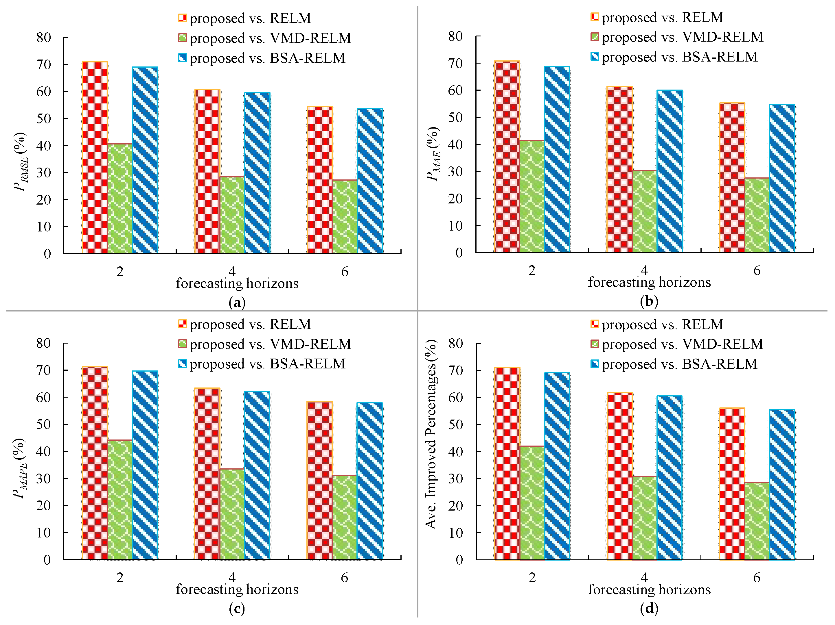
In this study, a novel decomposition-optimization model is proposed through combining RELM, VMD, and BSA to achieve more accurate and reliable ultra-short-term wind speed forecasting. Firstly, VMD is applied to decompose the original wind speed series into a group of relatively stable subseries to reduce the distractions of the randomness and fluctuations of the original series on the prediction accuracy. Then, RELM optimized by BSA is establish to forecast each subseries. Meanwhile, partial autocorrelation function (PACF) is utilized to determine the optimal input vector. Finally, eventual results can be obtained by the aggregation method. To demonstrate the effectiveness of the proposed model, it has been thoroughly tested on several real wind speed datasets from the Sotavento Galicia (SG) wind farm in Spain. Experimental results demonstrate that by using decomposition and optimization techniques together, the forecasting performance of the proposed VMD-BSA-RELM model is significantly better than that of the basic RELM model. Moreover, the decomposition method VMD plays a more important role in the final improvement of the VMD-BSA-RELM model than the optimization method BSA. This clearly shows how important it is to smooth time series to achieve a desired prediction performance.
The main contributions of this study are listed as follows: (a) we first investigate the ability of the combination of VMD, RELM, and BSA to forecast multi-step short-term wind speed; (b) the proposed model can take full advantages of the signal decomposition approach, machine learning, and optimization algorithm; (c) the positive effects of the decomposition and optimization approaches on the final improvement are quantitatively analyzed.
The rest of the paper is organized as follows: the methods involved in the proposed model including VMD, RELM, and BSA are briefly introduced in Section 2; the framework of the proposed decomposition-optimization model is presented in Section 3; experiments and comprehensive analyses to validate the proposed model are presented in Section 4 and Section 5; and Section 6 concludes the paper.

2. Methodology

In this paper, the proposed hybrid model is integrated with three components, variational mode decomposition (VMD), regularized ELM (RELM), and backtracking search algorithm (BSA). So, in this section, separate theories of the VMD-BSA-RELM model will be described in detail.

2.1. Variational Mode Decomposition

Variational mode decomposition (VMD) developed by Dragomiretskiy and Zosso [27] is a novel adaptive and non-recursive signal processing approach. The core of VMD is decomposing a signal f(t) into a series of modes denoted as uk with specific sparsity characteristic [27]. The sparsity of each mode is called its bandwidth in the spectral domain, which can be estimated using the following steps: (1) Employ the Hilbert transform to each mode uk to produce a unilateral frequency spectrum, (2) transform frequency spectrum of each mode to baseband regions by means of an exponential adjusted to the respective estimated frequency, and (3) estimate the bandwidth using the H1 Gaussian smoothness of the demodulated signal, i.e., L2-norm of the gradient. Therefore, the process of decomposition is implemented by settling the following optimization problem:
m i n { u k } , { ω k } { k t [ ( δ ( t ) + j π t ) u k ( t ) ] e j ω k t 2 2 } ,   k = 1 , 2 , , K s . t .   k u k = f ( t )
where u k and w k represent the set of all modes and their frequencies, respectively; f ( t ) denotes the original signal; δ ( t ) denotes the Dirac distribution; and * is convolution operator.
Transform the above optimization problem into an unconstrained one by adding a quadratic penalty term and Lagrangian multipliers, as follows:
L ( { u k } , { ω k } λ ) = α k t [ ( δ ( t ) + j π t ) u k ( t ) ] e j ω k t 2 2 + f ( t ) k u k   2 2 + λ ( t ) , f ( t ) k u k
where α denotes the balancing factor of the data-fidelity constraint.
The above unconstrained optimization problem can be solved by means of the ADMM (alternate direction method of multipliers), which can search the saddle point of the augmented Lagrangian in a series of iterative sub-optimizations by updating u k n + 1 , ω k n + 1 , and λ n + 1 . u k n + 1 , ω k n + 1 , and λ n + 1 are updated by:
u ^ k n + 1 = f ^ ( ω ) i k u ^ i ( ω ) + λ ^ ( ω ) 2 1 + 2 α ( ω ω k ) 2
ω k n + 1 = 0 ω | u ^ k ( ω ) | 2 d ω 0 | u ^ k ( ω ) | 2 d ω
λ ^ n + 1 ( ω ) = λ ^ n ( ω ) + τ ( f ^ ( ω ) i k u ^ k n + 1 ( ω ) )
where u ^ k n + 1 , u ^ i ( ω ) , f ^ ( ω ) , and λ ^ ( ω ) represent the Fourier transform of u k n + 1 , u i ( t ) , f ( t ) , and λ ( t ) , respectively; n denotes the number of iterations; τ is time-step of the dual ascent.
The termination condition of the VMD algorithm is presented as follows:
k u ^ k n + 1 u ^ k n 2 2 / u ^ k n 2 2 < ε
where ε is tolerance of convergence criterion. The entire decomposition process for VMD can be described as:
Step 1:
Initialize parameters for VMD method including u ^ k 1 , ω k 1 , and λ ^ 1 , and set iteration number n = 1.
Step 2:
Calculate u ^ k n + 1 and ω k n + 1 using the Equations (3) and (4).
Step 3:
Update the Lagrangian multiplier in terms of Equation (5) and then set n = n + 1.
Step 4:
Repeat the steps 2–4 until meeting the termination condition. Then, the final decomposed modes can be obtained.

2.2. Regularized Extreme Learning Machine

An extreme learning machine (ELM) is a novel single-hidden-layer feed-forward neural network developed by Huang et al. [16]. The significant feature of an ELM is that it randomly generates the input weights and hidden biases, and then determines its output weights directly according to the Moore-Penrose generalized inverse matrix theory. Suppose there is a given set of training samples ( x t , y t ) with M samples, the output of ELM with L hidden nodes can be estimated by:
y ^ = i = 1 L β i g i ( x ) = i = 1 L β i G ( w i x t + b i )
where g i ( x ) is the activation function of the ith hidden node; w i is the input weight vector; b i is the hidden bias and β i is the output weight connecting the ith hidden node and the output node.
The above equation can be rewritten as:
H β = Y
where β = [ β 1 β L ] T , Y = [ y 1 y M ] T , and H is the hidden layer output matrix defined as :
H = [ h ( x 1 ) h ( x M ) ] = [ G ( ω 1 x 1 + b 1 ) G ( ω L x 1 + b L ) G ( ω 1 x M + b 1 ) G ( ω L x M + b L ) ] M × L
The output weight can be calculated by means of the least squares method to find the optimal solution of the following equation:
min β = H β Y 2
The optimal solution can be written as:
β ^ = H Y
where H is the Moore-Penrose generalized inverse matrix of H, which can be calculated by the following orthogonal projection [16]:
H = [ H T H ] 1 H T
Due to the numerical instability of the pseudo-inverse, the regularized ELM (RELM) is developed through adding a positive value 1 / C into the diagonal elements H T H when calculating the output weights β . Hence, the estimated output weights β ^ of the RELM can be written as:
β ^ = [ H T H + I C ] 1 H T Y
where I is the identity matrix. More information about RELM can be found in [18].

2.3. Backtracking Search Optimization Algorithm

The backtracking search optimization algorithm (BSA), put forward by Civicioglu [32], is a novel stochastic search algorithm for real-valued numerical optimization problems. In contrast to other population-based evolutionary algorithms, BSA has achieved good performance in both computation speed and computation accuracy. The detailed structure of BSA is described as:
(1) Initialization. In this stage, the current population P is randomly generating in the search space by:
P i , j = r a n d ( 0 , 1 ) * ( u p j l o w j ) + l o w j i = 1 , 2 , , N ; j = 1 , 2 , , D ;
where N and D represent the population size and the individual dimensionality, respectively; r a n d ( 0 , 1 ) is a random generator to provide the number in range (0, 1) uniformly.
(2) Selection I. The selection strategy is applied in this process to select the historical population which will guide the search direction in the mutation step. The initial historical population OldP is generated by:
o l d P i , j = r a n d ( 0 , 1 ) * ( u p j l o w j ) + l o w j i = 1 , 2 , , N ; j = 1 , 2 , , D ;
At the beginning of each iteration, the OldP is updated by:
o l d P : = { P ,   a < b p e r m u t i n g ( o l d P ) ,   o t h e r w i s e
where a and b are two random numbers distributed in the range (0, 1) uniformly; p e r m u t i n g ( o l d P ) means that the order of the individuals in oldP is randomly updated by a shuffling function.
(3) Mutation. In this step, the initial form of the trial population Mutant is defined as:
M u t a n t = P + F ( o l d P P ) F = 3 r n d n ,   r n d n ~ N ( 0 , 1 )
where ( o l d P P ) is the search-direction matrix; F is the mutation factor, which controls the amplitude of ( o l d P P ) .
(4) Crossover. In this step, the final form of the trial population T is generated. The crossover operator contains a two-stage process. In the first step, a binary integer-valued matrix map of size N×D is generated by:
{ m a p ( i , u ( 1 : m i x r a t e * r a n d * D ) ) = 0 , w h e n   c < d | c , d ~ U ( 0 , 1 ) m a p ( i , r a n d i ( D ) ) = 0 , o t h e r w i s e
where u = p e r m u t i n g ( D ) represents that the order 1 , 2 , , D is changed by a random shuffle function; mixrate is the only control parameter in BSA (called the mix rate parameter), which controls the number of the individuals that will mutate in a trial.
In the second step, the trial population T is updated by:
T i j = P i j , w h e n   m a p i j = 1 ; i = 1 , 2 , , N ; j = 1 , 2 , , D
Note that, several individuals of the final trial population T may exceed the permissible search space, hence boundary control strategy is quite necessary. The boundary control strategy is:
T i j = r n d ( u p j l o w j ) + l o w j ,   T i j < l o w j   o r   T i j < u p j
(5) Selection II. A greedy selection is applied in this stage to update the population P, trial individuals with better fitness value then are reserved. Steps 2–5 are repeated until the terminal condition is reached.

3. The Proposed Decomposition-Optimization Model

The decomposition-optimization model developed in this study consists of variational mode decomposition (VMD), regularized ELM (RELM), and backtracking search algorithm (BSA). The proposed decomposition-optimization model is shorted as VMD-BSA-RELM. In the VMD-BSA-RELM model, VMD is first used to smooth the wind speed data for preprocessing. RELM is adopted as a predictor. Meanwhile, partial autocorrelation function (PACF) is executed to choose the suitable input vector and BSA is applied to optimize the input weights and hidden thresholds of the RELM model. The detailed procedures of the proposed hybrid VMD-BSA-RELM model are shown in Figure 1.
Due to the multi-step wind speed forecasting can provide more useful information for decision makers, so the proposed VMD-BSA-RELM model is executed for multi-step wind speed forecasting. The input-output combinations for different forecasting horizons are shown as:
y ^ t + h = f ( y t 1 , y t 2 , , y t d )
where h is forecasting horizon; d is the suitable lag time which is determined by the PACF.

4. Experimental Design

4.1. Data Collection

In this study, historical wind speed data were collected from the Sotavento Galicia (SG) wind farm (original wind speed data from the SG wind farm can be found at: http://sotaventogalicia.com/en/real-time-data/historical.). The SG wind farm is located in Galicia, in northwest Spain, with latitude/longitude of 43.354377° N and 7.881213° W. Considering the influence of seasonal factors on forecasting accuracy, four datasets, A, B, C, and D, from different seasons were selected to verify the effectiveness of the proposed VMD-BSA-RELM method. Time periods of the four datasets are 15–21 January, 17–23 April, 13–19 July, and 3–9 October, respectively. Each dataset includes 1008 points with 10 min interval. Based on our test results and [36,37,38,39], in each dataset, the first 75% data are selected as training samples to build the prediction model while the remaining 25% are utilized to test. The proposed model is applied to obtain 1-step, 2-step, 4-step, and 6-step (1 h) ahead wind speed forecasting. The raw wind speed data are shown in Figure 2, which indicates non-stationary and nonlinear features of wind speed series.
The statistical information including average (Ave.) value, maximum (Max.) value, minimum (Min.) value, standard deviation (Std.), the coefficient of variation (Cv) and the skewness coefficient (Cs) of the four datasets are listed in Table 1. The standard deviations of all datasets are all above 1.49 (m/s), and the maximum/minimum values of Datasets A-D are 15.91/0.35 (m/s), 19.13/0.64 (m/s), 9.94/0.35 (m/s), and 9.08/0.74 (m/s). These results also indicate the non-stationary and nonlinear features of the original wind speed series.

4.2. Data Decomposition and Parameters Settings

VMD is executed to decompose the raw wind speed series into several relatively stable modes to make them easy to be predicted. Before the implementation of the decomposition using VMD, the number of modes K needs to be preset. In this study, number of modes for each wind speed series is searched in the range [3,14], respectively. Then, the suitable number of modes is determined by the center pulsation of the decomposed modes [19]. After that, each mode will be forecasted by the RELM optimized by BSA (BSA-RELM for short). The input vector of the BSA-RELM is determined by the partial autocorrelation function (PACF). Take Dataset A as an example, the subseries generated by VMD are shown in Figure 3 and the PACF values with 95% confidence interval are presented in Figure 4. According to the partial autocorrelograms in Figure 4, the lagged variable with PACF value over the confidence interval will be chosen to form the input vector of forecasting model. The population size and the maximum iterations of BSA are set to 50 and 100, respectively. The input selection approach PACF is exploited for all forecasting models involved in this study to guarantee fair and effective comparisons.

4.3. Evaluation Indices

To evaluate forecasting performance of all forecasting models, three commonly used error evaluation metrics including mean absolute error (MAE), mean absolute percent error (MAPE), and root mean square error (RMSE) are used in the study. They can be calculated by:
R M S E = 1 N i = 1 N ( y i y ^ i ) 2
M A P E = 1 N i = 1 N | y i y ^ i y i |
M A E = 1 N i = 1 N | y i y ^ i |
where y i and y ^ i are the ith observed and predicted wind speed, respectively; N is the number of samples.
To clearly view the improvement of a specific model, improved percentage metrics of RMSE, MAE, and MAPE including PMAE, PRMSE, and PMAPE are calculated to exhibit the relative improvement degree between two different models denoted as Model 1 and Model 2. PMAE, PRMSE, and PMAPE of Model 2 relative to Mode 1 can be defined as:
P M A E = 100 × ( M A E 1 M A E 2 ) / M A E 1
P R M S E = 100 × ( R M S E 1 R M S E 2 ) / R M S E 1
P M A P E = 100 × ( M A P E 1 M A P E 2 ) / M A P E 1

5. Results and Discussions

Several experimental results are presented in this section to demonstrate the efficiency and applicability of the proposed decomposition-optimization model (VMD-BSA-RELM). These experiments are grouped into three subsections: one-step forecasting results, multi-step forecasting results, and Diebold-Mariano tests and computational time.

5.1. One-Step Forecasting Results

This part focuses on presenting the one-step forecasting performance of the proposed VMD-BSA-RELM forecasting model using four datasets from different seasons. ARIMA, RBF, GRNN, RELM, VMD-RELM, and BSA-RELM are used as comparison models. Akaike’s Information Criteria (AIC), which has widely used in model selections [40,41], is used to determine the appropriate parameters of ARIMA. RMSE, MAE, and MAPE values provided by these seven forecasting models on the testing data for all datasets are exhibited in Table 2, where the model with the lowest evaluation indices values are highlighted in green. It can be seen that as for the three single neural network models (RELM, GRNN, and RBF), RELM has the best performance and GRNN has the worst performance for all datasets from different seasons. Meanwhile, forecasting results of ARIMA are closer to that of RELM in some cases. Further, comparisons of RELM and VMD-RELM, RELM and BSA-RELM, RELM and VMD-BSA-RELM suggest hybrid models outperform single model in all cases. This can be directly and clearly seen in Table 3 and Figure 5. It is clear that both VMD and BSA have positive effects on improving forecasting accuracy, while BSA has less contribution than VMD. Figure 5 visually indicates that the decomposition-optimization method can gain remarkable improvement of forecasting accuracy compared with hybrid models based on either signal decomposition approach or optimization algorithm. This clearly shows how important it is to incorporate VMD, BSA, and RELM to achieve a desired prediction performance. Concretely, the average improved percentages of RMSE, MAE, and MAPE between the VMD-BSA-RELM model and the single RELM model are 65.60%, 65.88%, and 66.21%, respectively, indicating a remarkable improvement. Figure 5 also shows that PRMSE, PMAE, and PMAPE values between VMD-BSA-RELM and VMD-RELM are greater than those between VMD-RELM and RELM. Similarly, PRMSE, PMAE, and PMAPE values between VMD-BSA-RELM and BSA-RELM are greater than those between BSA-RELM and RELM. These results emphasize the importance of the signal decomposition approach VMD, and the proposed models can take full advantages of both decomposition and optimization techniques. Predicted and observed curves as well as forecasting errors of all forecasting models are shown in Figure 6, where the predicted curves of the VMD-BSA-RELM model are close to real curves and its forecasting errors are evenly distributed around zero with a tiny range.

5.2. Multi-Step Forecasting Results

This section is devoted to illustrate the efficacy of the proposed model on multi-step wind speed forecasting. The RELM, VMD-RELM, and BSA-RELM which perform better among all competitors are performed as benchmark models in this experiment. Table 4 displays the forecasting performance for different seasons by these four models in 2-step, 4-step, and 6-step forecasting in terms of RMSE, MAE, and MAPE values, where the lowest values among diverse models are emphasized in green. It can be seen that although the forecasting performances deteriorate as the length of the forecasting horizons increase, the proposed model can always outperform than other forecasting models in all cases and horizons, followed by the VMD-RELM model, last the RELM. For instance, for the Dataset A (Winter), the RMSE value of the proposed model (VMD-BSA-RELM) in 2-step, 4-step, and 6-step are 0.2462 m/s, 0.4286 m/s, and 0.7120 m/s, respectively, which are better than these of 0.604 m/s, 0.7544 m/s and 1.0633 m/s for VMD-RELM. Moreover, the performance of BSA-RELM is closer to or even worse than that of the RELM along with the increase of the forecasting steps. More concretely, for the Dataset C, the RMSE and MAE values of the BSA-RELM are 1.2911 m/s and 1.0298 m/s for 6-step forecasting, which are slightly worse than these of 1.2893 m/s and 1.0286 m/s for the single RELM model.
The 4-step and 6-step wind speed forecasting results as well as forecasting errors for different models are presented in Figure 7, Figure 8, Figure 9 and Figure 10, where the superiority of the VMD-BSA-RELM model is confirmed. In these figures, the proposed VMD-BSA-RELM model always provides the smallest forecasting error variation ranges than other models and can accurately capture the variation trend of real wind speed, even for the 6-step forecasting. Additionally, forecasting errors increase along with the growth of horizons, specifically in peak and valley parts. Overall, the proposed model can maximize the advantages of the VMD and BSA methods to produce highly accurate results in multi-step forecasting, which is consistent with the conclusion drawn from one-step forecasting results.
The improved percentages of the proposed VMD-BSA-RELM model on the basis of RELM, VMD-RELM, and BSA-RELM for multi-step forecasting results are tabulated in Table 5. To visually view the improvements, the average improved percentages for different forecasting horizons in the last three rows of Table 5 are exhibited in Figure 11, where remarkable improvements of the proposed model over its competitors on all three metrics are revealed. The average improved ratios of all horizons for RELM, VMD-RELM, and BSA-ELM are 62.9%, 33.74%, and 61.63%, respectively. In summary, according to Table 3 and Table 5, the proposed model produces a better result with a least 53.63% average improved ratios over three competitors with better performance among all benchmark models (RELM, VMD-RELM, and BSA-RELM) under all datasets and all horizons (1-, 2-, 4- and 6-step).

5.3. Diebold-Mariano Tests and Computational Time

In this part, the Diebold-Mariano (DM) test [42] is applied to assess whether there are real differences between the proposed model and its competitors. The DM test results calculated by the square error loss function are tabulated in Table 6. It can be seen that the DM statistical values of the RELM, VMD-RELM, and BSA-RELM are more than the threshold value of the 1% significance level for all datasets and all forecasting horizons, which demonstrates the proposed model is superior to its rivals.
The average values of computational times of various step-ahead wind speed forecasting, with regard to Datasets A, B, C, and D, for all prediction models, are shown in Table 7. When compared with the other forecasting models, the proposed VMD-BSA-RELM model has higher time consumption due to the utilization of the optimization algorithm BSA, whereas its computational time is acceptable in real engineering application. These results have proven that the VMD-BSA-RELM model can provide more accurate wind speed forecasting results through sacrificing computational time within an admissible degree.

6. Conclusions

Wind speed forecasting is a crucial part of wind energy generation. However, due to its inherent randomness, high non-linearity and non-stationarity, accurate wind speed forecasting is a very challengeable task. In this study, a new decomposition-optimization method called VMD-BSA-RELM is proposed for short-term wind speed forecasting. Original wind speed data is preprocessed by VMD into a group of relative stationary modes where regressions by RELM are executed. Suitable parameters of RELMs are determined by means of BSA. The efficacy of the VMD-BSA-RELM was tested against several benchmark models using several datasets under different forecasting horizons. The results indicate that the VMD-BSA-RELM model significantly outperforms the other models and sacrifices computational time with an acceptable degree in real applications. Additionally, quantitative analyses of the effects of decomposition and optimization techniques on the final improvement of forecasting accuracy show that the decomposition approach, VMD, contributes more than the optimization method, BSA. The VMD-BSA-RELM combines VMD with BSA and thus take full advantages of both two methods. In conclusion, the proposed method is a powerful tool in short-term wind speed forecasting. Future work will focus on the investigation of the maximum forecasting horizons of the VMD-BSA-RELM model and introducing error correct techniques to improve its accuracy in large multi-step forecasting, especially in peak and valley parts.

Author Contributions

J.Z. and N.S. designed and performed the model simulation; N.S. wrote the draft of the paper; B.J. prepared the figures in the revised paper; T.P. polished the manuscript.

Funding

This research is funded by the National Natural Science Foundation of China (Nos. 91547208, 51579107, 91647114), and the National Key R&D Program of China (No. 2017YFC0405900).

Acknowledgments

This work is supported by the National Natural Science Foundation of China (Nos. 91547208, 51579107, 91647114), and the National Key R&D Program of China (No. 2017YFC0405900).

Conflicts of Interest

The authors declare no conflict of interest.

Nomenclature

u k All modes of VMD
w k Frequencies of all modes
f ( t ) Original signal
δ ( t ) Dirac distribution
α The balancing parameter of the data-fidelity constraint
u ^ k n + 1 Fourier transform of u k n + 1
u ^ i ( ω ) Fourier transform of u i ( t )
f ^ ( ω ) Fourier transform of f ( t )
λ ^ ( ω ) Fourier transform of u i ( t )
τ Time-step of the dual ascent
ε Tolerance of convergence criterion
g i ( x ) Activation function
w i The input weight vector
H The hidden layer output matrix
H Moore-Penrose generalized inverse matrix of H
( x t , y t ) Training samples
MTotal number of training samples
Lhidden nodes
NPopulation size
DIndividual dimensionality
a, bRandom numbers distributed uniformly from 0 to 1
OldPHistorical population
TTrial population
PCurrent population
mixrateMix rate parameter of BSA
hForecasting horizon
dSuitable lag time

References

  1. Global Wind Energy Council (GWEC). Global Wind Report 2016-Annual Market Update; GWEC: Brussels, Belgium, 2016. [Google Scholar]
  2. Soman, S.S.; Zareipour, H.; Malik, O.; Mandal, P. A review of wind power and wind speed forecasting methods with different time horizons. In Proceedings of the 2010 North American Power Symposium, Arlington, TX, USA, 26–28 September 2010; pp. 1–8. [Google Scholar]
  3. Weron, R. Electricity price forecasting: A review of the state-of-the-art with a look into the future. Int. J. Forecast. 2014, 30, 1030–1081. [Google Scholar] [CrossRef]
  4. Sun, N.; Zhou, J.Z.; Zhu, S.; Wei, L.I.; Peng, T. Application of Hybrid Models Based on Wavelet Analysis and Two Different Neural Networks in Prediction of Monthly Runoff. Water Resour. Power 2018. [Google Scholar] [CrossRef]
  5. Sun, N.; Zhou, J. Non-stationary runoff hybrid forecasting model based on regularized extreme learning machine. J. Hydroel. Eng. 2018, 1, 1–9. [Google Scholar]
  6. Cincotti, S.; Gallo, G.; Ponta, L.; Raberto, M. Modeling and forecasting of electricity spot-prices: Computational intelligence vs. classical econometrics. Ai Commun. 2014, 27, 301–314. [Google Scholar]
  7. Lydia, M.; Kumar, S.S.; Selvakumar, A.I.; Kumar, G.E.P. Linear and non-linear autoregressive models for short-term wind speed forecasting. Energy Convers. Manag. 2016, 112, 115–124. [Google Scholar] [CrossRef]
  8. Han, Q.; Meng, F.; Hu, T.; Chu, F. Non-parametric hybrid models for wind speed forecasting. Energy Convers. Manag. 2017, 148, 554–568. [Google Scholar] [CrossRef]
  9. Wang, J.; Hu, J. A robust combination approach for short-term wind speed forecasting and analysis–Combination of the ARIMA (Autoregressive Integrated Moving Average), ELM (Extreme Learning Machine), SVM (Support Vector Machine) and LSSVM (Least Square SVM) forecasts using a GPR (Gaussian Process Regression) model. Energy 2015, 93, 41–56. [Google Scholar]
  10. Liu, H.; Tian, H.; Liang, X.; Li, Y. New wind speed forecasting approaches using fast ensemble empirical model decomposition, genetic algorithm, mind evolutionary algorithm and artificial neural networks. Renew. Energy 2015, 83, 1066–1075. [Google Scholar] [CrossRef]
  11. Ren, C.; An, N.; Wang, J.; Li, L.; Hu, B.; Shang, D. Optimal parameters selection for BP neural network based on particle swarm optimization: A case study of wind speed forecasting. Knowl.-Based Syst. 2014, 56, 226–239. [Google Scholar] [CrossRef]
  12. Wang, S.; Zhang, N.; Wu, L.; Wang, Y. Wind speed forecasting based on the hybrid ensemble empirical mode decomposition and GA-BP neural network method. Renew. Energy 2016, 94, 629–636. [Google Scholar] [CrossRef]
  13. Wang, J.; Heng, J.; Xiao, L.; Wang, C. Research and application of a combined model based on multi-objective optimization for multi-step ahead wind speed forecasting. Energy 2017, 125, 591–613. [Google Scholar] [CrossRef]
  14. Wang, J.; Yang, W.; Du, P.; Li, Y. Research and application of a hybrid forecasting framework based on multi-objective optimization for electrical power system. Energy 2018, 148, 59–78. [Google Scholar] [CrossRef]
  15. Yu, C.; Li, Y.; Zhang, M. An improved Wavelet Transform using Singular Spectrum Analysis for wind speed forecasting based on Elman Neural Network. Energy Convers. Manag. 2017, 148, 895–904. [Google Scholar] [CrossRef]
  16. Huang, G.B.; Zhu, Q.Y.; Siew, C.K. Extreme learning machine: Theory and applications. Neurocomputing 2006, 70, 489–501. [Google Scholar] [CrossRef] [Green Version]
  17. MartíNez-MartíNez, J.M.; Escandell-Montero, P.; Soria-Olivas, E.; MartíN-Guerrero, J.D.; Magdalena-Benedito, R.; GóMez-Sanchis, J. Regularized extreme learning machine for regression problems. Neurocomputing 2011, 74, 3716–3721. [Google Scholar] [CrossRef]
  18. Chen, K.; Lv, Q.; Lu, Y.; Dou, Y. Robust regularized extreme learning machine for regression using iteratively reweighted least squares. Neurocomputing 2017, 230, 345–358. [Google Scholar] [CrossRef]
  19. Huang, N.; Yuan, C.; Cai, G.; Xing, E. Hybrid Short Term Wind Speed Forecasting Using Variational Mode Decomposition and a Weighted Regularized Extreme Learning Machine. Energies 2016, 9, 989. [Google Scholar] [CrossRef]
  20. Shao, H.; Deng, X.; Cui, F. Short-term wind speed forecasting using the wavelet decomposition and AdaBoost technique in wind farm of East China. Iet Gener. Transm. Distrib. 2016, 10, 2585–2592. [Google Scholar] [CrossRef]
  21. Liu, D.; Niu, D.; Wang, H.; Fan, L. Short-term wind speed forecasting using wavelet transform and support vector machines optimized by genetic algorithm. Renew. Energy 2014, 62, 592–597. [Google Scholar] [CrossRef]
  22. Wang, Y.; Wu, L. On practical challenges of decomposition-based hybrid forecasting algorithms for wind speed and solar irradiation. Energy 2016, 112, 208–220. [Google Scholar] [CrossRef]
  23. Guo, Z.; Zhao, W.; Lu, H.; Wang, J. Multi-step forecasting for wind speed using a modified EMD-based artificial neural network model. Renew. Energy 2012, 37, 241–249. [Google Scholar] [CrossRef]
  24. Yu, C.; Li, Y.; Zhang, M. Comparative study on three new hybrid models using Elman Neural Network and Empirical Mode Decomposition based technologies improved by Singular Spectrum Analysis for hour-ahead wind speed forecasting. Energy Convers. Manag. 2017, 147, 75–85. [Google Scholar] [CrossRef]
  25. Abdoos, A.A. A new intelligent method based on combination of VMD and ELM for short term wind power forecasting. Neurocomputing 2016, 203, 111–120. [Google Scholar] [CrossRef]
  26. Zhang, Y.; Liu, K.; Qin, L.; An, X. Deterministic and probabilistic interval prediction for short-term wind power generation based on variational mode decomposition and machine learning methods. Energy Convers. Manag. 2016, 112, 208–219. [Google Scholar] [CrossRef]
  27. Dragomiretskiy, K.; Zosso, D. Variational Mode Decomposition. IEEE Transac. Signal Process. 2014, 62, 531–544. [Google Scholar] [CrossRef]
  28. Gao, Y.; Qu, C.; Zhang, K. A Hybrid Method Based on Singular Spectrum Analysis, Firefly Algorithm, and BP Neural Network for Short-Term Wind Speed Forecasting. Energies 2016, 9, 757. [Google Scholar] [CrossRef]
  29. Yin, H.; Dong, Z.; Chen, Y.; Ge, J.; Lai, L.L.; Vaccaro, A.; Meng, A. An effective secondary decomposition approach for wind power forecasting using extreme learning machine trained by crisscross optimization. Energy Convers. Manag. 2017, 150, 108–121. [Google Scholar] [CrossRef]
  30. Yuan, X.; Chen, C.; Yuan, Y.; Huang, Y.; Tan, Q. Short-term wind power prediction based on LSSVM–GSA model. Energy Convers. Manag. 2015, 101, 393–401. [Google Scholar] [CrossRef]
  31. Osório, G.; Matias, J.; Catalão, J. Short-term wind power forecasting using adaptive neuro-fuzzy inference system combined with evolutionary particle swarm optimization, wavelet transform and mutual information. Renew. Energy 2015, 75, 301–307. [Google Scholar] [CrossRef]
  32. Civicioglu, P. Backtracking Search Optimization Algorithm for numerical optimization problems. Appl. Math. Comput. 2013, 219, 8121–8144. [Google Scholar] [CrossRef]
  33. Zhang, C.; Zhou, J.; Li, C.; Fu, W.; Peng, T. A compound structure of ELM based on feature selection and parameter optimization using hybrid backtracking search algorithm for wind speed forecasting. Energy Convers. Manag. 2017, 143, 360–376. [Google Scholar] [CrossRef]
  34. Taslimi-Renani, E.; Modiri-Delshad, M.; Elias, M.F.M.; Rahim, N.A. Development of an enhanced parametric model for wind turbine power curve. Appl. Energy 2016, 177, 544–552. [Google Scholar] [CrossRef]
  35. Renani, E.T.; Elias, M.F.M.; Rahim, N.A. Using data-driven approach for wind power prediction: A comparative study. Energy Convers. Manag. 2016, 118, 193–203. [Google Scholar] [CrossRef]
  36. Xiao, L.; Shao, W.; Yu, M.; Ma, J.; Jin, C. Research and application of a combined model based on multi-objective optimization for electrical load forecasting. Energy 2017, 119, 1057–1074. [Google Scholar] [CrossRef]
  37. Salcedo-Sanz, S.; Pastor-Sánchez, A.; Prieto, L.; Blanco-Aguilera, A.; García-Herrera, R. Feature selection in wind speed prediction systems based on a hybrid coral reefs optimization–Extreme learning machine approach. Energy Convers. Manag. 2014, 87, 10–18. [Google Scholar] [CrossRef]
  38. Wei, S.; Liu, M. Wind speed forecasting using FEEMD echo state networks with RELM in Hebei, China. Energy Convers. Manag. 2016, 114, 197–208. [Google Scholar]
  39. Wang, J.Z.; Wang, Y.; Jiang, P. The study and application of a novel hybrid forecasting model–A case study of wind speed forecasting in China. Appl. Energy 2015, 143, 472–488. [Google Scholar] [CrossRef]
  40. Chen, L.; Singh, V.P. Entropy-based derivation of generalized distributions for hydrometeorological frequency analysis. J. Hydrol. 2018, 557, 699–712. [Google Scholar] [CrossRef]
  41. Chen, L.; Singh, V.P.; Huang, K. Bayesian technique for the selection of probability distributions for frequency analysis of hydrometeorological extremes. Entropy 2018, 20, 117. [Google Scholar] [CrossRef]
  42. Diebold, F.X.; Mariano, R.S. Comparing Predictive Accuracy. J. Bus. Econ. Stat. 2002, 20, 134–144. [Google Scholar] [CrossRef] [Green Version]
Figure 1. The detailed procedures of the proposed VMD-BSA-RELM model.
Energies 11 01752 g001
Figure 2. Wind speed on different time periods.
Energies 11 01752 g002
Figure 3. Decomposed subseries generated by VMD for Dataset A.
Energies 11 01752 g003
Figure 4. PACF values of the original series and the subseries for Dataset A.
Energies 11 01752 g004
Figure 5. Average improved percentage of different error indices for all four datasets under one-step forecasting.
Energies 11 01752 g005
Figure 6. (a) One-step forecasting results for seven forecasting models for Dataset A. (b) One-step forecasting results for seven forecasting models for Dataset B. (c) One-step forecasting results for seven forecasting models for Dataset C. (d) One-step forecasting results for seven forecasting models for Dataset D.
Energies 11 01752 g006aEnergies 11 01752 g006bEnergies 11 01752 g006cEnergies 11 01752 g006d
Figure 7. 4- and 6-step forecasting results for Dataset A. (a) for 4-step and (b) for 6-step.
Energies 11 01752 g007aEnergies 11 01752 g007b
Figure 8. 4- and 6-step forecasting results for Dataset B. (a) for 4-step and (b) for 6-step.
Energies 11 01752 g008
Figure 9. 4- and 6-step forecasting results for Dataset C. (a) for 4-step and (b) for 6-step.
Energies 11 01752 g009
Figure 10. 4- and 6-step forecasting results for Dataset D. (a) for 4-step and (b) for 6-step.
Energies 11 01752 g010
Figure 11. Average improved percentages under different horizons. (a) average PRMSE; (b) average PMAE; (c) average PMAPE; and (d) average values of PRMSE, PMAE, and PMAPE. (data from the last three rows of Table 5).
Energies 11 01752 g011
Table 1. Statistical information for the four datasets.
SeasonsDatasetAve. (m/s)Std. (m/s)Cv.Cs.Max. (m/s)Min. (m/s)Numbers
WinterA6.522.640.400.8515.910.351008
SpringB7.963.530.440.8519.130.641008
SummerC5.681.800.32−0.439.940.351008
AutumnD5.121.490.29−0.469.080.741008
Table 2. One-step forecasting results for different models.
ModelWinter (Dataset A)Spring (Dataset B)
RMSE (m/s)MAE (m/s)MAPE (%)RMSE (m/s)MAE (m/s)MAPE (%)
ARIMA0.90890.671822.630.49430.35415.97
GRNN1.11200.867438.150.54800.40807.01
RBF0.76270.580824.090.52510.39236.71
RELM0.75620.551517.970.48250.35316.02
VMD-RELM0.45970.358315.300.24610.18173.05
BSA-RELM0.63970.486617.160.47080.32795.47
VMD-BSA-RELM a0.18210.13423.800.19400.13512.29
ModelSummer (Dataset C)Autumn (Dataset D)
RMSE (m/s)MAE (m/s)MAPE (%)RMSE (m/s)MAE (m/s)MAPE (%)
ARIMA0.84480.650811.740.36630.28377.86
GRNN0.85630.665312.100.76880.597619.03
RBF0.83070.648111.730.62970.388413.68
RELM0.83410.646911.670.36730.27677.48
VMD-RELM0.50120.38297.090.15880.11283.42
BSA-RELM0.82750.653311.790.30600.22316.50
VMD-BSA-RELM a0.32040.25464.520.12910.09522.78
a The model with the lowest RMSE, MAE, and MAPE values are marked in green.
Table 3. Percentage of improvement of different error indices under one-step forecasting.
DatasetsForecasting ModelsImproved Percentage of Different Error Indices
PRMSE (%)PMAE (%)PMAPE (%)
Dataset A (Winter)VMD-RELM vs. RELM39.235.0414.88
BSA-RELM vs. RELM15.4111.774.5
proposed vs. RELM75.9275.6778.85
proposed vs. VMD-RELM60.3962.5575.16
proposed vs. BSA-RELM71.5372.4377.86
Dataset B (Spring)VMD-RELM vs. RELM48.9948.5449.29
BSA-RELM vs. RELM2.437.139.15
proposed vs. RELM59.7961.7561.97
proposed vs. VMD-RELM21.1625.6625
proposed vs. BSA-RELM58.7958.8158.14
Dataset C (Summer)VMD-RELM vs. RELM40.340.6639.08
BSA-RELM vs. RELM1.421.251.3
proposed vs. RELM61.8360.5561.12
proposed vs. VMD-RELM36.0633.5236.18
proposed vs. BSA-RELM61.2861.0361.62
Dataset D (Autumn)VMD-RELM vs. RELM56.7659.2154.27
BSA-RELM vs. RELM16.6919.3513.17
proposed vs. RELM64.8665.5762.9
proposed vs. VMD-RELM18.7415.5918.87
proposed vs. BSA-RELM57.8257.3157.27
AverageVMD-RELM vs. RELM46.3145.8639.38
BSA-RELM vs. RELM8.999.887.03
proposed vs. RELM65.6065.8866.21
proposed vs. VMD-RELM34.0934.3338.80
proposed vs. BSA-RELM62.3662.4063.72
Table 4. Multi-step forecasting results for different models.
DatasetsModels2-Step4-Step6-Step
RMSE (m/s)MAE (m/s)MAPERMSE (m/s)MAE (m/s)MAPERMSE (m/s)MAE (m/s)MAPE
ARELM0.96460.72080.24661.19270.95070.33191.34881.09010.3947
VMD-RELM0.60400.47460.19430.75440.61050.24491.06630.84910.3378
BSA-RELM0.93790.70830.25641.18680.94660.33851.34111.08540.4043
Proposed a0.24620.18330.05630.42860.31720.09090.71200.54220.1703
BRELM0.75690.53610.09010.99930.75750.13011.14190.89280.1570
VMD-RELM0.32300.24410.04140.46640.35430.06000.59150.44460.0746
BSA-RELM0.67370.46650.07940.93890.70000.12031.10390.87080.1537
Proposed0.20360.14820.02500.41740.31480.05400.42390.32280.0550
CRELM1.06770.80890.15281.22450.95330.17931.28931.02860.1915
VMD-RELM0.60500.45620.08380.81180.63470.11770.86270.65780.1228
BSA-RELM1.05380.80360.14991.22270.93420.17611.29111.02980.1899
Proposed0.38090.29900.05420.62020.46260.08620.66180.49590.0919
DRELM0.48610.36600.10320.66500.48000.14540.80410.56160.1778
VMD-RELM0.19350.14340.04250.30640.22870.06550.43440.32320.0927
BSA-RELM0.43450.32410.09270.63360.46170.13940.77250.54340.1706
Proposed0.13770.09950.02960.19570.14960.04320.33010.25280.0717
AverageRELM0.81880.60800.14821.02040.78540.19661.14600.89330.2302
VMD-RELM0.43140.32960.09050.58480.45700.12200.73870.56870.1570
BSA-RELM0.77500.57560.14460.99550.76060.19361.12710.88230.2296
Proposed0.24210.18250.04130.41550.31100.06860.53190.40340.0972
a The model with the lowest RMSE, MAE, and MAPE values are marked in green.
Table 5. Improved percentage of different error indices under multi-step forecasting.
DatasetsForecasting Models2-Step4-Step6-Step
PRMSE (%)PMAE (%)PMAPE (%)PRMSE (%)PMAE (%)PMAPE (%)PRMSE (%)PMAE (%)PMAPE (%)
Aproposed vs. RELM74.4774.5777.1864.0666.6472.6247.2150.2656.84
proposed vs. VMD-RELM59.2361.3871.0543.1948.0562.9033.2236.1449.57
proposed vs. BSA-RELM73.7474.1278.0663.8866.4973.1646.9150.0457.87
Bproposed vs. RELM73.1072.3572.2458.2458.4458.4562.8863.8464.99
proposed vs. VMD-RELM36.9639.2839.5110.5211.159.9728.3427.3926.36
proposed vs. BSA-RELM69.7768.2368.4855.5555.0355.0861.6062.9364.25
Cproposed vs. RELM64.3263.0464.5249.3551.4751.9448.6751.7952.03
proposed vs. VMD-RELM37.0434.4635.3223.6127.1126.8223.2924.6125.21
proposed vs. BSA-RELM63.8562.7963.8349.2850.4851.0648.7451.8451.63
Dproposed vs. RELM71.6772.8171.3770.5768.8470.2758.9554.9959.66
proposed vs. VMD-RELM28.8330.5830.4636.1234.6033.9824.0121.7922.67
proposed vs. BSA-RELM68.3069.2968.1369.1167.6169.0057.2753.4757.96
Averageproposed vs. RELM70.4369.9872.1559.2860.4065.1353.5854.8457.78
proposed vs. VMD-RELM43.8744.6254.4028.9531.9443.8127.9929.0638.07
proposed vs. BSA-RELM68.7668.2971.4758.2759.1164.5752.8154.2857.66
Table 6. Results for the DM test.
DatasetsModels1-Step2-Step4-Step6-Step
Dataset ARELM8.1298 *8.4312 *10.0726 *9.7100 *
VMD-RELM9.2155 *10.0883 *8.2967 *8.1698 *
BSA-RELM8.9351 *8.7249 *9.8394 *9.7337 *
Dataset BRELM6.0173 *6.7680 *8.2621 *9.8667 *
VMD-RELM3.1415 *6.1912 *2.3712 *6.1402 *
BSA-RELM5.5741 *5.9754 *7.3984 *9.5591 *
Dataset CRELM8.4329 *7.7476 *7.5300 *8.7539 *
VMD-RELM6.2086 *5.6829 *5.2505 *6.9023 *
BSA-RELM9.8363 *8.4413 *7.1543 *8.8276 *
Dataset DRELM7.7681 *8.0019 *7.6635 *7.0102 *
VMD-RELM3.3893 *5.9483 *7.2428 *6.9873 *
BSA-RELM7.2513 *8.0718 *7.6262 *6.8848 *
* indicates the 1% significance level.
Table 7. Computational time for different models. (unit: s).
ModelsDataset ADataset BDataset CDataset DAverage
RELM0.24980.2690.2450.25150.253825
VMD-RELM0.53050.53950.51880.5060.5237
BSA-RELM13.280312.807311.929712.315512.5832
VMD-BSA-RELM40.8740.248540.721839.254840.273775

