Abstract
We propose a simple tool to help the energy management of a large building stock defining clusters of buildings with the same function, setting alert thresholds for each cluster, and easily recognizing outliers. The objective is to enable a building management system to be used for detection of abnormal energy use. We start reviewing energy performance indicators, and how they feed into data visualization (DataViz) tools for a large building stock, especially for university campuses. After a brief presentation of the University of Turin’s building stock which represents our case study, we perform an explorative analysis based on the Multidimensional Detective approach by Inselberg, using the Scatter Plot Matrix and the Parallel Coordinates methods. The k-means clustering algorithm is then applied on the same dataset to test the hypotheses made during the explorative analysis. Our results show that DataViz techniques provide quick and user-friendly solutions for the energy management of a large stock of buildings. In particular, they help identifying clusters of buildings and outliers and setting alert thresholds for various Energy Efficiency Indices.
1. Introduction
Energy efficiency programs as well as policies for the reduction of greenhouse gas (GHG) emissions have been adopted worldwide by national governments, international organizations, and public administrations [1]. The reduction of energy consumption and the shift toward a more sustainable use of resources are increasingly becoming a challenge for any sector and activity related to the built environment [2].
The buildings sector is indeed a high energy-consumer, accounting for over one-third of the global final energy consumption [3]. Energy demand is expected to rise by by 2050 if no action is urgently taken [4]. This means that major efforts are required to go beyond existing technical and economic barriers for improving the efficiency of our energy use in buildings. The power to characterize the energy consumption of a complex building stock, for instance, can reduce cost barriers for energy efficient solutions. The improvement of reliable indicators to measure building energy performance at a neighbourhood/city scale is therefore an important contribution for achieving urban sustainability targets [5,6].
For instance, Ascione et al. [7] proposed a methodology for energy analysis in large building stocks of building categories, named Simulation-based Large-scale uncertainty/sensitivity Analysis of Building Energy performance (SLABE) exploiting software as EnergyPlus and Matlab. Ciulla et al. [8] focused on the energy performance of historical building envelopes and thanks to TRNSYS software (17, Thermal Energy System Specialists, LLC, Madison, WI, USA) (http://www.trnsys.com/) energy performance analyses were conducted for the residential sector. Abu Bakar et al. [9] measured buildings’ energy performance based on heating, ventilating and conditioning (HVAC) system consumption. Moghimi et al. [10] studied commercial buildings, analyzing indicators related to the occupied air conditioning area. González et al. [11] suggested adopting a reference building to compare the energy consumption within a building stock. The work of Ballarini et al. [12] pointed towards the same direction, explaining the experience of the Typology Approach for Building Stock Energy Assessment (TABULA) project (www.episcope.eu), applied to residential sector. In this case, researchers defined a reference building for each category (i.e., single family, terraced, multi-family houses, etc.) according to the Directive 2010/31/EU by considering the optimal trade-off costs and energy savings. At EU level, the Directive 2002/91/EC (i.e., Energy Performance Building Directive) introduced the compulsory energy certification from 2006. Andaloro et al. [13] reviewed the adopted of these directives within the 27 EU Member States. In particular, related to the residential sector, in the literature, various works have been done on energy retrofit analysis at national level in past years [14], focused on identifying clusters of buildings depending on architectural features and historical period. Ciulla et al. [15] extrapolated data to allow a fast analysis of heating energy consumption based on TRNSYS software and identified clusters depending on energy demand, climate and office building features at a European Level.
Although Energy Efficiency Indices (EEIs) are widely studied, there is still a lack of research in the literature related to energy decision-making tools relying on these indices [16]. As energy analysis and energy retrofit studies improve results and accuracy, the learning curve for energy managers becomes steeper and harder. In fact, the majority of energy analyses focus on Energy+ (8.9.0, the U.S. Department of Energy’s Building Technologies Office, Washington, DC, USA) (https://energyplus.net/), TRNSYS and other highly specialized engineering software. For this reason, current research challenges are envisaged in developing links between EEIs and more general energy assessment frameworks, to enable sounding comparisons among buildings with different architectural features, functions and/or occupations schedules [17].
In this respect, university campuses may represent a valuable test bed, being often a joint resemble of buildings with very different characteristics, yet having the same purpose. For their physical scale in the city, university campuses have a significant role to play with respect to local energetic and socioeconomic impacts, going far beyond the university scale itself [18]. Universities are increasingly conceived as hubs for innovation, serving as test bed for new energy reduction strategies [19,20,21].
However, a major focus among all the initiatives is generally devoted to energy performance improvement, and its monitoring [22], justified by the increased investments in energy efficient technologies [23]. Living labs monitoring infrastructure provide an appropriate way for answering energy data queries while displaying all the necessary information for performance self-assessment and external reporting purposes [24]. There is, however, a gap between these energy performances oriented experiences and the international ranking systems for green labeling of campuses which are not based on performance indicators but relying on ranges of total energy consumption [25].
Towards the same direction, a work of the National Bureau of Statistics of China [26] highlights that universities or megaversities with different building functions have energy consumption per square meter that cannot be compared and classified with the same criteria. Those challenges are also linked to the diversity of material utilization, CO emissions, energy source and regulatory compliance, which is different from country to country, and from city to city [27].
1.1. Motivation and Problem Identification
At both city scale and campus scale, as already noted by Haas [28], the most difficult task when dealing with EEIs is to provide the corresponding data by end use to obtain suitable numbers for cross-country evaluations. Many of the parameters needed for time series and cross-country analyses depend on the obtainability of disaggregated data from wide-ranging surveys and cross-section analyses, and there are several critical methodological problems that still impede the creation of such operational indicators of energy efficiency [29]. Regarding specifically the university campus realm, Sonetti et al. [30] already argued the lack of a precise analysis based on building types or functions, in one of the most popular green ranking for universities, the UI GreenMetric—World Universities Rankings. The need of three clusters based on urban morphology, climate zones and university functions has been highlighted for sound comparisons among campuses.
In the field of building engineering, softwares such as SPARK, EnergyPlus, MODELICA, TRNSYS, HVACSIM+ are the most common tools for analyzing complex non linear thermodynamic interactions between building shells, the surrounding environment, HVAC systems and building control strategies. All these software packages numerically simulate the behaviour of the real systems with various degrees of accuracy, but require specialised staff and a large computing time.
Several papers have recently investigated new techniques to develop precise predictive algorithms for energy consumption analysis or to design clustering algorithms. For example, some work focused on the assignment of a fixed (or predictable) amount of energy resources to areas of a city or to different buildings of the same district [31], the identification of energy outliers [32] or the possibility of demand side management and local balancing [33]. Furthermore, Hong et al. [34] developed a methodology to support decision-makers during the retrofit process estimating future energy savings in order to identify the priorities for selecting building energy retrofit intervention areas, while Yalcintas [35,36] exploited an artificial neural network for large benchmarking analysis allowing inter-comparison, Fan et al. [37] presented a data mining approach to predict sources of peak power demand, and so forth.
While building simulation softwares play a fundamental role in the energy management, they require a large investment of resources (computing time, staff, etc) and are unsuitable for online or near real-time applications. Unsupervised approaches combined with a multidimensional data visualization approach in the area of the data analysis, on the other hand, have the advantage of deliver a quick, user-friendly and easy online visualization of the status quo of a whole stock. They cannot replace simulation tools, but play a complementary role.
1.2. Current Paper Aim and Structure
The aim of this paper are i) to propose a simple, efficient and precise analysis tool able to compare buildings within a large stock, inputting only energy efficiency indices; ii) to explore how to use this tool to cluster buildings within a stock according to their specific function. The proposed tool tries to fill the gap between very detailed energy audits analysis and the lack of precise user-friendly and immediate tools for energy efficiency comparisons among buildings. The proposed approach needs basic energy data input for each building—i.e., monthly energy bills—and, starting from those, it adopts interactive data visualization tools to analyze the dataset. The Multidimensional Detective approach, as described by Inselberg [38], has been adopted to define the cluster alert thresholds.
The paper is structured as follows. In Section 2, current data visualization techniques and clustering algorithms are explained. In Section 3, the adopted approach for developing a simple energy monitoring tool exploiting the University of Turin’s building stock, defining clusters of buildings with the same function, setting alert thresholds for each cluster, and easily recognizing outliers is described. For both data visualization and clustering algorithm processes, we discuss two possible approaches to choose the right number of clusters and the identification of alert thresholds and outliers, after a brief presentation of the University of Turin’s building stock case study. Finally, Section 4 and Section 5 report a comparison between the two approaches with considerations on the obtained clusters and their accuracy.
2. Large Scale Buildings Energy Monitoring Methods
2.1. Data Visualization
In the Big Data decade, data visualization becomes fundamental to extract useful and valuable information from the enormous amount of data available today. Each specific dataset, in fact, potentially has a huge amount of hidden information and could reveal important tips for managers and policy makers, as well as for data miners and data scientists. According to Card et al. [39], Information Visualization, the most general definition of data visualization (DataViz), is defined as visual representations that are computer-supported and able to amplify human cognition. Keim et al. [40], in fact, defined DataViz as the process to “translate” complex dataset into visual tips and immediate qualitative information and they identified three main aims: presentation, confirmative and explorative. For these three aims, one of the fundamental aspects of DataViz is based on the interactive process allowed by modern DataViz coding libraries, such as D3.js [41], Julia [42], GoogleCharts and others tools, which permit users to manipulate datasets to better understand hidden information in datasets. Within this framework, interactive data visualizations are crucial for explorative analysis where data miners have no quantitative insights to model a particular datasets. This is particularly important for data driven research, such as for energy efficiency studies, or more in general for analysis aimed at policy makers and managers, where the main aim of an analysis should be to identify alert thresholds, outliers or anomalies [43].
Generally speaking, each multidimensional dataset X is composed by n arrays—i.e., the number of observations/the size of the dataset, with m attributes/dimensions—and it may be represented by a matrix . With this representation, is the datum of the real observation i with attribute j. Data visualization techniques may be grouped into four main approaches: (1) axis reconfiguration [44]; (2) dimensional embedding [45]; (3) dimensional sub-setting [46]; and (4) dimensional reduction [47]. Two of the four approaches, axis reconfiguration and dimensional sub-setting, are discussed within this paper, exploiting, respectively, the Scatter Plot Matrix (dimensional sub-setting) and Parallel Coordinates (axis reconfiguration), two of the most popular techniques.
2.1.1. The Scatter Plot Matrix
It highlights, as described by Keller [48], relationships among variables as in a correlation matrix, where single scatter plots between two attributes of the datasets are plotted within the same graph. The Scatter Plot Matrix can be understood as a generalization of a single Scatter Plot. With respect to the energy field, for instance, Corgnati et al. [49] proposed the use of a single Scatter Plot based on two attributes, i.e., the annual building consumption and the annual electrical building consumption per square meter, to identify the top intervention priorities within a large building stock, while Cottafava et al. [50] proposed two other attributes to identify buildings with the most inefficient lighting and heating schedules: electrical building consumption per square meter and the day/night energy efficiency index (a ratio between energy consumption during the weekday working hours and during the night/weekend). Thus, the Scatter Plot Matrix could be exploited as a preliminary analysis method useful to identify the top/bottom priorities with respect to three, or more, attributes of a datasets.
2.1.2. The Parallel Coordinates
This method, introduced by Inselberg [44], allows visualizing a multidimensional dataset thanks to m equidistant copies of the y-axis, perpendicular to the x-axis. Thanks to this method, the observation is represented as a polygonal line which intersects each vertical axis. It is noteworthy to highlight that, in this visualization, each vertical axis represents a different attribute/dimension of a multidimensional dataset, and each polyline represents a different observation. To exploit the Parallel Coordinates method, it is crucial to cite one fundamental property, named Bumping the Boundaries, which ensures that a polygonal line lying in-between two other polygonal lines represents an interior point of the corresponding hypersurface in m dimensions [38].
2.2. Data Clustering Algorithms
Data Clustering is a process of detection of different groups within a specific dataset to identify patterns or subsets, i.e., clusters, as well as outliers. Clustering process aims to identify clusters where “Instances, in the same clusters, must be similar as much as possible”, while “Instances, in different clusters, must be different as much as possible” [51]. Clustering, in particular, is an unsupervised process where instances (objects) have no initial label (i.e., assigned cluster) given by data scientists and researchers but the cluster configuration depends on the chosen algorithm and on the adopted similarity measures and distance metrics.
2.2.1. Distance Metrics
Metrics depend on, as reviewed by Xu et al. [52], the adopted definition of distance. The most commonly used definition, for quantitative measures, is the Minkowski distance of order p:
where m = of dimensions, = value of the attribute j of the object/point i and is the distance between the point i and the point l. For specific values of p the Minkowski distance corresponds to the Euclidean distance (Minkowski order 2), the Manhattan distance (order 1) or the Cebysev distance (order ∞). Other common distance metrics are based on the Mahalanobis distance, and the Jaccard distance , where S is the Covariance Matrix of the cluster where and belong to the same group and is the number of element in subset X [53].
2.2.2. Evaluation
Evaluation consists in the process of testing of the validity of the chosen algorithm. Evaluation indicators may be subdivided into two categories: internal evaluation and external evaluation. The first one refers to data within the same cluster, while the second one refers to similarity evaluation among data lying in different clusters [53]. Some of the most widely adopted internal evaluation methods are:
- (i)
- The within-cluster sum of square [54]
- (ii)
- The Davies–Bouldin index [55]
- (iii)
- The silhouette index [56]wherewhere n is the total number of points, = point i lying in cluster j, k = of clusters, = the centroid of the cluster x, = the mean distance between any data in cluster x and the centroid of the cluster, = of point in cluster , = the distance between points and (both centroids or observations). Finally, there are various external evaluation indices, as reported by Dongkuan et al. [53] (i.e., Rand index [57], Jaccard index [58], Fowlkes–Mallows index [59], etc.), useful to evaluate the efficiency of clustering algorithms in terms of finding true (false) positives and negatives with respect to a reference cluster configuration.
2.2.3. Clustering Algorithms
In the literature, clustering algorithms are mainly split into two categories—Hierarchical and Partition clustering methods—but various sub-classifications have been proposed to categorize the dozens of clustering algorithms. Dongkuan et al. [53] subdivided algorithms into traditional ones and modern algorithms. Traditional algorithms have been aggregated into nine categories—partition-, hierarchy-, Fuzzy Theory-, distribution-, density-, graph theory-, grid-, fractal- and model-based—while modern algorithms count more than 40, divided into 10 categories. Nagpal et al. [60], instead, proposed a classification where algorithms are partition-, hierarchy-, density-, grid-, model- and category-based. Partition clustering algorithms arrange the n data into k different clusters [61]. The number k of cluster is an input parameter of the algorithm. The partitioning is obtained by minimizing an objective function, and it depends on the distance from the centroid to any point within a single cluster or on some similarity functions. Basically, the initialization of a partition algorithm consists in: (a) assigning randomly k seed points, the initial centroids and (b) every point in the dataset must be labeled to the nearest cluster centroid. Then, in each step, (c) a new centroid for each cluster must be computed by averaging over all points lying in the same cluster and (d) the nearest centroid for every point in the dataset must be checked again. Steps (c) and (d) continue until a local optimum is found. The two most famous partition clustering algorithms are the k-means [62] and the k-medoids (k-means for discrete data) [63] directly developed from the core concept of partition algorithms. A typical way to choose seed points, for instance, as reviewed by Nagpal et al. [60], is to choose randomly from the existing points, to avoid empty clusters. Other partition algorithms, instead, such as Clustering for Large Applications (CLARA) [64], Clustering Large Applications based on RANdomized Search (CLARANS) [65] and Partition Around Medoids (PAM) [66], choose seed points randomly in a grid based way. Generally, the advantage of these algorithms is a high efficiency and low time complexity while the disadvantage consists in the necessity of defining the number of clusters k as an algorithm input, taking into account that the choice of k affects results and the identification of outliers. Hierarchical algorithms find clusters in an iterative way starting from the whole dataset in a unique cluster, divisive mode (top-down approach), or from a single point, agglomerative mode (bottom-up approach). The basic idea of hierarchical algorithms is to find nested clusters starting from one group to n groups or vice versa in an iterative way merging (or splitting) the nearest clusters (or the furthest ones). Typical algorithms are CURE [67], BIRCH [68], CHAMELEON [69] and many others. For instance, Balanced Iterative Reducing and Clustering using Hierarchies (BIRCH) is based on saving only the Cluster Features triple where n = total number of points within a cluster, is the sum of attributes of all points within a cluster and is the sum of square. CURE (Clustering Using REpresentatives) is considered, for large database, insensitive to outliers, while CHAMELEON merges two clusters only if they are close “enough”. Many algorithms, such as k-means, need the number of cluster k as an input, while many others determine the right number in a dynamic way. The problem of the identification of the number of clusters can be solved thanks to various methods. For instance, Ketchen et al. [70] analyzed the elbow method based on the within-cluster sum of square method introduced by Robert L. Thorndike [71] in 1953. The elbow method consists in plotting the within-cluster sum of square, i.e., the average distance of any point within a cluster with respect to its centroid, in a scatter plot with the number of cluster k, looking for the “elbow”, the point where the within-cluster sum of square (WSS) stops to rapidly decrease. The elbow point shows the best number of cluster k. Pollard et al. [72] used the Mean Split Silhouette (MSS), a measure of cluster heterogeneity, and minimized it to choose the best k. Tibshirani et al. [73], instead, proposed the gap statistic, a methodology based on the comparison of the change in within-cluster sum of square dispersion with respect to a proper reference null distribution. Other methods, widely adopted in the literature, are based on MonteCarlo simulations cross validation [74,75]. Consensus Clustering [76] and Resampling [77] try to find k looking for the most “stable” configuration through different MonteCarlo simulations but with the same number of clusters. On the contrary, Wang [78] proposed selecting the number of clusters by minimizing the algorithm’s instability, a simple measure of the robustness of any algorithm against the initial random seeds.
3. Methodology
To design a simple, user-friendly approach for energy efficiency analysis for large building stock, we compared different data visualization tools applying a specific clustering algorithm, k-means. An explorative analysis based on the general Multidimensional Detective approach [44] was performed as first step. We exploited two multidimensional analysis tools, the Scatter Plot Matrix and the Parallel coordinates method. Secondly, the k-means clustering algorithm was applied on the same dataset to test the hypothesis made during the explorative analysis. The first step, the Multidimensional Detective approach proposed by Inselberg [44], identified the most meaningful clusters. As described in Cottafava et al. [50], the process consists of few steps, and it is able to identify outliers and “junk attributes” as well as to define boundaries and alert thresholds, a minimum and a maximum value, such as where is the k-th subset of X for every cluster. The three steps—(i) define building types; (ii) test the assumptions; and (iii) identify thresholds and outliers —consists in choosing the building types (e.g., libraries, hospitals, research centres, etc.) and labeling each data relying on the knowledge background of the data source organization. When each datum has been labeled, alert thresholds can be identified and outliers can be recognized. The three steps were accomplished via the Scatter Plot Matrix and the Parallel Coordinates methods. After defining clusters and thresholds, the k-means algorithm tests the validity of the clusters hypothesis. Finally, we proposed a tool to monitor historical trends based on an interactive application of the Parallel Coordinates method.
3.1. Dataset and Indices Description
As briefly mentioned in the Introduction, the selected case study for testing the simple tool for large scale building stocks energy analysis was the University of Turin (Unito) in Italy. The advantage of choosing the Unito campus relies in the availability of a wide historical data set and the precise match of energy-related information and the locus of its consumption, thanks to a wide net of smart meters, periodical human-based control on data trends and an open access website prompting all data. The University of Turin is a little city within a city: Unito’s building stock is very heterogeneous with respect to functions of the buildings, their construction year (ranging from the XVI century to 2014) and architectural features. It sums more than 800,000 m, with about 120 buildings sprout all over the city and in Piedmont region, for a total of 2.08 TOE of methane gas and 23.5 GWh of electrical energy consumption per year. The building stock comprises museums, administrative offices, libraries, and hospitals, as well as research centres, a botanical garden and departments of humanities and sciences [79]. The Unito energy data, obtained from monthly energy bills, are related to a whole year and have been adopted as the training dataset for this study. Analyzed data refers to 46 buildings, with 59 electricity meters and 77 methane gas meters. Four attributes for each point have been chosen: the absolute annual energy consumption (kWh), the annual energy consumption per meter square (kWh), the annual energy consumption per user (kWh/user) and the “night/day energy efficiency index” where kWh during working hours and kWh during night/holiday for month i.
3.2. k-Means Algorithm
The k-means algorithm has been used for the same dataset to compare results obtained by the algorithms with the results obtained by the Multidimensional Detective approach. Each real observation , for each dimension j has been normalized so that to allow computing a meaningful Euclidean distance metric among points. The initial centroids for each cluster were picked at random among the existing points of the dataset to avoid empty clusters. Three internal evaluation indices were used to validate results and to choose the right number of clusters k: the within-cluster sum of square, the Davies–Bouldin index and the silhouette index. The final result, for each k (from up to ), was chosen as the best configuration—the one with the minimum WSS index over 1000 independent MonteCarlo simulations. The right number of cluster k, as described by the Elbow method, was obtained by identifying the elbow in the scatter graph WSS vs. k. Finally, once the right k was defined, the best cluster configuration was selected by choosing the highest external evaluation indices, the Rand index and the Fowlkes–Mallows index, over 1000 MonteCarlo simulations, with respect to the algorithm result and the target cluster configuration. The target cluster configuration is the one chosen during the Multidimensional Detective process.
4. Results
4.1. Cluster Identification
4.1.1. Cluster Hypothesis
A general hypothesis has been made due to the heterogeneity of the Unito’s building stock. The whole stock has been categorized into nine clusters with respect to the functions of the buildings: Scientific Departments (with laboratories), Scientific Departments (without laboratories), Medical, Agrarian and Humanities Departments, libraries and administrative offices, and, finally, sport infrastructures and large complexes.
4.1.2. Data Visualization Techniques
The proposed clusters were tested with two types of visualization: the Scatter Plot Matrix, a dimensional sub-setting method (Figure 1), and the Parallel Coordinates method, an axis reconfiguration technique (Figure 2). First, our approach separates the chosen cluster from all the other ones to define, in a qualitative way, cluster thresholds and to look for anomalies and outliers. Second, hypothesis have to be tested to identify alert thresholds and outliers. The first step can be achieved thanks to the brush functions of the two proposed visualizations. As shown in Figure 1a,b, for the Scatter Plot Matrix and in Figure 2a,b, for the Parallel Coordinates method, the identification of the pre-defined clusters is straightforward and outliers emerge in a very clear way.
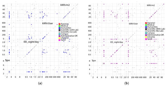
Figure 1.
Scatter plot matrix for the Unito’s buildings stock with respect to four attributes: type of building (1–9), the night/day energy efficiency index, the energy consumption per user and the energy consumption per square meter.
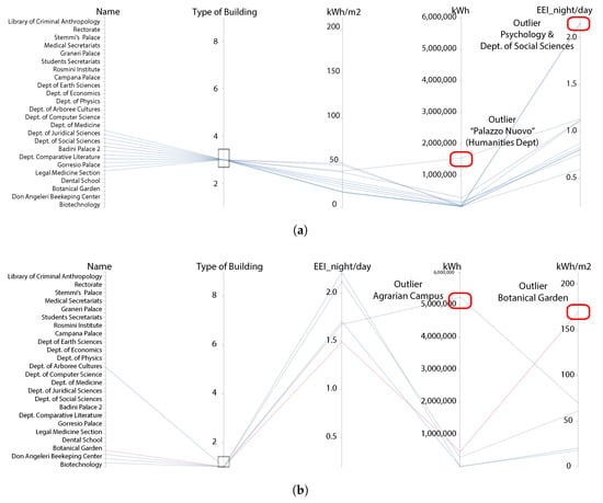
Figure 2.
Parallel coordinates method for the Unito’s buildings stock for two building functions—(a) Humanities Depts. and (b) Agrarian Depts.—with respect to four attributes: type of building (1–9), the night/day energy efficiency index, absolute annual energy consumption and the energy consumption per square meter.
The Scatter Plot Matrix is the generalization of the Scatter Plot, as described by Cottafava et al. [79], and is publicly available at https://goo.gl/o4nn4f. Figure 1 shows the whole building stock of the University of Turin and reports 16 different single Scatter Plots. Respectively, the x-axis and y-axis, starting from the bottom-left graph, report the following attributes: Type of building, the day/night energy efficiency index, the annual energy consumption per user and the annual energy consumption per meter square. The four graphs on the diagonal, as for a correlation matrix, has the same attribute on both x-axis and y-axis. Each cluster is identified with a different color and it can be highlighted simply selecting the type of the building in the bottom-left graph. The nine labeled colors are: red (Agrarian Depts.), green (Medical Depts.), blue (Humanities Depts.), black (Scientific Depts.—with lab.), grey (Scientific Depts.—without lab.), sky-blue (Large complexes), yellow (Libraries) and pink (Sport infrastructure). In particular, Figure 1a reports, as an example, the Humanities Departments and Figure 1b shows the Administrative Offices of the University of Turin. This visualization configuration allows checking if buildings with the same label lie on the same 1-D cluster, simply observing points distribution on the left and bottom plots. The tool here described is publicly available at https://goo.gl/ZJem9h. The Parallel Coordinates method also allows displaying various attributes for hundred points with a different visualization configuration. This approach permits a data miner to analyze dependent, or independent, attributes and to detect anomalies or precise trends and correlation among different attributes as in a pattern recognition problem. Figure 2 shows the entire Unito building stock with respect to four different attributes: the type of the building, the annual energy consumption per square meter, the absolute annual energy consumption and the day/night energy efficiency index. In this case, the nine clusters are labeled with number 1–9 and represented by the first vertical axis. Respectively, 1–9, the clusters correspond to the following: Agrarian Depts., Medical Depts., Humanities Depts., Scientific Depts.—with lab, Scientific Depts.—without lab, Large Complexes, Libraries and Sport Infrastructure. As for the Scatter Plot Matrix, in this case, the brush function allows a data miner, or a policy maker/energy manager, to highlight precise subset of the whole dataset. This feature permits to exploit the property Bumping the boundaries = to bound the clusters. Figure 2a,b, respectively, shows Humanities Depts. and Agrarian Depts. It is possible to notice quite precise fluxes/patterns of polygonal lines with a high density. The tool we used is publicly available at: https://goo.gl/4aHYuj.
4.1.3. Clustering Algorithm
The k-means algorithm has been used to identify and recognize clusters depending on three main attributes, annual absolute energy consumption, annual energy consumption per square meter and the day/night energy efficiency index, avoiding the energy consumption per user due to lack of data for administrative offices and other buildings. In this section, first, we report some considerations on the right number of clusters found thanks to the elbow method. We select the best configuration for each k—i.e., the lowest WSS—running 1000 MonteCarlo simulations. The elbow method suggests, as previously defined in data visualization analysis, that the right number of k is between 9 and 10, where the WSS slightly stops decreasing. Figure 3 shows the elbow plot with the WSS index on the y-axis and k, the number of clusters, on the x-axis. In Table 1, we report data obtained related to WSS, to the Davies–Bouldin index and to the silhouette index. Silhouette index is constant for different k while WSS and DB index decrease as k increases. Since silhouette index lies in , where a silhouette index of means a bad cluster correlation and 1 a good one, the obtained clusters represent a quite good configuration.
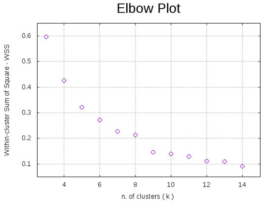
Figure 3.
Elbow method. The plot shows within-cluster sum of square vs. k ( of clusters). The right k number is between 9 and 10.

Table 1.
Best configuration evaluation index.
4.1.4. Comparison between DataViz and k-Means Clusters
Once the best number of clusters () was chosen, two external evaluation indices—the Rand index and the Fowlkes–Mallows index—were computed comparing clusters obtained by the k-means and the previously defined clusters within the Data Visualization Section. To obtain the best configuration, further 10,000 MonteCarlo simulations were run with the chosen maximizing the Rand index and choosing the respective cluster configuration. Table 2 reports the best cluster configuration result with respect to the Rand index.
Table 2.
Best external evaluation index.
4.2. Setting Thresholds
Starting from the Parallel Coordinates graph, we defined alert thresholds for the main six clusters, i.e., Scientific Depts. (without lab.), Scientific Depts. (with lab.), Humanities, Agrarian and Medical Depts. and Administrative Offices. Results and alert thresholds are reported in Table 3 with respect two main attributes and kWh/year∗m. We do not report absolute energy consumption per year because it is not interesting as a general index for energy efficiency. Table 3 shows that clusters corresponding to Scientific Depts. (with lab.), Agrarian and Medical Depts. have an high day/night energy efficiency index, as expected. Scientific Depts. (with lab.) shows a higher energy consumption per meter square with respect to Agrarian and Medical Depts. and in general with respect to all other clusters. Administrative Offices, Scientific Depts. (without lab.) and Humanities Depts., instead, have a common behavior with low kWh/year∗m and . Scientific Depts. (without lab), generally, present a slightly higher energy consumption at night.
Table 3.
Thresholds for consumption per square meter and for day/night energy efficiency index.
4.3. Monitoring Trends
The final step of the presented process is based on an application of the parallel coordinates method. In this case, we plot different annual energy consumptions on a different axis (each axis represents a different year) where only one attribute may be plotted. This tool, shown in Figure 4, allows visualizing the historical trend of a chosen energy efficiency index. A useful feature is the possibility to highlight simultaneously various buildings to observe their historical trends. By simply hoovering the mouse on each polyline, the building energy consumption for the chosen year is shown. By clicking on it, the polyline is highlighted, as shown in Figure 4, where “Library Dept. Philological Sciences” (violet) and the “Rectorate” (orange) stand out. The tool here described is publicly available at https://goo.gl/YuPTRB.
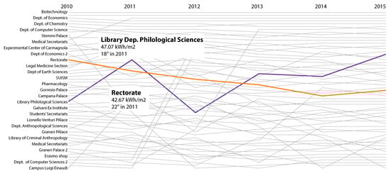
Figure 4.
Interactive data visualization tool to monitor historical trends based on the Parallel Coordinates method.
5. Discussion
The first aim of this paper is to determine a process to set general hypotheses on building clusters with respect to energy efficiency indices. A clusters hypothesis has been previously stated relying on the background knowledge of the energy management staff at the University of Turin. We envisage this step as a limit of this study, since it requires a preliminary effort by a human task force that is not always reliable, available, competent or even present. However, the time required in this phase is widely compensated by the easiness of the subsequent steps and the replicability of the monitoring phase in each institution able to offer at least the energy bill data source.
The clusters hypothesis has been made based on main building function and then it has been verified via two methodologies for the identification of buildings clusters: a data visualization approach and a clustering algorithm.
The data visualization approach allowed recognizing the validity of the clustering hypothesis. In fact, after labeling each building with a precise function, it is possible to match each building within a precise cluster straightforwardly (via the brush function). In this way, it is possible to immediately identify outliers and set rough alert thresholds, as described in Section 4.2 and in Table 3.
This method made us identify some outliers in the Unito case study. For instance, the Physics Dept. and the Biotechnology Dept. are two outliers within the cluster “Scientific Depts.—with laboratory”. High consumption per square meter and high day/night energy efficiency index are due both to large IT centres and to electric chillers running 24/24 h. Within the “Agrarian Depts.” cluster, the botanical garden is another outlier, with its very high consumption per square meter. The Agrarian Campus has been identified as an outlier, too, with respect to its annual energy consumption. Looking into that, one can infer that, since it hosts many thousands of students and very specific function related to field experiments and greenhouses maintenance, its energy behavior must be different and must be treated differently. Within the “Medical Depts.” cluster, the Dental School and the Legal Medicine Section are outliers compared to an average energy consumption or a day/night energy efficiency index. Again, a more detailed data source analysis reveals that the Dental School has a large electrical energy consumption due to the large amount of electrical technical machineries. As for the Legal Medicine Section, the reason of the high night consumption is the presencee and the mortuary rooms, asking for a constant air conditioning system, which is very costly especially during spring and summer seasons. Within the “Humanities Depts.” cluster, there are two outliers, the Social Science Dept. and the Psychology Dept., with respect to the day/night index: the reasons for this anomalous consumption is still under study at the Unito’s facility management office after a signaling coming from this work. “Palazzo Nuovo” (Humanities Dept) has one of the highest number of students and classrooms within the same building, thus explaining its higher energy request. Within the “Scientific Depts—without laboratory”, two outliers emerge: the Management Dept and Torino Exhibitions. The first one has a high consumption per square meter and a high annual consumption because the energy meter counts also the consumption of the Regional IT center, while “Torino Exhibitions” has a very high day/night index because of the secondary function of the building (art exhibitions, fairs and other types of events). Finally, the “Administrative offices” cluster has three outliers: Stemmi’s Palace, Tobacco Factory and Students’ secretariat. These three buildings have a high day/night index due to different reasons. The first one is the main building for the technical directions of the university and it hosts a lot of IT servers. Other reasons are under investigation. The other two buildings, instead, are two multifunctional buildings hosting public events for the City of Turin.
As a second step, a clustering algorithm has been used to test the initial hypothesis. The test was made exploiting two external indices—i.e., the Rand index and the Fowlkes–Mallows index—comparing the clusters configuration hypothesis (hp0) and the obtained clusters thanks to the k-means algorithm. The obtained clusters configuration with may be compared with the clusters hypothesis (Rand index = 0.769). k-means, due to its algorithm’s basic principles, similar to many other clustering algorithm, is strongly affected by local optimum and outliers. In fact, with a deeper analysis on clusters details, k-means algorithm is able to well-identify outliers—e.g., Management Dept., Biotechnology Dept. or Agrarian Campus—but it recognizes some clusters without physical explanation due to local optimum. For instance, the Department of Arboree Cultures (hp0: Agrarian Depts. cluster) and the Tobaccoes Factory (hp0: administrative offices cluster) or the Don Angeleri Beekeeping Center (Agrarian Depts. cluster) and the Psychology Dept. (hp0: Humanities Depts. cluster) always lie within the same cluster without any other point because they have a very common energy consumption behavior. The three clusters hp0: Administrative Offices, Humanities Depts. and Scientific Depts. (without laboratories) are mixed together in only two clusters. Scientific Depts. (with laboratories) cluster is well-recognized losing one of the outliers described in data visualization approach, the Biotechnology Dept., and gaining two outliers from other clusters, the Botanical Garden and the Dental School. Many outliers, identified in the DataViz approach, are aggregated into the same cluster—e.g., Tobaccoes Factory, Torino Exhibitions, Legal Medicine Section, Social Science Dept and Students’ secretariat. This behavior reveals that a possible new cluster hypothesis should include a multifunctional building cluster. Finally, the two main campuses Campus Luigi Einaudi and the Agrarian Campus are always grouped together, representing a reasonable choice. The Management Dept., outlier within the Scientific Depts. (without lab) cluster, and the Biotechnology Dept. are clustered alone. In conclusion, k-means clustering algorithm recognizes very accurately the main clusters—identified as campuses, service industry buildings and Scientific Depts.—confirming our initial hypothesis but is not able, as expected, to recognize slight differences between Humanities Depts., Scientific Buildings (without lab) and Administrative Offices.
6. Conclusions
To conclude, this data visualization approach offers a simple way to identify outliers and to set alerts energy consumption thresholds for each buildings function, but the reasons for the inefficiency have to be explained with deeper analyses. For instance, with the help of specific mapping tools (e.g., GIS) to localise buildings and visualize their location within the city or with the support of the facility management, further features and informations, that did not emerge during the preliminary labelling phase, may be revealed. As a methodological caveat, this approach reveals outliers within clusters defined ex-ante; therefore, every multifunctional cluster is shown as an outlier of its own cluster, and that can be a limit if a cluster is the result of a preliminary wrong human inference. However, DataViz techniques revealed to be very useful to explore quickly and simply a large building stock, identifying the least efficient buildings and clustering buildings according to their functions. Moreover, the results are presented in a user-friendly graphical interface, understandable and accessible to facility managers, even if they are not expert in energy monitoring. This improves the decision process, supporting the diagnosis of energy faults and therefore prioritizing alternatives and energy-efficient strategies, achieving faster energy saving. The implementation of easy energy diagnostics tools and underlying analysis algorithms can lead to a systematic identification of more efficient operations. Last but not least, such clusterization can be used to group relatively similar buildings for comparison inside the university realm, thus providing precious and still lacking national/international thresholds for setting limits for energy consumptions. Similarly, since benchmarking policies require an accurate measurement of buildings relative to one another, this easy way of energy monitoring can act as a kick-off for a quick assessment of universities as an independent building/district class, and then tailor appropriate energy policies for it.
Our results revealed that clustering algorithms—k-means in our case—cannot be exploited to design useful clusters based on the function of the building, except for some macro—cluster like tertiary service buildings or campuses and scientific buildings. Moreover, the results show how the most interesting part of information in energy efficiency analysis is lost. In fact, data analysts or energy managers are usually interested in inefficient buildings, thus in outliers with respect to their cluster, even when clustering algorithms tend to aggregate outliers in the wrong cluster. This makes a humanized process always necessary and irreplaceable. At the city level, such data driven tools require a large penetration of metering systems and the possibility to use the private data of the entire building stock; these conditions are still not commonly met, but combined techniques need to be taken into account for future researches to achieve the desired level of granularity in the data source. Of course, identifying and removing causes of abnormal energy use ensures a more efficient environment and not just in terms of the building energy costs.
The algorithms we have applied appear computationally efficient and robust, and can be easily integrated into existing university campus building energy management and warning systems. Of course, further work is needed: (i) to build on this clustering technique; (ii) to provide additional datasets for training the algorithm; (iii) to adopt language processing tools for the automated reading of metered building/energy bills data.
Author Contributions
D.C. was the principal investigator. G.S. contributed in finding proper energy efficiency indices and A.T., Energy Manager of the University of Turin, helped to verify the results and to identify proper explanations for the outliers. P.G. supervised the work.
Acknowledgments
Support by the Fondazione Goria, program “Talenti per la Società Civile”, is gratefully acknowledged.
Conflicts of Interest
The authors declare no conflict of interest.
Nomenclature
List of Abbreviations
| GHG | Greenhouse Gas |
| HVAC | Heating, ventilating and conditiong |
| TRNSYS | Transient System Simulation Tool |
| EEI | Energy Efficiency Index |
| DataViz | Data Visualization |
| TOE | Tonne of oil equivalent |
| kWh | Kilowatt hour |
| WSS | Within-Cluster Sum of Square |
| Multidimensional Dataset | |
| n | Number of elements in dataset X |
| m | Number of attributes/dimensions of dataset X |
| Observation i of dataset X | |
| Real value of attribute j of observation i | |
| Observation subscript | |
| Minkowski (or Mahalanobis) distance between observation i and l | |
| p | Minkowski order |
| Jaccard Distance | |
| Within-Cluster Sum of Square | |
| Davies-Bouldin Index | |
| S | Silhouette Index |
| k | Number of Clusters |
| Observation i lying in cluster j | |
| The centroid of the cluster x | |
| Mean distance between any data in cluster x and the centroid of the cluster | |
| Number of points in cluster | |
| distance between points and | |
| Alert thresholds for attribute j | |
| Annual night/day Electrical Energy Efficiency Index | |
| Electrical energy consumption during working day for month i | |
| Electrical energy consumption during night and weekend for month i |
References
- Powell, J.B. Green Building Services. J. Int. Commer. Econ. 2015. [Google Scholar]
- Wilkinson, P.; Smith, K.; Beevers, S.; Tonne, C.; Oreszczyn, T. Energy, energy efficiency, and the built environment. Lancet 2007, 370, 1175–1187. [Google Scholar] [CrossRef]
- Newman, P. The environmental impact of cities. Environ. Urban. 2006, 18, 275–295. [Google Scholar] [CrossRef]
- Staff, I.E.A. Transition to Sustainable Buildings: Strategies and Opportunities To 2050; Organization for Economic Cooperation and Development: Paris, France, 2013. [Google Scholar]
- Lombardi, P.; Trossero, E. Beyond energy efficiency in evaluating sustainable development in planning and the built environment. Int. J. Sustain. Build. Technol. Urban Dev. 2013, 4, 274–282. [Google Scholar] [CrossRef]
- Brandon, P.S.; Lombardi, P.; Shen, G.Q. Future Challenges in Evaluating and Managing Sustainable Development in the Built Environment; John Wiley & Sons: Southern Gate, Chichester, UK, 2017. [Google Scholar]
- Ascione, F.; Bianco, N.; Stasio, C.D.; Mauro, G.M.; Vanoli, G.P. Addressing Large-Scale Energy Retrofit of a Building Stock via Representative Building Samples: Public and Private Perspectives. Sustainability 2017, 9, 940. [Google Scholar] [CrossRef]
- Giuseppina, C.; Galatioto, A.; Ricciu, R. Energy and economic analysis and feasibility of retrofit actions in Italian residential historical buildings. Energy Build. 2016, 128, 649–659. [Google Scholar]
- Bakar, N.N.A.; Hassan, M.Y.; Abdullah, H.; Rahman, H.A.; Abdullah, M.P.; Hussin, F.; Bandi, M. Sustainable energy management practices and its effect on EEI: A study on university buildings. In Proceedings of the Global Engineering, Science and Technology Conference, Dubai, UAE, 1–2 April 2013. [Google Scholar]
- Moghimi, S.F.A.; Mat, S.; Lim, C.; Salleh, E.; Sopian, K. Building energy index and end-use energy analysis in large-scale hospitals case study in Malaysia. Energy Effic. 2014, 7, 243–256. [Google Scholar] [CrossRef]
- González, A.B.R.; Díaz, J.J.V.; Caamano, A.J.; Wilby, M.R. Towards a universal energy efficiency index for buildings. Energy Build. 2011, 43, 980–987. [Google Scholar] [CrossRef]
- Ballarini, I.; Corgnati, S.P.; Corrado, V. Use of reference buildings to assess the energy saving potentials of the residential building stock: The experience of TABULA project. Energy Policy 2014, 68, 273–284. [Google Scholar] [CrossRef]
- Andaloro, A.P.; Salomone, R.; Ioppolo, G.; Andaloro, L. Energy certification of buildings: A comparative analysis of progress towards implementation in European countries. Energy Policy 2010, 38, 5840–5866. [Google Scholar] [CrossRef]
- Galatioto, A.; Ciulla, G.; Ricciu, R. An overview of energy retrofit actions feasibility on Italian historical buildings. Energy 2017, 137, 991–1000. [Google Scholar] [CrossRef]
- Ciulla, G.; Lo Brano, V.; D’Amico, A. Modelling relationship among energy demand, climate and office building features: A cluster analysis at European level. Appl. Energy 2016, 183, 1021–1034. [Google Scholar] [CrossRef]
- Yun, G.; Steemers, K. Behavioural, physical and socio economic factors in household cooling energy consumption. Appl. Energy 2011, 88, 2191–2200. [Google Scholar] [CrossRef]
- Wu, L.-M.; Chen, B.-S. Modeling of energy efficiency indicator for semi-conductor industry. In Proceedings of the IEEE International Conference on Industrial Engineering and Engineering Management, Singapore, 2–4 December 2007; IEEE: Piscataway, NJ, USA, 2007. [Google Scholar]
- Ferrer-Balas, D.; Lozano, R.; Huisingh, D.; Buckland, H.; Ysern, P.; Zilahy, G. Going beyond the rhetoric: System-wide changes in universities for sustainable societies. J. Clean. Prod. 2010, 18, 607–610. [Google Scholar] [CrossRef]
- Agdas, D.; Srinivasan, R.; Frost, K.; Masters, F. Energy Use Assessment of Educational Buildings: Toward a Campus-wide Sustainable Energy Policy. Sustain. Cities Soc. 2015, 17, 15–21. [Google Scholar] [CrossRef]
- Chung, M.; Rhee, E. Potential opportunities for energy conservation in existing buildings on university campus: A field survey in Korea. Energy Build. 2014, 78, 176–182. [Google Scholar] [CrossRef]
- Escobedo, A.; Briceño, S.; Juárez, H.; Castillo, D.; Imaz, M.; Sheinbaum, C. Energy consumption and GHG emission scenarios of a university campus in Mexico. Energy Sustain. Dev. 2014, 18, 49–57. [Google Scholar] [CrossRef]
- Evans, J.; Jones, R.; Karvonen, A.; Millard, L.; Wendler, J. Living labs and co-production: University campuses as platforms for sustainability science. Curr. Opin. Environ. Sustain. 2015, 16, 1–6. [Google Scholar] [CrossRef]
- Robinson, O.; Kemp, S.; Williams, I. Carbon management at universities: A reality check. J. Clean. Prod. 2014, 106, 109–118. [Google Scholar] [CrossRef]
- Del Mar Alonso-Almeida, M.; Marimon, F.; Casani, F.; Rodriguez-Pomeda, J. Diffusion of sustainability reporting in universities: Current situation and future perspectives. J. Clean. Prod. 2015, 106, 144–154. [Google Scholar] [CrossRef]
- Lauder, A.; Sari, R.F.; Suwartha, N.; Tjahjono, G. Critical review of a global campus sustainability ranking: GreenMetric. J. Clean. Prod. 2015, 108, 852–863. [Google Scholar] [CrossRef]
- NBS. China Statistical Yearbook; Technical Report; China Statistics Press: Beijing, China, 2012. [Google Scholar]
- Shriberg, M. Institutional assessment tools for sustainability in higher education: Strengths, weaknesses, and implications for practice and theory. Int. J. Sustain. High. Educ. 2002, 3, 254–270. [Google Scholar] [CrossRef]
- Haas, R. Energy efficiency indicators in the residential sector: What do we know and what has to be ensured? Energy Policy 1997, 25, 789–802. [Google Scholar] [CrossRef]
- Jollands, N.; Patterson, M. Four theoretical issues and a funeral: Improving the policy-guiding value of eco-efficiency indicators. Int. J. Environ. Sustain. Dev. 2004, 3, 235–261. [Google Scholar] [CrossRef]
- Sonetti, G.; Lombardi, P.; Chelleri, L. True Green and Sustainable University Campuses? Toward a Clusters Approach. Sustainability 2016, 8. [Google Scholar] [CrossRef]
- Yik, F.; Burnett, J.; Prescott, I. Predicting air-conditioning energy consumption of a group of buildings using different heat rejection methods. Energy Build. 2001, 33, 151–166. [Google Scholar] [CrossRef]
- Howard, B.; Parshall, L.; Thompson, J.; Hammer, S.; Dickinson, J.; Modi, V. Spatial distribution of urban building energy consumption by end use. Energy Build. 2012, 45, 141–151. [Google Scholar] [CrossRef]
- Yang, C.; Létourneau, S.; Guo, H. Developing Data-driven Models to Predict BEMS Energy Consumption for Demand Response Systems. In Modern Advances in Applied Intelligence; Ali, M., Pan, J.S., Chen, S.M., Horng, M.F., Eds.; Springer International Publishing: Cham, Switzerland, 2014; pp. 188–197. [Google Scholar]
- Hong, T.; Yang, L.; Hill, D.; Feng, W. Data and analytics to inform energy retrofit of high performance buildings. Appl. Energy 2014, 126, 90–106. [Google Scholar] [CrossRef]
- Yalcintas, M. An energy benchmarking model based on artificial neural network method with a case example for tropical climates. Int. J. Energy Res. 2006, 30, 1158–1174. [Google Scholar] [CrossRef]
- Yalcintas, M.; Ozturk, U.A. An energy benchmarking model based on artificial neural network method utilizing US Commercial Buildings Energy Consumption Survey (CBECS) database. Int. J. Energy Res. 2007, 31, 412–421. [Google Scholar] [CrossRef]
- Fan, C.; Xiao, F.; Wang, S. Development of prediction models for next-day building energy consumption and peak power demand using data mining techniques. Appl. Energy 2014, 127, 1–10. [Google Scholar] [CrossRef]
- Inselberg, A. Multidimensional Detective. In Proceedings of the IEEE Symposium on Information Visualization, Phoenix, AZ, USA, 20–21 October 1997. [Google Scholar]
- Card, S.K.; Mackinlay, J.; Shneiderman, B. Readings in Information Visualization: Using Vision to Think; Morgan Kaufman: San Francisco, CA, USA, 1999. [Google Scholar]
- NIST-SEMATECH. E-Handbook of Statistical Methods; NIST: Gaithersburg, MD, USA, 1997.
- Bostock, M.; Ogievetsky, V.; Heer, J. D3: Data-Driven Documents. IEEE Trans. Vis. Comput. Graph. 2011, 12, 2301–2309. [Google Scholar] [CrossRef] [PubMed]
- Bezanson, J.; Edelman, A.; Karpinski, S.; Shah, V.B. Julia: A fresh approach to numerical computing. arXiv, 2014; arXiv:1411.1607. [Google Scholar]
- Keim, D. Visual Techniques for Exploring Databases; Technical Report; NIST: Gaithersburg, MD, USA, 2003. [Google Scholar]
- Inselberg, A. The plane with parallel coordinates. Vis. Comput. 1985, 1, 69–97. [Google Scholar] [CrossRef]
- Feiner, S.; Beshers, C. Worlds within worlds: Metaphors for exploring n-dimensional virtual worlds. In Proceedings of the 3rd Annual ACM SIGGRAPH Symposium on User Interface Software and Technology, Snowbird, UT, USA, 3–5 October 1990; pp. 76–83. [Google Scholar]
- Cleveland, W. Visualizing Data; Hobart Press: Summit, NJ, USA, 1993. [Google Scholar]
- Borg, I.; Groenen, P.J.F. Modern Multidimensional scaling: Theory and Applications. Vis. Comput. 2005, 2, 276–278. [Google Scholar] [CrossRef]
- Keller, P.R.; Keller, M.M. Visual Cues-Practical Data Visualization. IBM Syst. J. 1993, 33. [Google Scholar] [CrossRef]
- Ariaudo, F.; Balsamelli, L.; Corgnati, S.P. Il Catasto Energetico dei Consumi come strumento di analisi e programmazione degli interventi per il miglioramento dell’efficienza energetica di ampi patrimoni edilizi. In Proceedings of the 48th International Conference AICARR, Baveno, VCO, Italy, 22–23 September 2011; pp. 547–559. [Google Scholar]
- Cottafava, D.; Gambino, P.; Baricco, M.; Tartaglino, A. Multidimensional analysis tools for energy efficiency in large building stocks. In Proceedings of the 12th Conference on Sustainable Development of Energy, Water and Environment Systems, Dubrovnik, Croatia, 4–8 October 2017. [Google Scholar]
- Jain, A.; Dubes, R. Algorithms for Clustering Data; Prentice-Hall: Upper Saddle River, NJ, USA, 1988. [Google Scholar]
- Xu, R.; Wunsch, D. Survey of clustering algorithms. IEEE Trans. Neural Netw. 2005, 16, 645–678. [Google Scholar] [CrossRef] [PubMed]
- Xu, D.; Tian, Y. A Comprehensive Survey of Clustering Algorithms. Ann. Data Sci. 2015, 2, 165–193. [Google Scholar] [CrossRef]
- Kassambara, A. Practical Guide To Cluster Analysis in R; CreateSpace: North Charleston, SC, USA, 2017. [Google Scholar]
- Maulik, U.; Bandyopadhyay, S. Performance evaluation of some clustering algorithms and validity indices. IEEE Trans. Pattern Anal. Mach. Intell. 2002, 24, 1650–1654. [Google Scholar] [CrossRef]
- Starczewski, A.; Krzyżak, A. Performance Evaluation of the Silhouette Index. In Artificial Intelligence and Soft Computing; Rutkowski, L., Korytkowski, M., Scherer, R., Tadeusiewicz, R., Zadeh, L.A., Zurada, J.M., Eds.; Springer International Publishing: Cham, Switzerland, 2015; pp. 49–58. [Google Scholar]
- Rand, W.M. Objective Criteria for the Evaluation of Clustering Methods. J. Am. Stat. Assoc. 1971, 66, 846–850. [Google Scholar] [CrossRef]
- Kosub, S. A note on the triangle inequality for the Jaccard distance. arXiv, 2016; arXiv:1612.02696. [Google Scholar]
- Fowlkes, E.B.; Mallows, C.L. A Method for Comparing Two Hierarchical Clusterings. J. Am. Stat. Assoc. 1983, 78, 553–569. [Google Scholar] [CrossRef]
- Nagpal, A.; Jatain, A.; Gaur, D. Review based on data clustering algorithms. In Proceedings of the 2013 IEEE Conference on Information Communication Technologies, Thuckalay, Tamil Nadu, India, 11–12 April 2013; pp. 298–303. [Google Scholar]
- Ahmad, A.; Dey, L. A K-mean Clustering Algorithm for Mixed Numeric and Categorical Data. Data Knowl. Eng. 2007, 63, 503–527. [Google Scholar] [CrossRef]
- Macqueen, J. Some methods for classification and analysis of multivariate observations. In Proceedings of the 5-th Berkeley Symposium on Mathematical Statistics and Probability, Berkeley, CA, USA, 21 June–18 July 1967; pp. 281–297. [Google Scholar]
- Park, H.; Jun, C. A simple and fast algorithm for K-medoids clustering. Expert Syst. Appl. 2009, 36, 3336–3341. [Google Scholar] [CrossRef]
- Kaufman, L.; Rousseeuw, P. Partitioning around Medoids (Program Pam); Wiley: Hoboken, NJ, USA, 1990; pp. 126–160. [Google Scholar]
- Ng, R.T.; Jiawei, H. CLARANS: A method for clustering objects for spatial data mining. IEEE Trans. Knowl. Data Eng. 2002, 14, 1003–1016. [Google Scholar] [CrossRef]
- Kaufman, L.; Rousseeuw, P. Partitioning around Medoids (Program Pam); Wiley: Hoboken, NJ, USA, 1990; pp. 68–120. [Google Scholar]
- Guha, S.; Rastogi, R.; Shim, K. CURE: An Efficient Clustering Algorithm for Large Data sets. In Proceedings of the ACM SIGMOD Conference, Seattle, WA, USA, 2–4 June 1998. [Google Scholar]
- Zhang, T.; Ramakrishnan, R.; Livny, M. BIRCH: An efficient data clustering method for very large databases. In Proceedings of the ACM SIGMOD International Conference on Management of Data (SIGMOD), Montreal, QC, Canada, 4–6 June 1996; pp. 103–114. [Google Scholar]
- Karypis, G.; Han, E.H.; Kumar, V. Chameleon: Hierarchical clustering using dynamic modeling. Computer 1999, 32, 68–75. [Google Scholar] [CrossRef]
- Ketchen, J.D.; Shook, C.L. The application of cluster analysis in strategic management reasearch: An analysis and critique. Strateg. Manag. J. 1996, 17, 441–458. [Google Scholar] [CrossRef]
- Thorndike, R.L. Who belongs in the family? Psychometrika 1953, 18, 267–276. [Google Scholar] [CrossRef]
- Pollard, K.S.; Van Der Laan, M.J. A method to identify significant clusters in gene expression data. In Proceedings of the SCI (World Multiconference on Systemics, Cybernetics and Informatics), Orlando, FL, USA, 14–18 July 2002; Volume 2, pp. 318–325. [Google Scholar]
- Tibshirani, R.; Walther, G.; Hastie, T. Estimating the number of clusters in a data set via the gap statistic. J. R. Stat. Soc. Ser. B (Stat. Methodol.) 2001, 63, 411–423. [Google Scholar] [CrossRef]
- Sheikholeslami, G.; Chatterjee, S.; Zhang, A. Wavecluster: A Multi-Resolution Clustering Approach for Very Large Spatial Databases. VLDB 1998, 98, 428–439. [Google Scholar]
- Smyth, P. Clustering Using Monte Carlo Cross-Validation. In Proceedings of the Second International Conference on Knowledge Discovery and Data Mining, KDD’96, Portland, Oregon, 2–4 August 1996; Volume 1, pp. 26–133. [Google Scholar]
- Monti, S.; Tamayo, P.; Mesirov, J.; Golub, T. Consensus clustering: A resampling-based method for class discovery and visualization of gene expression microarray data. Mach. Learn. 2003, 52, 91–118. [Google Scholar] [CrossRef]
- Roth, V.; Lange, T.; Braun, M.; Buhmann, J. A resampling approach to cluster validation. In Compstat; Springer: Heidelberg, Germany, 2002; pp. 123–128. [Google Scholar]
- Wang, J. Consistent selection of the number of clusters via crossvalidation. Biometrika 2010, 97, 893–904. [Google Scholar] [CrossRef]
- Cottafava, D.; Gambino, P.; Baricco, M.; Tartaglino, A. Energy efficiency in a large university: The UniTo experience. In Proceedings of the Sustainable Built Environment. Towards Post Carbon Cities, Turin, Italy, 18–19 February 2016; pp. 92–101. [Google Scholar]
© 2018 by the authors. Licensee MDPI, Basel, Switzerland. This article is an open access article distributed under the terms and conditions of the Creative Commons Attribution (CC BY) license (http://creativecommons.org/licenses/by/4.0/).