Residential Electricity Consumption Level Impact Factor Analysis Based on Wrapper Feature Selection and Multinomial Logistic Regression

Abstract

This paper aims to identity the significant impact factors (IFs) of the residential electricity consumption level (RECL) and to better understand the influence mechanism of IFs on RECL. The analysis of influence mechanism is commonly through regression model where feature selection must first be performed to pick out non-redundant IFs that is highly correlated with RECL. In contrast to the existing studies, this study recognizes the problem that majority feature selection methods (e.g., step regression) are limited to the identification of linear relationships and proposes a novel wrapper feature selection (WFS) method to address this issue. The WFS is based on genetic algorithm (GA) and multinomial logistic regression (MLR). GA is a searching algorithm used to generate different feature subsets (FSs) that consist of several IFs. MLR is a modeling algorithm used to score these FSs. Further, maximal information coefficient (MIC) is utilized to verify the validity of WFS for selecting IFs. Finally, MLR based explanatory model is established to excavate the relationship between selected IFs and RECL. The results of Ireland dataset based case study show that WFS can identify the significant and non-redundant IFs that are linearly or nonlinearly related to RECL. The details about how selected IFs affect RECL are also provided via the explanatory model. Such research can provide useful guidance for a wide range of stakeholders including local governments, electric power companies, and individual households.

1. Introduction

1.1. Background and Motivation

The electricity consumption in the residential sector has experienced a substantial increase over the past 40 years [1,2]. The world total electricity consumption reached 20,200 TWh in 2015, increased by 1.6% annually [3]. It was reported by the International Energy Agency (IEA) that the share of total electricity consumption in the residential sector has increased from approximately 24.2% in 1974 to 31.1% in 2015 [3]. In addition, the majority of the electricity is still generated by thermal power plant accompanied by greenhouse gas (GHG) emissions [4], thus residential dwellings also have a certain responsibility for the GHG emissions that result in global warming [5]. Therefore, considering the environmental requirements established by the climate change agreements [6,7], targeted measures for the reduction of electricity consumption should be implemented by relevant departments. This is helpful for the enhancement of energy efficiency and the promotion of environmental sustainability initiatives [8].

The residential electricity consumption level (RECL) is influenced by various characteristics of dwelling, appliance, occupants and their attitudes [9,10]. The design of effective electricity conservation scheme relies on the comprehensive understanding of main factors that affect the RECL. How to figure out these important impact factors (IFs) and reveal the complex relationship between IFs and RECL is an essential problem for improving energy efficiency. Such IF analysis of RECL is useful for a wide range of stakeholders, providing a valid guidance for local governments to develop electricity conservation policies, electric power companies to design tailor-made DR programs [11,12], system operators to address the challenge (caused by the uncertainty of load demand) in the security-constrained unit commitment program [13], and individual households to reduce the expense of electricity [14,15].

1.2. Literature Review

Over the past decade, a growing research trend is related to the evolution of environmental awareness, mainly including five hot topics [8]: (1) factors influencing energy efficiency and environmental sustainability initiatives; (2) classification of energy efficiency and environmental sustainability initiatives; (3) impact of energy efficiency and environmental sustainability on supply chain performance; (4) customer perspective in energy-efficient and sustainable supply chain; (5) Information and communication technologies (ICTs) supporting energy efficiency and environmental sustainability initiatives. As for a newly emerging topic, IF analysis of RECL has recently become the considerable focus of current electrical research field. This topic is close to the above mentioned two topics, namely factors influencing energy efficiency and customer perspective in energy-efficient. Specifically, IF analysis of RECL is kind of research work, aiming to provide a rational guidance for the enhancement of the energy efficiency from the customer perspective.

According the previous related literatures, regression models are commonly employed method that is applied to understand the specific influence mechanism between IFs and RECL. Nevertheless, high dimensionality and multiple correlations of IFs will worsen model reliability and result in wrong IF analysis of RECL. Thus, feature selection that aims to select significant and non-redundant IFs is regarded as an essential step before model establishment [16]. In machine learning, feature selection refers to the process of selecting a subset of relevant features (i.e., IFs) during the model establishment in order to maximally preserve the features of original consumption data. Generally, feature selection methods can be classified into three categories: (1) filter method (2) wrapper method (3) embedded method.

For filter methods, features are ranked according to correlation coefficients such as the Pearson coefficient. All the features with correlation coefficients larger than a given threshold are then selected [17]. A Chinese example used bivariate correlation and path analysis to identify linear relationships between factors and electricity consumption [18]. p-value test is a common method to judge the significance of factors. It is used to remove the factors with the value of parameter α smaller than 0.05 [1,19]. Similarly, the Australian study conducted by Fan et al. [20] put all the factors into a general regression model. The factors that did not pass a 95% confidence interval significance level test were removed one by one until the remained factors meet the p-value test. Filter methods are simple with low computational complexity, but it is difficult to set a suitable threshold and identify the redundancy among factors.

Unlike filter methods, wrapper methods can not only take the performance of established model into consideration, but also delete redundant factors. Wrapper methods are the combination of search algorithm and modeling algorithm, where the former is used to generate new feature subsets (FSs) and the latter is used to score these different FSs. The prevalent wrapper method in current research is stepwise regression, which incorporates factors one by one and simultaneously removes insignificant or redundant factors to better fit the final linear regression model with higher adjusted R² [21,22]. In a word, wrapper methods with higher computation complexity outperform filter methods in the following two aspects: (1) the correlation between candidate feature and other features is considered at the modelling stage; (2) the model is optimized to successfully eliminate irrelevant and redundant features, as well as improve the precision of the model.

Embedded methods perform feature selection and model establishment simultaneously via a specific algorithm that takes advantage of its own feature selection process [23]. One example in residential electricity analysis is the LASSO method applied by Huebner et al. in [9]. This method is used to establish a linear model, which can shrink regression coefficients of non-relevant and redundant factors to zero based on a penalty parameter. Features with non-zero regression coefficients are “selected”. Embedded methods are more efficient than other two feature selection methods through incorporating feature selection as part of the model establishment. But the reasonable value of key parameters (e.g., the penalty parameter L1 in LASSO algorithm) is difficult to set. Furthermore, the model established by such algorithm is not always what researchers needed in later analysis. This means that the optimal FS selected by embedded methods is not certainly able to best optimize the performance of newly established regression model.

Given the merits and drawbacks of aforementioned feature selection methods, especially that most feature selection methods of previous literature are merely able to identify linear relationships, a thorough consideration is needed to decide which method is more applicable in actual research.

1.3. Contributions

This paper aims to identify significant IFs of RECL and understand how these IFs affect RECL. According to previous literature, residential electricity consumption is driven by numerous factors, but their analysis results always vary across different studies [9,10]. Besides factors studied in previous research, new factors are taken into consideration in this study, and they can be classified into four categories: (1) dwelling characteristics (2) socio-demographics (3) appliances and cooking-heating methods (4) energy-saving attitudes.

To establish a reliable regression model and fill the gap mentioned in Section 1.2, wrapper feature selection (WFS) is proposed in this paper, which combines genetic algorithm (GA) with multinomial logistic regression (MLR). GA is a searching algorithm used to generate new FSs that consist of one or more IFs. And MLR is a modeling algorithm used to score these FSs. Further, as a new measure of the association between two variables, maximal information coefficient (MIC) is used to verify the validity of WFS for selecting IFs. The MICs between selected IFs and RECL are calculated to figure out whether these IFs have significant effects on RECL. Meanwhile, the MICs between removed IFs and selected IFs are also calculated to verify the multiple correlations among them. Finally, MLR based explanatory model is established to explain the effects of selected IFs on RECL. The main contributions of this paper can be summarized as follows. First, a new feature selection method named WFS is proposed to identify significant and non-redundant IFs that are linearly or non-linearly related to RECL. Second, a massive set of data with various types of IFs is newly investigated to provide a systematical analysis on the impact of IFs on RECL in more comprehensive and in-depth perspectives via MLR.

The rest of the paper is organized as follows: Section 2 gives a description of datasets used in this paper. Section 3 briefly introduces WFS, MIC and MLR. In Section 4, the assessment of the validity of WFS for selecting IFs is presented, as well as the illustration of influence mechanism between IFs and RECL. The application of this study is proposed in Section 5. At the end, Section 6 highlights the concluding remarks and future work directions.

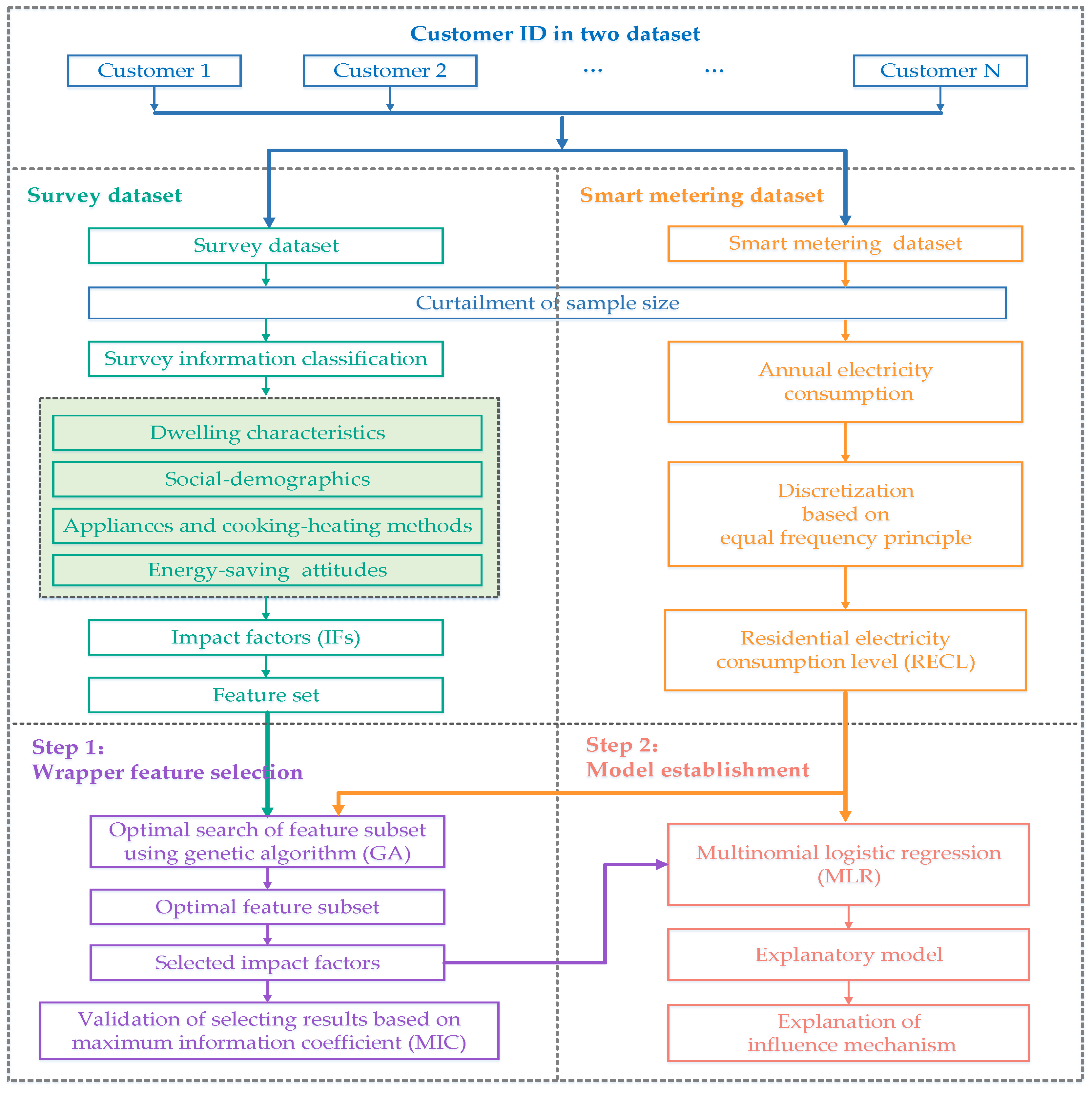
2. Description and Processing of Dataset

The Smart Metering Electricity Customer Behavior Trials (CBTs) were carried out during 2009 and 2010 by Commission for Energy Regulation (CER) in Ireland [24]. The overall objective of the trial was to test the impact and viability of smart metering technology in Ireland, and to explore the electricity demand reducing effects of various feedback mechanisms and time-of-use tariffs. Over 4000 Irish residential customers participated in the trials with an electricity smart meter installed in their homes and agreed to finish a comprehensive survey concerning residential characteristics, such as social demographics, appliance ownership and energy-saving altitudes. This research makes a full use of the data collected by CER to figure out the relationship between residential characteristics and electricity consumption.

2.1. Smart Metering and Survey Dataset

The smart metering dataset is comprised of the daily electricity consumption data of 4232 residential customers at 30 min interval over one and a half year. We selected the data of a full year from 1st January to 31st December 2010 for this research and the dataset is reduced to 3401 customers after removing 831 customers with missing data. The annual electricity consumption based classification result of customers is considered as the response variable in the explanatory model, which is further described in Section 2.2.

As a part of the CBTs, the survey is designed to collect the information about the various characteristics of dwelling, occupants, appliance and energy-saving attitudes. Every record of each customer in the surveys dataset is linked to the corresponding records in the smart metering dataset through the unique ID of each customer. Among these 3401 customers, we were able to identify 3311 valid surveys by the ID. Hence, the sample size was finally trimmed to 3311 customers for the further analysis in this paper. Furthermore, the residential characteristics (i.e., IFs) presented in

Table 1. Overview of residential characteristics in survey dataset.

Residential Characteristics(i.e., IFs)	Proportion of Each Answer (%)
Category1: Dwelling characteristics
Dwelling type	Apartment(1.7) | Semi-detached(30.1) | Detached(27.2) | Terraced(14.1) |Bungalow(27.0)
Dwelling age	0–20 years(34.2) | 20–40 years(32.9) | 40 years +(32.9)
No. a of bedrooms	1(1.1) | 2(8.1) | 3(43.8) | 4(35.3) | 5+(11.7)
POESL b	0(21.5) | 5%(26.4) | 50%(16.8) | 75%(16.8) | 100%(18.5)
PODGW c	0(7.9) | 25%(1.9) | 50%(2.8) | 75%(2.7) | 100%(84.6)
Insulated external walls	Yes(57.6) | no(30.9) | don’t know(11.4)
Category2: Socio-demographics
Sex of householder	Female(50.6) | Male(49.4)
Age of householder	18–45 years(30.2) | 46–65 years(46.4) | 65 years+(23.4)
Employment status of CIE d	Employee(47.0) | Self-employed(12.6) | Unemployed(8.5) | Retired or keeper(32.0)
Education level of CIE	No formal education(1.3) | Primary(11.2) | Second level(45.5) | Third level(36.6) |Refused(5.3)
Living form	Live alone(19.1) | All people are adults(52.8) | With adults and children(28.0)
No. of people under 15 years old	0(72.0) | 1(12.0) | 2(9.7) | 3(4.6) | 4+(1.7)
Category3: Appliance and cooking -heating methods
Appliances ownership
No. of washing machine	0(1.7) | 1(97.6) | 2(0.7) | 2+(0)
No. of tumble dryer	0(31.3) | 1(68.5) | 2(0.2) | 2+(0)
No. of dishwasher	0(33.5) | 1(66.2) | 2(0.3) | 2+(0)
No. of electric shower (instant)	0(30.8) | 1(63.2) | 2(5.5) | 2+(0.5)
No. of electric shower (pumped)	0(70.9) | 1(26.4) | 2(2.2) | 2+(0.5)
No. of electric cooker	0(22.9) | 1(76.7) | 2(0.3) | 2+(0.1)
No. of electric heater	0(69.2) | 1(23.7) | 2(5.3) | 2+(1.8)
No. of refrigerator	0(49.6) | 1(48.5) | 2(1.8) | 2+(0.1)
No. of water pump	0(80.5) | 1(19.0) | 2(0.5) | 2+(0)
No. of immersion	0(23.2) | 1(76.2) | 2(0.4) | 2+(0)
No. of TV < 21 inch	0(35.3) | 1(39.0) | 2(18.1) | 3(5.6) | 3+(2.0)
No. of TV > 21 inch	0(15.5) | 1(50.8) | 2(25.4) | 3(6.0) | 3+(2.3)
No. of desk-top computers	0(52.1) | 1(45.0) | 2(2.4) | 3(0.3) | 3+(0.2)
No. of laptop computers	0(46.3) | 1(42.1) | 2(8.5) | 3(2.1) | 3+(1.0)
No. of games consoles	0(66.5) | 1(22.6) | 2(8.1) | 3(2.1) | 3+(0.7)
Appliances usage(AU)
Washing machine	Less than 1 load(57.0) | 1 load(29.5) | 2–3 loads(12.1) | 3 loads+(1.4)
Dishwasher	Less than 1 load(73.1) | 1 load(24.3) | 2–3 loads(2.65) | 3 loads+(0)
Refrigerator	Never use(49.6) | For part of the year(4–6 months)(0.7) | All year(49.7)
TV < 21 inch	Less than 1 h(53.7) | 1–3 h(21.6) | 3–5 h(13.36) | 5 h+(11.1)
TV > 21 inch	Less than 1 h(19.2) | 1–3 h(16.0) | 3–5 h(31.2) | 5 h+(33.6)
Game consoles	Less than 1 h(85.5) | 1–3 h(10.6) | 3–5 h(2.6) | 5 h+(1.3)
Cooking-heating method
Cooking methods	Use Electricity(69.7) | Use other energy (e.g., oil, gas)(30.3)
Heating home methods	Use Electricity(7.2) | Use other energy (e.g., oil, gas)(92.8)
Heating water methods	Use Electricity(56.9) | Use other energy (e.g., oil, gas)(43.1)
Category 4: Attitudese
(1)Be interested in changing electricity use if it reduces the bill	1(84.9) | 2(10.6) | 3(2.8) | 4(0.8) | 5(0.9)
(2)Be interested in changing electricity use if it helps the environment	1(76.8) | 2(16.5) | 3(4.4) | 4(1.3) | 5(1.0)
(3)It is too inconvenient to reduce our usage of electricity	1(6.0) | 2(12.1) | 3(12.5) | 4(24.2) | 5(45.2)
(4)I do not have enough time to reduce my electricity usage	1(5.9) | 2(9.8) | 3(11.4) | 4(23.0) | 5(49.9)
(5)I do not want to be told how much electricity I can use	1(18.6) | 2(12.3) | 3(14.4) | 4(20.1) | 5(34.5)
(6)I/we have already done a lot to reduce the amount of electricity	1(34.0) | 2(31.4) | 3(19.4) | 4(10.3) | 5(4.9)
(7)I/we would like to do more to reduce electricity usage	1(67.7) | 2(24.4) | 3(4.4) | 4(2.2) | 5(1.3)
(8)I/we know what need to do in order to reduce electricity usage	1(28.1) | 2(32.0) | 3(18.0) | 4(14.7) | 5(7.1)
(9)Don’t know enough about how much electricity different appliances use	1(32.5) | 2(25.3) | 3(13.9) | 4(14.8) | 5(13.5)
(10)Not be able to get the people I live with to reduce their electricity usage	1(13.1) | 2(13.7) | 3(25.1) | 4(18.2) | 5(29.8)

^a No: Number; ^b POESL: Proportion of energy-saving lights; ^c PODGW: Proportion of double-glazed windows; ^d CIE: Chief income earner; ^e The answer scale: 1-strongly agree; 2-tend to agree; 3-neither agree nor disagree; 4-tend to disagree; 5-strongly disagree.

are considered as explanatory variables in the explanatory model.

2.2. Data Processing

The data analyzed in this paper was processed according to the following two steps:

● Classification of residential customers

Residential customers were ranked by annual electricity consumption and classified into three groups with the nearly same sample size. Then the 1103 lowest consuming customers are marked as “Level 1”, the middle 1103 as “Level 2”, and the highest 1105 as “Level 3”. This classification result of customers with different RECL is considered as the response variable in the explanatory model.

● Introduction of dummy variables

The explanatory variables (i.e., IFs) shown in Table 1 are categorical variables. The common point of these variables is that they have two or more possible values that are non-numeric. To investigate the relationship between IFs and RECL via MLR, dummy variables were introduced to replace these categorical explanatory variables. Suppose that an explanatory variable has N possible values, thus N-1 new non-redundant dummy variables are introduced. For example, the “Dwelling type” variable that has five possible values was replaced by four new dummy variables, namely apartment, semi-detached, detached and terraced. “Bungalow” was taken as a reference variable. Furthermore, each dummy variable is given the value of 0 or 1 used to represent true or false status.

3. Methodology

As shown in the Figure 1, after the pre-processing of the Ireland dataset, the methodology of our study consists of two steps. In the first step, the feature selection model named WFS is constructed through application of GA and MLR. GA is a searching algorithm used to generate different feature subsets (FSs) that consist several IFs. MLR is a modeling algorithm used to score these FSs. The WFS is applied to identify significant IFs and simultaneously remove the redundancy among IFs. And its selection results are further assessed by MIC. In the second step, the MLR based explanatory model is then established to better illustrate the specific influence mechanism between selected IFs (i.e., explanatory variables) and RECL (i.e., response variable). The detailed flow chart of these two steps are shown in Figure 2 and Figure 3 respectively.

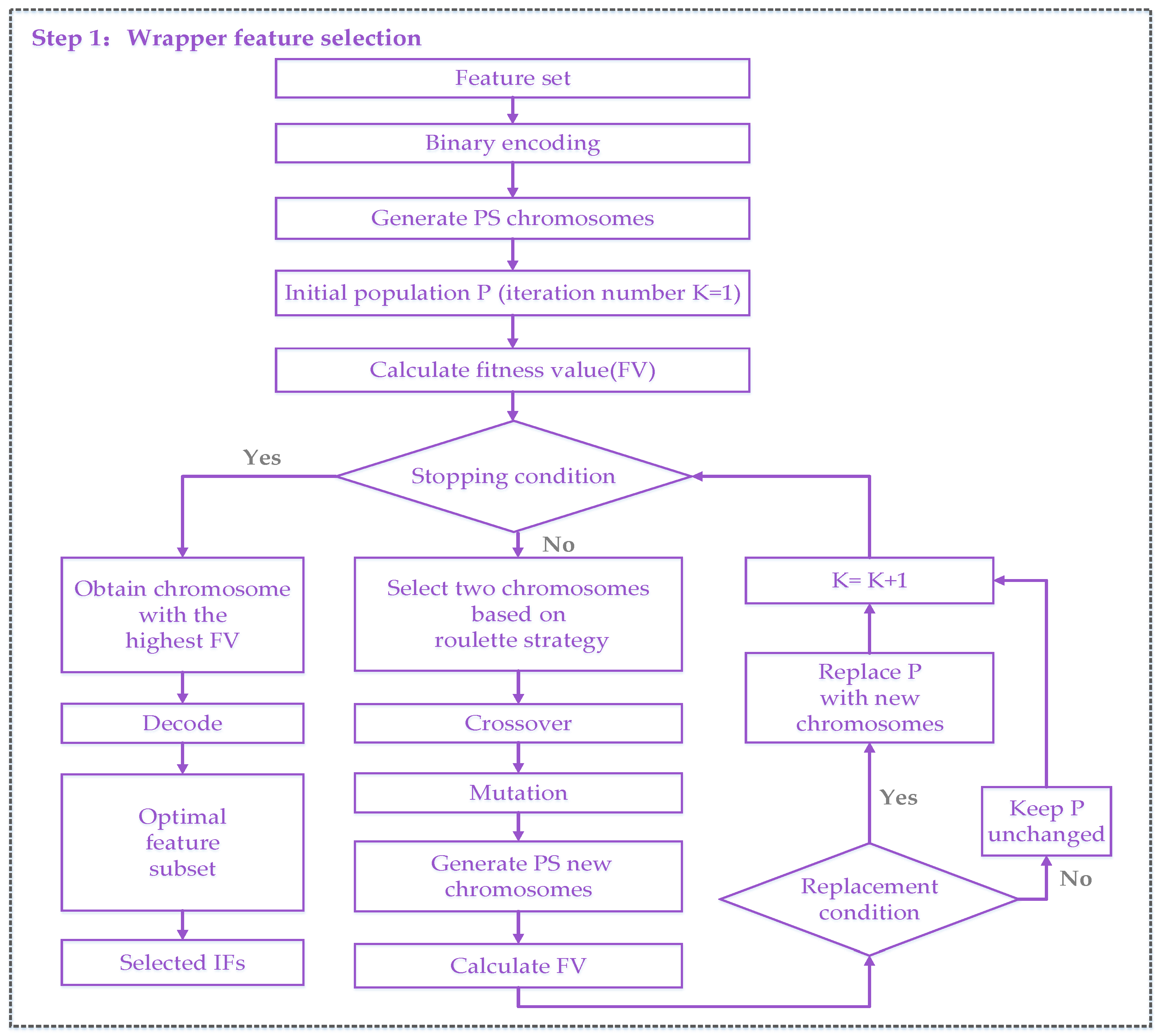
3.1. Wrapper Feature Selection

Feature selection that aims to select significant and non-redundant IFs of RECL is an essential step before the establishment of MLR-based explanatory model in order to ensure the model reliability. To fill the gap that most feature selection methods in relevant researches are merely able to identify the linear relationship, WFS combining GA with MLR is proposed in this paper to better figure out the sophisticated relationship (i.e., linear or nonlinear, functional or non-functional) between IFs and RECL. GA is a search algorithm used to generate new FSs that consists of one or more IFs. MLR is the modeling algorithm used to score these FSs.

The reasons for using GA and MLR are illustrated as follows. First of all, an exhaustive search is simple but time-consuming when the number of selectable IFs is too large. GA is more effective in high-dimensional search spaces, which has already been successfully applied in many fields such as biology and engineering science [25]. Second, MLR based explanatory model is a nonlinear probability model, which is good at illustrating the nonlinear relationship between IFs and RECL. Several key steps of WFS algorithm are shown in the following three sections.

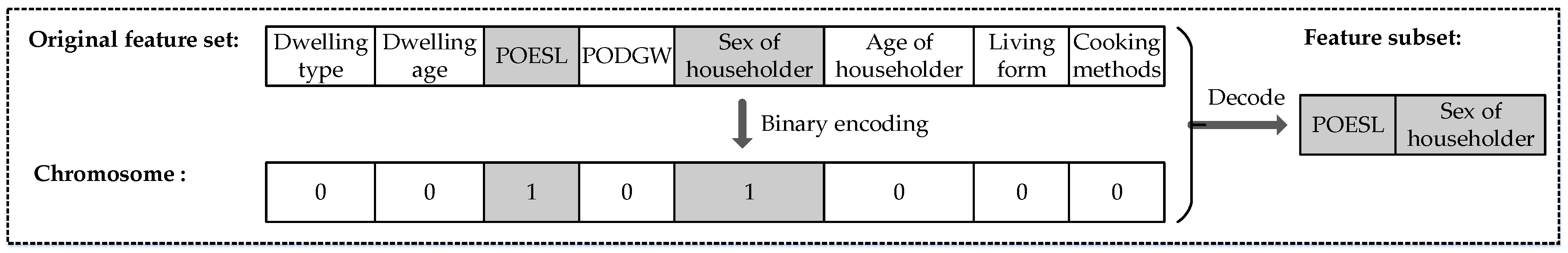
3.1.1. Chromosome Encoding

A set of M selectable IFs is mapped to a numeric string via binary coding. Thus there correspondingly exists M genes coded by binary digits in the chromosome, where 0 means “removing IFs” and 1 means “selecting IFs”. For example, the original feature set in Figure 4 consists of eight alternative IFs. The chromosome coded by “00101000” means that the third and fifth IFs are selected.

3.1.2. Fitness Calculation

Figure 5 shows the detail calculation process of the fitness values (FVs) of chromosomes. First, a classifier is established based on MLR. Then the forecasting accuracy of the classifier verified by 5-fold cross validation is regarded as FV.

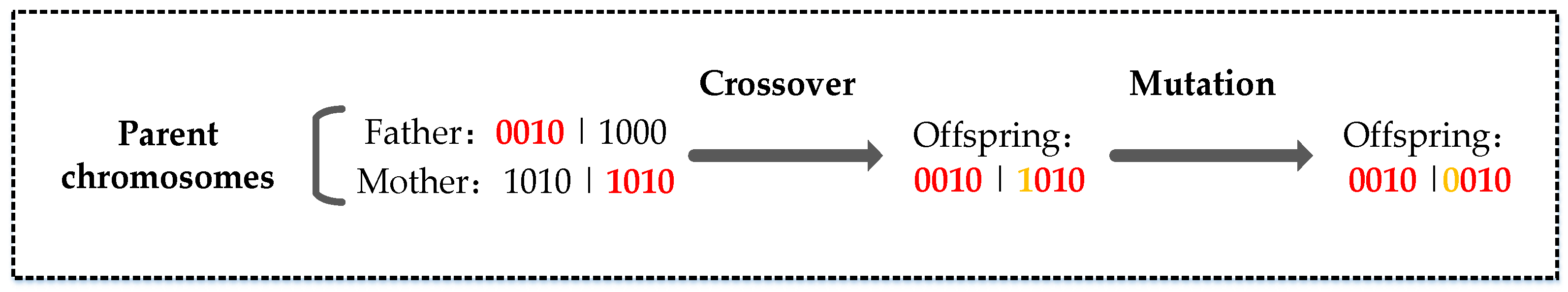
3.1.3. Selection, Crossover and Mutation

The selection principle of parent chromosomes for the generation of new chromosomes should ensure that the chosen probability of chromosomes with higher FVs is larger. Therefore, roulette strategy is applied in WFS algorithm and its detail is shown as follows:

• Calculate the chosen probability p_i of the chromosome C_i by Equation (1), where fitness (C_i) is the FV of the chromosome C_i. This equation shows that the larger the FV of a chromosome, the higher its probability of being selected:

  $$p_i=\mathrm{fitness}(C_i)/{\displaystyle \sum _{i=1}^{PS}\mathrm{fitness}(C_i)}$$

  (1)
• Calculate the accumulative probability of the chromosome C_i by Equation (2), where PP₀ = 0.

  $${PP}_i={\displaystyle \sum _{j=1}^i{p}_i}\left(i=1,\dots ,PS.\right)$$

  (2)
• Generate a random number r within [0, PP_ps].
• Select the chromosome C_i so that PP_i−1 < r < PP_i.

Figure 6 shows that one-point crossover and one-point mutation is applied to the WFS algorithm. Parent chromosomes exchange half of each other’s chromosomal genes during crossover operation to reproduce a new chromosome (i.e., offspring). Then mutation operation further changes one of these genes.

3.2. Maximal Information Coefficient

MIC is utilized to verify the validity of WFS for selecting IFs. The MICs between selected IFs and RECL are calculated to figure out whether these IFs have significant effects on RECL. Meanwhile, the MICs between removed IFs and selected IFs are also calculated to verify the multiple correlations among them. Compared to other commonly used measures (e.g., Pearson coefficient) of the association between two variables, MIC proposed by Reshef et al. [26] is better at identifying a wide range of sophisticated relationships (i.e., linear or nonlinear, functional or non-functional). In addition, MIC is calculated based on mutual information theory and further normalized into a range between 0 and 1. The higher MIC indicates that two studied variables are highly relevant, whereas the MIC of two completely independent variables is close to zero. Some concepts related to MIC are introduced as follows. More detailed descriptions about the theory of MIC can be found in the literature [26].

Intuitively, MIC is based on the idea that if there is a relationship between two variables, various grids can be drawn in the scatter plot of the two variables. These grids partition the data in the scatter plot so that some of the grids are empty and some of them contain points in the scatter plot. When the resolution of the grid is gradually increased, the maximum mutual information that occurs at each resolution can be calculated by the number of points in the grid. The maximum mutual information calculated over the grids with different resolution is normalized to ensure a fair comparison between these grids.

Given a finite set $D=\left\{\left(a_1,b_1\right), \dots ,\left(a_n,b_n\right)\right\}$ whose elements are two dimensions data points, we consider one of the dimensions as x-values and the other as y-values. Then a scatter plot can be drawn when taking x as abscissa and y as ordinate. Suppose x-values is divided into x bins and y-values into y bins, this type of partition is called x-by-y grid G_x,y. Let $D|G_{x,y}$ represent the distribution of D divided by one of the x-by-y grids G_x,y. $\left\{p_0,p_1, \dots ,p_x\right\}$ represents the division point on the axis of the abscissa, where $p_0{=a}_1$ and $p_x{=a}_n$. $\left\{q_0,q_1, \dots ,q_y\right\}$ represents the division point on the axis of the ordinate, where $q_0{=b}_1$ and $q_y{=b}_n$. Differently partitioned grids G_x,y with the same resolution of x-by-y can be obtained by changing the values of $\left\{p_0,p_1, \dots ,p_x\right\}$ and $\left\{q_0,q_1, \dots ,q_y\right\}$.

● Characteristic matrix

Elements m_x,y in the characteristic matrix $\mathrm{M}\left(D\right)=\left[m_{x,y}\right]$ are normalized to achieve a fair comparison between grids G_x,y with different resolutions via the following equations. $I\left(D|G_{x,y}\right)$ is the mutual information of two studied variables a and b over differently partitioned grids G_x,y with the same resolution of x-by-y:

$$m_{x,y}=\max \left\{I\left(D|G_{x,y}\right)\right\}/\log \left(\min \left\{x,y\right\}\right)$$

(3)

● Maximum information coefficient

The MIC of two studied variables a and b is the maximum element in the characteristic matrix M(D). As the upper bound of resolution, B(n) is equal to n^0.6, where n is the sample size.

$$\mathrm{MIC}\left(D\right)=\underset{\mathrm{xy}<B\left(n\right)}{\max }\left\{\mathrm{M}\left(D\right)\right\}$$

(4)

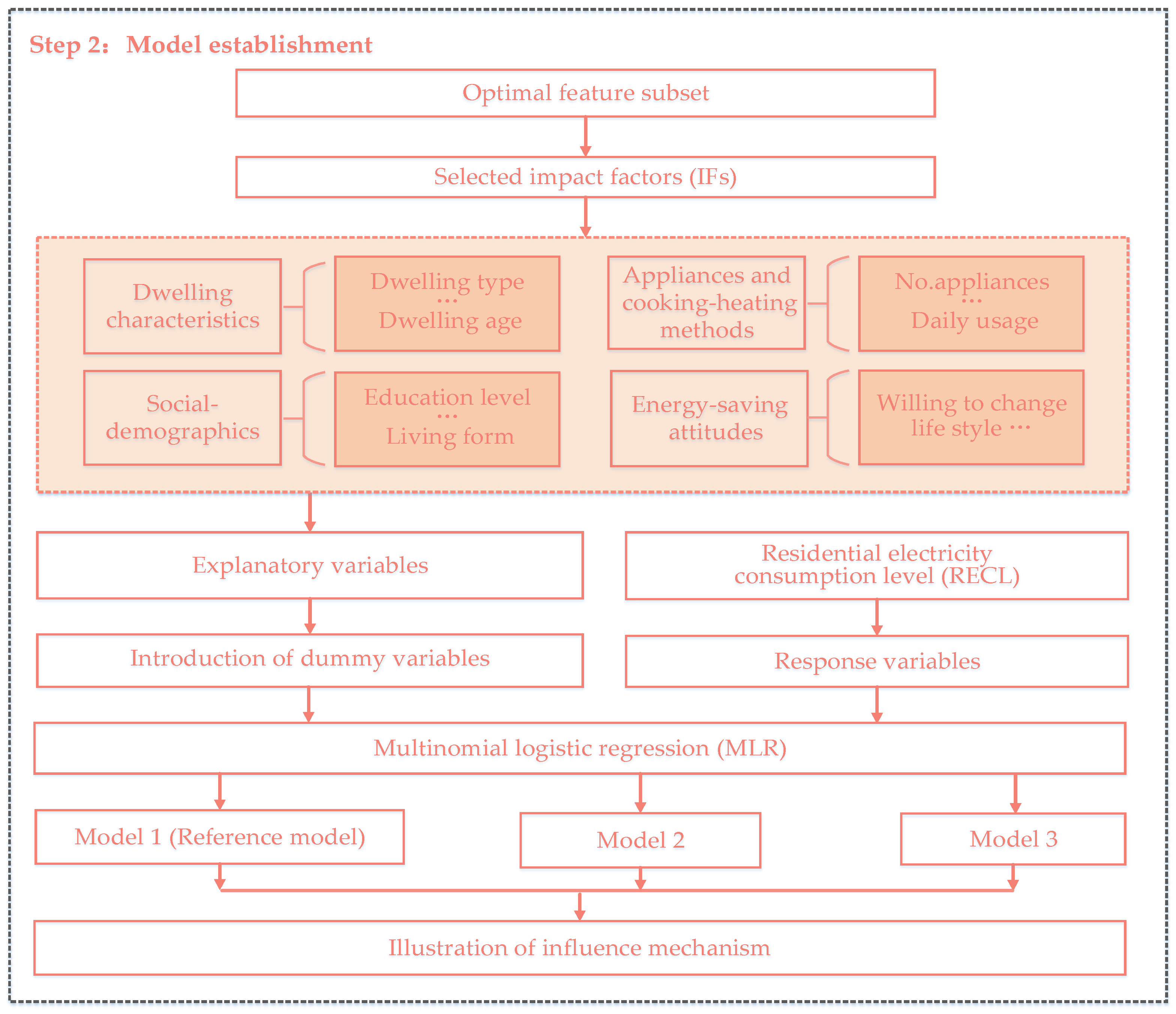
3.3. Multinomial Logistic Regression Model

Different from the common used black-box models such as artificial neural network [27], a regression model (e.g., MLR) can be utilized to explain the relationship between response variables and explanatory variables. In addition, MLR model is a nonlinear probability model applied to predict the probabilities of different possible outcomes of a categorically distributed response variable, given a set of categorical-valued explanatory variables. Compared to other regression methods such as linear regression, the obvious advantage of MLR is that it has fewer basic assumptions such as normal distribution and equal variance. Given the application and advantage of MLR, MLR is adopted in our study to establish an explanatory model for IF analysis of RECL.

As mentioned in Section 2.2, the response variable in our study has three possible outcomes, namely Level 1, Level 2 and Level 3. In addition, Level 1 is considered as the reference category in MLR model. Thus all the coefficients of Model 1 are zero (i.e., g_1i = 0). Two non-redundant sub-models are constructed as follows. With the assumption that there are a total of M categorical explanatory variables, each explanatory variable in regression equation is replaced by several dummy variables based on the replacing methods mentioned in Section 2.2.

● Model 2

$$\begin{array}{l}{g}_{2i}=\ln \frac{P(Y_i=\mathrm{Level}2)}{P(Y_i=\mathrm{Level}1)}\\ ={\alpha }_2 +{\beta }_{21\left(1\right)}{X}_{1i\left(1\right)}+{\beta }_{21\left(2\right)}{X}_{1i\left(2\right)}+\cdot \cdot \cdot +{\beta }_{21\left(N_1\right)}{X}_{1i\left(N_1\right)}+{\beta }_{22\left(1\right)}{X}_{2i\left(1\right)}+{\beta }_{22\left(2\right)}{X}_{2i\left(2\right)}+\cdot \cdot \cdot +{\beta }_{22\left(N_2\right)}{X}_{2i\left(N_2\right)}\\ + \cdot \cdot \cdot +{\beta }_{2M\left(1\right)}{X}_{Mi\left(1\right)}+{\beta }_{2M\left(2\right)}{X}_{Mi\left(2\right)}+\cdot \cdot \cdot +{\beta }_{2M\left(N_M\right)}{X}_{Mi\left(N_M\right)}\end{array}$$

(5)

● Model 3

$$\begin{array}{l}{g}_{3i}=\ln \frac{P(Y_i=\mathrm{Level}3)}{P(Y_i=\mathrm{Level}1)}\\ ={\alpha }_3 +{\beta }_{31\left(1\right)}{X}_{1i\left(1\right)}+{\beta }_{31\left(2\right)}{X}_{1i\left(2\right)}+\cdot \cdot \cdot +{\beta }_{31\left(N_1\right)}{X}_{1i\left(N_1\right)}+{\beta }_{32\left(1\right)}{X}_{2i\left(1\right)}+{\beta }_{32\left(2\right)}{X}_{2i\left(2\right)}+\cdot \cdot \cdot +{\beta }_{32\left(N_2\right)}{X}_{2i\left(N_2\right)}\\ + \cdot \cdot \cdot +{\beta }_{3M\left(1\right)}{X}_{Mi\left(1\right)}+{\beta }_{3M\left(2\right)}{X}_{Mi\left(2\right)}+\cdot \cdot \cdot +{\beta }_{3M\left(N_M\right)}{X}_{Mi\left(N_M\right)}\end{array}$$

(6)

where for each customer $i\left(i=1,2,3,\dots ,3311\right)$, $Y$ is response variable, $X_{1i\left(1\right)}$, $X_{1i\left(2\right)}$, …, $X_{1i\left(N_1\right)}$, $X_{2i\left(1\right)}$, $X_{2i\left(2\right)}$, …, $X_{2i\left(N_2\right)}$, …, $X_{Mi\left(1\right)}$, $X_{Mi\left(2\right)}$, …, $X_{Mi\left(N_M\right)}$ are dummy variables transformed from categorical explanatory variables $X_1$, $X_2$, …, $X_M$ in turn. ${\alpha }_2$, ${\beta }_{21\left(1\right)}$, …, ${\beta }_{2M\left(N_M\right)}$ and ${\alpha }_3$, ${\beta }_{31\left(1\right)}$, …, ${\beta }_{3M\left(N_M\right)}$ are respectively the estimated coefficients of Model 2 and Model 3. $N_1$, $N_2$, …, $N_M$ represent the number of dummy variables of categorical explanatory variable $X_1$, $X_2$, …, $X_M$ in turn. The regression coefficients $\beta$ of MLR model directly determine relative odds ratio (ROR, i.e., the EXP value) involved in classification of customer’s RECL. The ROR of an event is defined as the probability of the event occurring divided by the probability that the event will not occur. As for the “apartment” dummy variable mentioned in Section 2.2, the event specifically refers to the customer who lives in an apartment to use more electricity when compared to the customer who lives in a bungalow. The detail about how to use EXP values to explain the influence mechanism between IFs and RECL will be further presented in Section 4.2. In addition, the RECL classification result of customer i depends on the category with the largest occurring probability, which can be calculated by independent probability model according to Equation (7), where P_i represents the probability of customer i to be a certain category (e.g., Level 1):

$$P_i(Y=\mathrm{Level}j)=e^{g_{ji}}/{\displaystyle \sum _{k=1}^3{e}^{g_{ki}}}\left(j=1,2,3\right)$$

(7)

4. Results and Discussion

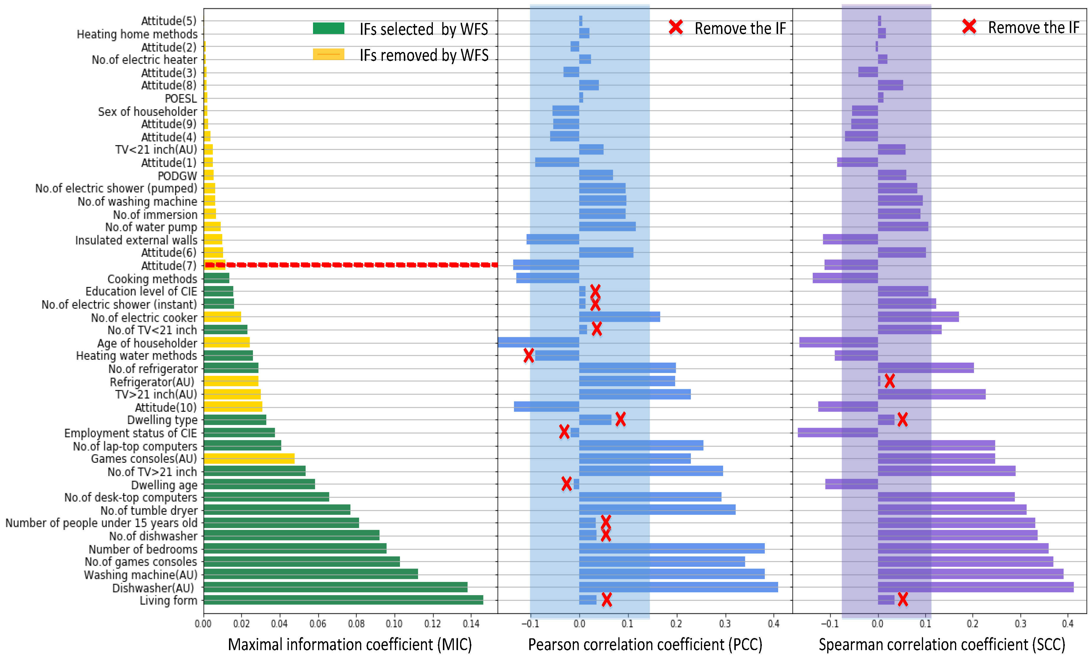
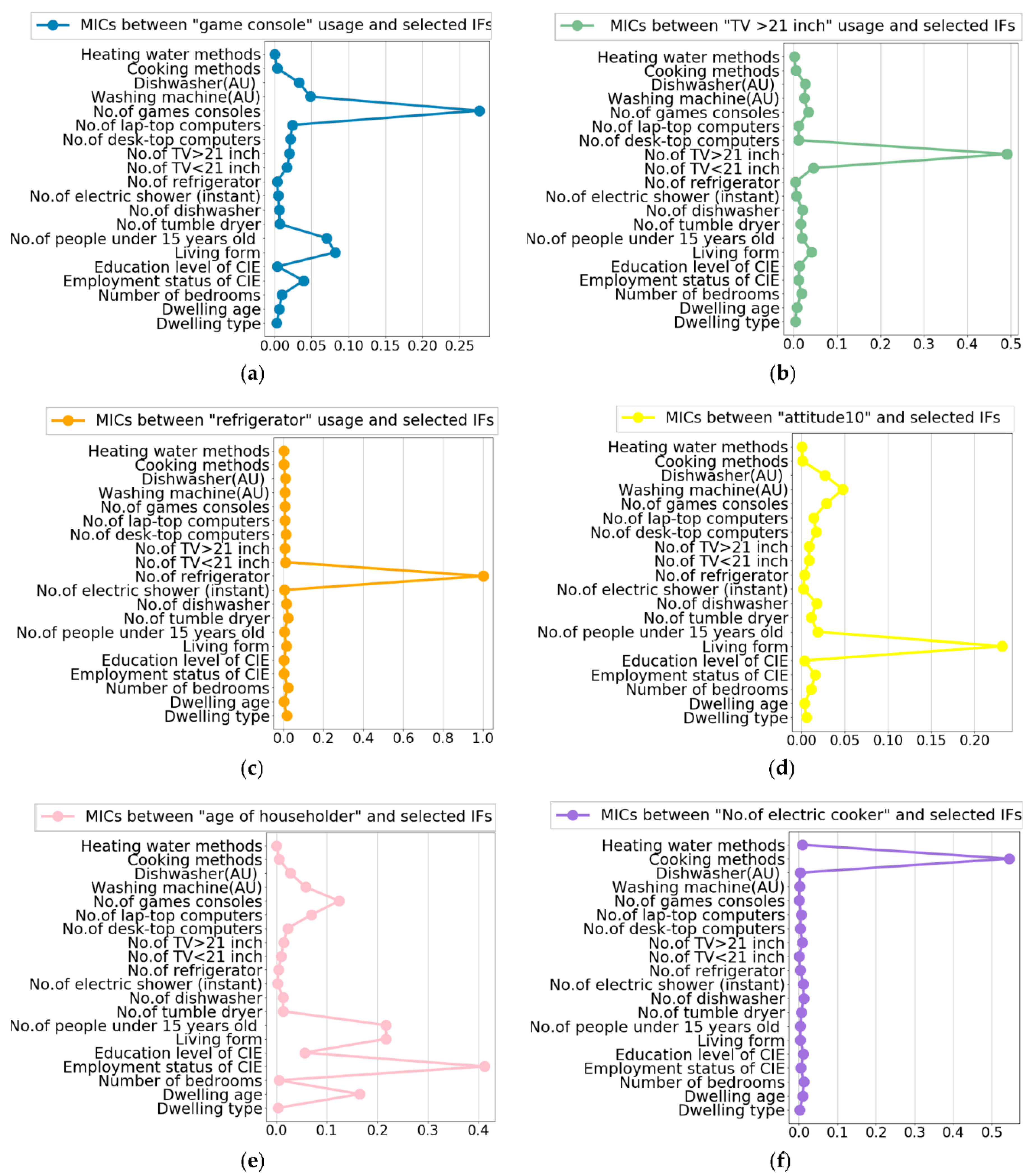
4.1. Validation of Proposed Feature Selection Method

The WFS method is used to identify the significant and non-redundant IFs that are linearly or nonlinearly related to RECL. In this section, the above proposed feature selection method is verified from two aspects. First, WFS is compared with two linear filter methods to verify the WFS’s ability of picking out the significant IFs that are linearly or non-linearly related to RECL. These two linear filter methods are based on different relevance metrics, namely Pearson correlation coefficient (PCC) and Spearman correlation coefficient (SCC). Second, WFS is compared with stepwise linear regression (SLR) to verify WFS’s another ability of identifying the redundant IFs that are linearly or non-linearly related to other IFs.

4.1.1. Comparison between WFS and Linear Filter Methods

In statistics, PCC and SCC are two commonly used relevance metrics. PCC is a measure of the linear correlation between two variables. It has a value between +1 and −1, where 1 is total positive linear correlation, 0 is no linear correlation, and −1 is total negative linear correlation. As for a nonparametric measure of rank correlation between two variables, SCC is equal to the PCC between the rank values of those two variables. It assesses how well the relationship between two variables can be described using a monotonic function. The value of SCC also varies from −1 to 1. The greater the absolute value of SCC, the stronger the monotonic correlation between the two variables. In sum, SCC assesses monotonic relationships (whether linear or not) while PCC merely assesses linear relationships. Different to PCC and SCC, MIC detailed in Section 3.2 is better at identifying a wide range of sophisticated relationships (i.e., linear or nonlinear, functional or non-functional). In addition, the value of MIC is normalized into a range between 0 and 1. The higher MIC indicates that two studied variables are highly relevant, whereas the MIC of two completely independent variables is close to zero.

In this subsection, the above three relevance metrics are used to explain the feature selection results between WFS and linear filter methods. As shown in the first subplot of Figure 7, 20 IFs that marked by green color are selected while the other IFs are removed via WFS. The small MICs also shows that all the yellow marked IFs above the red dotted line have a slight relationship with RECL. Thus the remove of them via WFS is reasonable. However, another six yellow marked IFs under the red dotted line are also removed via WFS although their effects on RECL, indicated by MICs, are not very small. This strange phenomenon is primarily caused by the redundancy among IFs. Redundancy means that IFs are highly correlated and all of them will not simultaneously remain in the regression model in consideration of model reliability. The more detailed explanation is shown in Section 4.1.2. In general, as shown by the MICs, the IFs that are selected by WFS have significant effects on RECL.

The second subplot illustrates the selection results of PCC based linear filter method (PCCLF). The value range of PCC restricted by the blue shadow area is the threshold of this filter. So all the IFs, whose PCCs are covered in this range, are removed. Through the comparison between the first two subplots, the IFs marked by red symbol “×” in the second subplot is falsely removed. This is because the PCCLF is merely able to identify the linear relationship so that it mistakenly judges that the red “×” marked IFs have negligible relationship to RECL. In addition, PCCLF just set a selecting threshold but doesn’t assess the redundancy among IFs. For example, “No. of electric cooker” is redundant but still remain by PCCLF. The selection results of SCC based filter method and the explanation behind are similar to the PCCLF and we will not repeat them here.

According to the above comparison, it can be concluded that WFS is superior to the two linear feature selection methods. The WFS can correctly remove the insignificant IFs of RECL and identify the redundancy among IFs while the two linear feature selection methods cannot.

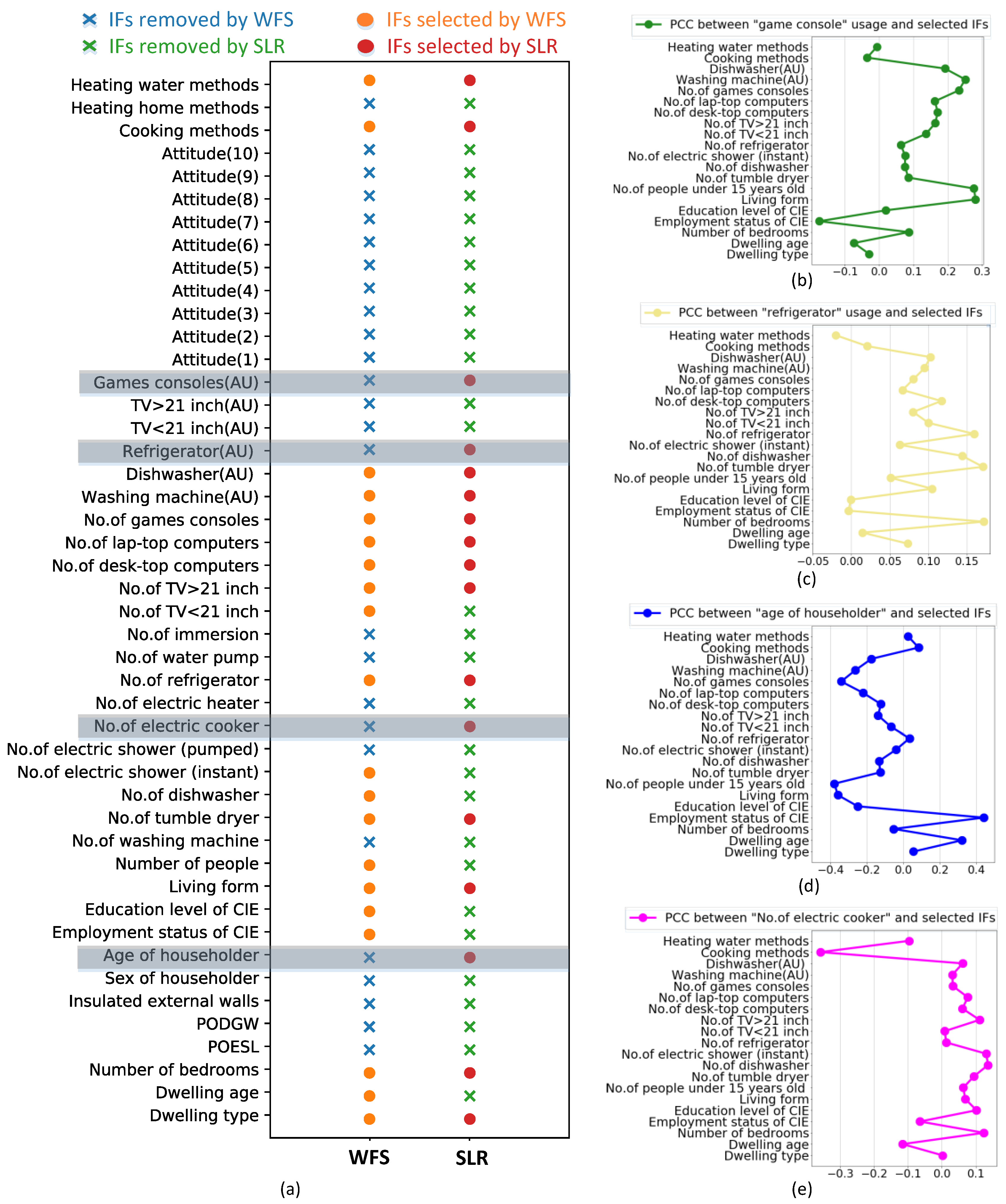
4.1.2. Comparison between WFS and SLR

In this subsection, the results of feature selection is compared between WFS and SLR to verify WFS’s another ability of identifying the redundant IFs that are linearly or non-linearly related to other IFs. First of all, the MICs between the six redundant IFs (mentioned in Section 4.1.1) and selected IFs is presented in Figure 8. The corresponding explanations are illustrated as follows.

In graph (a), the highest MIC shows that game consoles usage is significantly related to the total number of game consoles. As proposed in the previous literature, appliances ownership alone will not directly affect electricity consumption [28]. It is appliance usage together with ownership that affects the consumption pattern of residents. Due to the internal correlation between the two factors, one of them is removed by WFS. As shown in graph (b) and (c), “TV > 21 inch (AU)” and “Refrigerator (AU)” variables are also removed by WFS because of the same reason.

Graph (d) indicates that “Attitude (10)” about whether you are able to let the people you live with reduce their electricity usage has a close relationship with living form. From the psychological perspective, the electricity consumption behavior of a person is driven by many complex psychological factors such as attitudes [29]. The encouragement of electricity conservation from others will unconsciously change persons’ energy saving attitudes and further affect their consumption behaviors [30]. Nevertheless, the influence of his attitudes on others consumption behaviors would be constrained if a person lives alone. Given the internal correlations between “Attitude (10)” and “Living form” variables, one of them is removed by WFS.

Differently, “Age of householder” variable is simultaneously related to several factors, namely “Employment status of CIE”, “Living form” and “No. of people under 15 years old”. Although “Age of householder” variable is removed by WFS because of redundancy, previous studies indicated that the age of the household responsible person (HRP) did affect household’s electricity use [9,17,25,26]. Majority literature found that the HRPs in the range of 46 and 65 years old used more electricity than other age groups [9,25,26]. This could be attributed to the fact that middle-aged HRPs usually have more children, which results in longer occupancy hour and a larger number of appliance equipped room [30]. Households with younger HRPs (aged between 18 and 35 years old) and older HRPs (aged over 65 years) consume less electricity [10,21]. Although older people retired usually have longer occupant time during the day, their electricity consumption is not very high due to their strong energy-saving awareness. As for younger people, they spend less time at home due to a full-time job, which also results in less electricity consumption.

Graph (f) indicates that “No. of electric cooker” is related to “Cooking methods”. Households owning one or more electric cooker are more likely to be high electricity consumers Furthermore, dwellings using electricity to cook tends to use more electricity than that using other kinds of energy (e.g., oil and gas) to cook. However, the influence of cooking methods on electricity consumption will be weakened a lot when the families have no electric cooker. Due to the internal correlation between the two factors, one of them is also removed by WFS.

Although these six IFs are redundant, the comparison results in the graph (a) of Figure 9 shows that SLR fails to remove four redundant Ifs (i.e., “game console” usage, “refrigerator” usage, “age of householder” and “No. of electric cooker”). In other words, unlike WFS, SLR is not good at identifying the nonlinear redundancy. This is because SLR is a method of fitting multiple linear regression models in which the choice of predictive variables is carried out by an automatic procedure. In each step, a variable is considered for addition to or subtraction from the set of explanatory variables based on the pre-specified criterion called adjusted R2. Thus SLR is limited to identification of linear redundancy. In graphs (b)–(e) of Figure 9, the PCCs between these four IFs and selected IFs are small. All the absolute values of these PCCs are less than 0.5, showing the slight linear relationship between these four IFs and selected IFs. So these four IFs are mistakenly selected by SLR. In sum, when compared to SLR, WFS shows the good ability of identifying the redundant IFs that are linearly or non-linearly related to other IFs.

4.2. Illustration of Influence Mechanism between IFs and RECL

The first subplot of Figure 7 shows important information as follows. Firstly, “Living form”, “Number of bedrooms”, “Number of people under 15 years old”, “Dwelling age”, “Number of appliances (i.e., game consoles, dishwasher, tumble dryer, desktop computers and TV > 21 inch)”, and “Usage of appliances (i.e., dishwasher and washing machine)” are all significantly related to RECL. Secondly, “Employment status of CIE”, “Dwelling type”, “Attitude (10)”, “Heating water methods”, “Age of householder”, “Education level of CIE”, “Cooking methods”, “Number of appliances (i.e., laptop computers, refrigerator, TV < 21 inch, electric cooker and instant electric shower)”, and “Usage of appliances (i.e., game consoles, TV > 21 inch and refrigerator)” all have smaller effect on RECL. Thirdly, the IFs above the red dotted line almost have no effect on RECL. MIC can only calculate the association degree between two IFs but fails to figure out the specific influence mechanism between them.

Table 2. Overview of multinomial logistic regression results and MICs.

Residential Characteristics (IFs) b	Model 2 a		Model 3 a		MIC
	B2	ExpB2	B3	ExpB3
Category1: Dwelling characteristics
Dwelling type (Ref: Bungalow)					0.033
(1) Apartment	−1.024	0.359	−1.508	0.221
(2) Semi-detached	−0.327	0.721	−0.586	0.556
(3) Detached	−0.185	0.831	−0.131	0.878
(4) Terraced	−0.409	0.664	−0.629	0.533
Dwelling age (Ref: 40 years +)					0.058
(1) 0 ~ 20 years	−0.536	0.585	−0.583	0.558
(2) 20 ~ 40 years	−0.124	0.883	−0.228	0.796
No. of bedrooms (Ref: 5+)					0.096
(1) 1	−1.593	0.203	−1.610	0.200
(2) 2	−0.510	0.610	−1.159	0.314
(3) 3	−0.186	0.830	−0.661	0.516
(4) 4	0.099	1.105	−0.186	0.830
Category2: Socio-demographic
Employment status of CIE (Ref: Retired or keeper)					0.038
(1) Employee	−0.401	0.670	−0.232	0.793
(2) Self-employed	−0.203	0.816	0.017	1.107
(3) Unemployed	−0.378	0.685	−0.332	0.717
Education level of CIE (Ref: Third level)					0.016
(1) Not educated	0.249	1.283	1.039	2.827
(2) Primary	−0.240	0.787	−0.634	0.530
(3) Second level	−0.463	0.629	−0.762	0.467
Living form (Ref: With adults and children)					0.147
(1) Live alone	−1.520	0.219	−1.134	0.332
(2) All adults	−0.445	0.641	0.065	1.067
No. of people under 15 years old (Ref: 4+)					0.082
(1) 0	−0.526	0.590	−0.626	0.535
(2) 1	−0.520	0.594	−0.420	0.657
(3) 2	−0.012	0.988	−0.112	0.894
(4) 3	−0.130	0.878	−0.030	0.970
Category3: Appliance and Cooking -heating methods
No. of tumble dryer(Ref: 2)					0.077
(1) 0	−0.613	0.542	−0.713	0.490
(2) 1	−0.102	0.903	−0.201	0.818
No. of dishwasher(Ref: 2)					0.092
(1) 0	−0.378	0.685	−0.481	0.618
(2) 1	−0.012	0.988	−0.154	0.857
No. of electric shower (instant) (Ref: 2+)					0.016
(1) 0	−0.834	0.434	−0.923	0.397
(2) 1	−0.634	0.530	−0.682	0.505
(3) 2	−0.234	0.791	1.019	2.77
No. of refrigerator(Ref: 2+)					0.029
(1) 0	−0.532	0.587	−0.532	0.587
(2) 1	−0.220	0.802	−0.220	0.802
(3) 2	1.399	3.816	1.399	3.816
No. of TV’s < than 21 inch(Ref: 3+)					0.023
(1) 0	−1.321	0.266	−0.975	0.377
(2) 1	−0.912	0.407	−0.856	0.424
(3) 2	−0.754	0.470	−0.634	0.530
(4) 3	−0.323	0.724	−0.244	0.783
No. of TV’s > than 21 inch(Ref: 3+)					0.054
(1) 0	−1.227	0.293	−1.374	0.253
(2) 1	−0.745	0.475	−0.643	0.526
(3) 2	−0.803	0.448	−0.518	0.596
(4) 3	−0.568	0.567	−0.391	0.676
No. of desk-top computers(Ref: 3+)					0.066
(1) 0	−0.890	0.411	−0.719	0.487
(2) 1	−0.234	0.791	−0.412	0.662
(3) 2	−0.018	0.982	−0.230	0.795
(4) 3	0.012	1.102	0.031	1.031
No. of lap-top computers(Ref: 3+)					0.041
(1) 0	0.917	2.501	0.812	2.252
(2) 1	1.063	2.896	1.023	3.013
(3) 2	1.210	3.354	1.254	3.504
(4) 3	1.890	6.617	2.012	7.478
No. of games consoles(Ref: 3+)					0.103
(1) 0	−0.523	0.593	−0.782	0.457
(2) 1	−0.322	0.725	−0.423	0.655
(3) 2	−0.345	0.708	−0.243	0.784
(4) 3	0.123	1.131	−0.102	0.903
Washing machine(AU) (Ref: 3 loads+)					0.112
(1) Less than 1 load	0.226	1.254	−0.760	0.468
(2) 1 load	0.467	1.596	−0.056	0.945
(3) 2–3 loads	1.071	2.918	0.611	1.842
Dishwasher(AU) (Ref: 3 loads+)					0.138
(1) Less than 1 load	−0.632	0.532	−0.731	0.481
(2) 1 load	−0.456	0.634	−0.343	0.710
Cooking methods (Ref: Use other energy)					0.014
(1) Use Electricity	0.512	1.669	0.910	2.484
Heating water methods (Ref: Use other energy)					0.026
(1) Use Electricity	0.217	1.242	0.434	1.543

^a Level 1 is regarded as the reference category in MLR model. The numbers in column B2 and B3 are respectively the estimated coefficients of dummy variables in Model 2 and Model 3. These coefficients satisfy the equation ExpB₂ =$e^{B_i}$(i = 2,3); ^b For each IF, dummy variables numbered by (1), (2)… are introduced. Ref is the abbreviation of reference variable.

clearly presents the regression results of MLR model, which is used to explain how these selected IFs (i.e., residential characteristics) affect RECL. The numbers in column B₂ and B₃ are respectively the estimated coefficients of dummy variables in Model 2 and Model 3 mentioned in Section 3.3. For dummy variables, their EXP values are calculated according to their corresponding regression coefficients and the Equation ${ExpB}_i=e^{B_i}（i=2,3）$.

An EXP value of 1 indicates that households with given residential characteristics are just as likely to be high electricity consumers as the households in the reference group. An EXP value greater than 1 indicates a higher probability that a household would be a high user compared to the reference group, whereas an EXP value below 1 indicates that the probability is lower than for the reference group. In addition, the higher the EXP value, the more likely it is that the households would be high consumers compared to the reference group. Detailed influence mechanism is described as follows.

4.2.1. Dwelling Characteristics

With respect to dwelling characteristics, the small MICs in Figure 7 show that energy-saving lights, double-glazed window and external walls have a negligible effect on electricity use. Previous studies also found that there was no significant relationship between the presence of energy-saving lights and electricity use, because no clear reduction in electricity consumption occurred when energy-saving lights were installed in dwellings [31]. This may be caused by the small proportion lighting consumption represents in total domestic electricity use. Therefore it is irrational to expect an obvious impact of energy-saving lights on electricity demand.

As for insulation decoration such as double-glazed window and external walls, earlier studies reported inconsistent results about their influence on electricity usage. Some found that the insulation decoration was helpful for the reduction in electricity use, whereas some others found no relationship between them [21]. Another study even revealed that well-insulated dwellings tended to use more electricity [32]. In fact, the factors related to insulation decoration are very important when looking at the electricity demand for heat loss [33]. However, our study finds no significant effects of such IFs on electricity use, which may be caused by the small proportion (about 7.2% as shown in Table 1) of electrically heated households in our studied sample.

Compared to other dwelling characteristics, the biggest MICs in Table 2 show that the number of bedrooms plays the most significant role in the variation of electricity consumption. The EXP values of this IF in Table 2 indicate that dwellings with two or more bedrooms are more likely to be the high electricity demand group. The significantly positive relationship between the numbers of bedrooms and electricity use also has been supported by other scholars who believe that the more the number of rooms, the more electricity usage [34]. Researchers explained the positive relationship between the number of rooms and electricity use by arguing that dwellings with more rooms always had more appliances for entertainment and room lighting [10].

Based on the comparison among the EXP values of dwelling type’s dummy variables, it is obvious that households living in bungalows consume more electricity than those living in detached, semi-detached and terraced dwellings. Additionally, households living in apartments consume the minimum electricity. This is because apartments have a lower detached degree and less exposed walls, which should reduce electricity heating demand. Similar results were also found in numerous studies, indicating that larger dwelling’s detached degree and exposed wall’s surface increased the electricity demand for cooling and heating [9,26,29]. In addition, some researchers suggested that the influence degree of dwelling type on power usage relied on floor area, because a smaller floor area restricted the exposed surface and thus decreased the space cooling and heating requirements in electrically heated rooms [35].

The EXP values growing with dwelling age reveals a tendency in older dwellings to consume more electricity. Earlier studies also observed a decrease of electricity demand in newer houses with improved insulation and energy-efficient appliances [24,30,31,32,33]. Some studies found the opposite results that newer houses consume more electricity than older ones due to the penetration of high-consumption appliances such as air conditioning [36,37,38,39]. However, some found no significant effect of dwelling age on electricity usage when the studied sample was under the enforcement of dwelling regulations [21]. Such regulation made the physical conditions of dwellings constructed in different years same. In sum, the influence degree of dwelling age on power usage is affected by other factors such as policy intervention and appliance performance.

4.2.2. Social Demographics

As for social demographics, two IFs (i.e., the age and sex of householder) are removed due to different reasons. The remove of former IF is caused by its multiple correlations with other factors, the detailed explanation of which has been given in Section 4.1. But the remove of latter IF is due to its small association with RECL. This is also supported by Brounen et al. [35] who assert that gender had no effect on the electricity use for thermal comfort. However, others revealed that the electricity consumption behaviors varied between male and female due to different preference for physiological temperature [35,36,40]. These various results are primarily explained by the fact that scholars carried out related experiments in regions where the climate is different, which results in different thermal sensation difference between males and females [41].

Compared to other social-demographic factors, the MIC of the living form (i.e., live alone or not) is highest in Table 2, indicating that living form has a close relationship with electricity consumption. Meanwhile, the related EXP values indicate that households with more people tend to use more electricity than those with only one person. Many previous studies also found similar results by explaining that growth in the number of occupants would increase the electricity demand of appliance [17,24,29,30,32]. For example, households with more members will undoubtedly generate more dirty laundry each week and require more showers and so use more electricity for washing machines, tumble dryers and electric showers.

The number of people under 15 years old is the second significant factor of RECL among social-demographical factors. The EXP values show that households with two or more children tend to use more electricity, which is also found in earlier studies [30,32,33]. This result is primarily because children are less conscious of the electricity they use and thus consume more electricity for IT and entertainment appliances in their spare time [30]. Moreover, children’s age also affects the relationship between the number of children and electricity consumption. Some researchers indicated that the presence of children under 3 had no significant impact on power usage whereas the presence of children older than 3 played a more important role in it [10].

Concerning employment status of CIE, the EXP values of employed, self-employed and unemployed person are all smaller than 1 when the “Retired or keeper” is considered as a reference variable. This result indicates that households with retiree or keeper are more likely to be the high electricity consumers than that with an employee or the jobless. Because retiree or keeper has a longer time to stay at home during the day than employee or the jobless, which should increase the frequency of using appliances for housework and entertainment [10].

The EXP values of educational level in Table 2 shows that the households occupied by intellectuals tend to consume less electricity than that occupied by the uneducated. Similarly, some studies also found a significant decrease in domestic electricity consumption when education level of family members increased [9]. This is because intellectuals always have the high energy-saving consciousness to protect the environment, as well as the strong economic strength to purchase expensive energy-star appliances.

4.2.3. Appliance and Cooking-Heating Methods

During the WFS process, 11 IFs related to appliance were removed and the other 10 IFs were selected. The MLR model further shows that the ownership and usage of appliance also have an influence on RECL. Specifically speaking, the EXP values in Table 2 verify that growth in the number of appliances, as well as longer duration use of the appliance, will increase the probability to use more electricity.

As for the appliance category related to dishwashing and drying, the EXP values reveals that households with one or more tumble dryers and dishwashers tend to use more electricity. In addition, the number of tumble dryers and dishwashers might also be related to the household size [28]. Households with more family members may have more dirty clothes and dishes, so more tumble dryers and dishwashers are needed to do the housework.

Regarding the wet appliance category, as the number of instant electrical shower increased, so too do the likelihood of high electrical energy demand. The electrical shower is one of the highest power consumption appliances in households despite its short time of duration usage. Thus, it is understandable that dwellings with one or more electrical showers tend to use more electricity.

The EXP values also show that the presence of cooling appliances such as refrigerator is undoubtedly responsible for high electricity demand. As one of the commonly used appliances, refrigerator usually turns on during the year, which better explains the above results.

As for the entertainment appliance category, the EXP values in Table 2 reveal that the more number of entertainment appliances, the higher the probability of households to be high electricity consumers. Similar to the earlier study [31], our results find that the number of TVs is positively related to domestic electricity demand. On the one hand, TVs may be simultaneously used by occupants preferring different TV programs. On the other hand, TV can also be used as the display screen for video game console or desktop computer. These two reasons explain the positive influence of TVs on electricity use. Furthermore, the comparison between the MICs of TVs with different size indicates that TV larger than 21 inch has a greater influence on power usage than TV smaller than 21 inch. Regarding the number of game console, its EXP values show that households owning one or more game consoles are always inclined to consume more electricity. Also, the influence of game consoles ownership may be strengthened by the presence of children, because they are the main group for playing video games [9,26].

In the IT appliance category, the EXP values show that the growing number of desktop or laptop computers is more likely to result in higher electricity demand. It was also observed by many previous studies [42] that as the number of computers increased, so too did the likelihood of dwellings to be high electricity group. A UK study argued that the positive correlation between IT appliance ownership and electricity use might be caused by the high electricity consumption performance of IT appliance [43]. Moreover, owning a desktop or laptop computer possibly promotes the purchase of other compatible IT appliances (e.g., printers, scanners and routers), which further leads to higher residential electricity consumption [28].

However, appliance ownership only partially reflects the effects of domestic appliances on RECL. It is also essential to take appliance usage into consideration. As for the laundry appliance category, the EXP values show that frequent and long use of washing machine for dirty clothes will certainly increase the electricity demand. Similarly, if households do longer dishwashing via dishwasher, their electricity consumption is also likely to increase. Several researchers believe that both duration and frequency of appliance usage play a role in electricity demand [9,23]. Furthermore, the influence extent of appliances usage on electricity consumption primarily depends on the electricity consumption characteristics of appliances.

When it comes to cooking-heating methods, the EXP values reveal that the households using electricity to cook or heat are about two times more likely to be high electricity consumers than those using other kinds of energy (e.g., oil, gas) to cook or heat.

4.2.4. Attitudes

Except for the IF called “Attitude (10)”, the other nine IFs related to energy-saving attitudes were removed by WFS. In Figure 7, the small MICs of these nine IFs verify their insignificant effects on RECL. This further reveals that the potential gap between energy-saving attitudes and actual behaviors would weaken the influence degree of attitudinal factors on RECL. Furthermore, the influence of “Attitude (10)” on RECL is still unknown as this variable is removed and not contained in the final MLR model. As previously discussed in Section 4.2.1, this factor is highly associated with the living form, which indicates that “Attitude (10) may have an indirect influence on RECL through the living form.

5. Application

The application of our study can be elaborated mainly from two perspectives. One is the standing on stakeholders’ position, and the other focuses on methodology. From the perspective of some stakeholders, a better understanding of the influence mechanism between significant factors and electricity consumption can useful guidance for local governments, electric power companies, and individual households to take effective measures related to electricity. For local governments, inspired by the analysis results, they can intervene in two aspects, namely governmental policy and technological improvement. In the first aspect, the above results show that dwelling characteristics, such as dwelling type and insulation decoration, have significant impacts on the electricity use. This information reminds the government that it is necessary to draw effective building regulations to widely improve energy efficiency of houses. Further, in consideration of the role of social demographics (e.g., employment status and educational level) on electricity use, more effort should be paid on economic development and educational investment. In the second aspect, the close relationship between appliance and electricity use reveals that governments should strengthen the monitoring of energy-saving appliances production technology.

For electric power company, detailed IF analysis of RECL is also helpful for scientific designs of targeted services such as demand response (DR) programs [44]. According to the influence mechanism discussed in this paper, households with different residential characteristics have different electricity consumption level. Thus it is more effective to provide targeted DR programs (e.g., well-designed various pricing mechanisms [45] and feedbacks) for specific residential customers with great potential for electricity reduction [46,47]. Because it is of no use to implement DR programs on the house with no more energy-saving space. And irrational DR programs will destructive the balance between people’s comfortable degree and willingness degree of energy saving. In addition, the knowledge of residential electricity consumption behavior is helpful for the system operators (e.g., transmission system operators and distribution system operators) to achieve the reliable smart residential energy scheduling [48,49,50].

For individual households, they are encouraged to live in the apartments because the above findings show that apartments are the most energy efficient when compared to other dwelling types. Such energy-saving advantage is due to apartment’s smaller detachment degree and exposed surface. Given the significant impact of the appliance on electricity consumption, individuals could decrease their electricity use through changing their habits of using appliance (e.g., turn off the equipment when not use, do housework by hands, reduce the duration of appliance operation). In addition, purchasing energy-star appliances is also suggested.

From the perspective of methodology, a novel WFS is proposed, which can be applied to address the problems of dimension curse and multiple correlations during the establishment of regression model. The solution to the two mentioned problems can guarantee the accurate of estimated coefficients of the regression model, which is also helpful for the reliability of the later statistical analysis. The proposed WFS is different to the previous linear feature selection methods in the current research field of residential electricity analysis. Because WFS is able to identify the significant and non-redundant IFs that are linearly or nonlinearly related to RECL. This WFS model can be applied to other field to carry out feature engineering.

6. Conclusions

In-depth analysis of the influencing mechanism behind residential electricity consumption is helpful for the improvement of energy efficiency. In this paper, a complete research framework is proposed to identity significant impact factors (IFs) of residential electricity consumption level (RECL) and better understand the influence mechanism of IFs on RECL. The framework consists of two steps. First, a novel WFS method is proposed to pick out significant and non-redundant IFs. Second, MLR based explanatory model is further to illustrate how the selected IFs affect RECL. The relevant simulation results is illustrated and discussed as follows.

As for the first step, the WFS is proposed to fill the gap that most previous feature selection methods in current research field are merely able to identify linear relationships. Further, compared to two linear feature selection methods (based on PCC and SCC) and SLR, the simulation results verifies that WFS shows its superiority in identification of nonlinear relationship. In other words, WFS can identify the significant and non-redundant IFs that are linearly or nonlinearly related to RECL while the three methods that are compared to WFS cannot.

With regard to the second step, studied IFs that are included in the explanatory model are divided into four categories including dwelling characteristics, socio-demographics, appliances and cooking-heating methods, and energy-saving attitudes. The relationships between IFs and RECL are summarized as follows. As for dwelling characteristics, dwelling age and the number of bedrooms are found to have a positive impact on electricity usage. Dwelling type also has a close association with the electricity demand for space cooling and heating. For socio-demographics, the employment status, education level, living form and the number of people under 15 years old also influence the RECL in different extent. More specifically, households that have retiree or keeper, persons without formal education or two or more children, are more likely to be the high electricity demand group. In terms of appliances and cooking-heating methods, appliance ownership and usage are also closely related to electricity consumption. The households that supplied by other kinds of energy (e.g., oil, gas) to cook or heat tend to consume less electricity. However, most attitudinal variables have negligible influence on power usage, which may be caused by the potential gap between energy-efficient concepts and actual behaviors.

In our future work, we will focus more on the following four aspects. First, it is important to figure out a rational method that aims to utilize the easily accessible information (e.g., dwelling types, population structure and appliance ownership) to indirectly predict the uneasily accessible information (e.g., the frequency of use of appliances). This can save a lot workload of data collection in the future. Second, besides the study of the relationship between residential characteristics and electricity consumption, another attention should be paid to the interactions among IFs (e.g., how the age of households affects the appliance usage). Third, an inference of residential characteristics based of historical electricity consumption data is a meaningful research direction, which is helpful to further estimate customers’ potential of peak shaving and energy saving under the implement of price based demand response programs. Fourth, another interesting future work is to explore whether the results will change significantly if a “per-capita consumption” is use instead of total house consumption.

References

1. Liu, Y.; Gao, Y.; Hao, Y.; Liao, H. The Relationship between Residential Electricity Consumption and Income: A Piecewise Linear Model with Panel Data. Energies 2016, 9, 831. [Google Scholar] [CrossRef]
2. Oprea, S.-V.; Bâra, A.; Reveiu, A. Informatics Solution for Energy Efficiency Improvement and Consumption Management of Householders. Energies 2018, 11, 138. [Google Scholar] [CrossRef]
3. International Energy Agency. IEA Electricity Information. IEA Stat. 2013, 1–708. [Google Scholar] [CrossRef]
4. Liu, H.; Zhou, S.; Peng, T.; Ou, X. Life Cycle Energy Consumption and Greenhouse Gas Emissions Analysis of Natural Gas-Based Distributed Generation Projects in China. Energies 2017, 10, 1515. [Google Scholar] [CrossRef]
5. Costa, A.; Keane, M.M.; Torrens, J.I.; Corry, E. Building operation and energy performance: Monitoring, analysis and optimisation toolkit. Appl. Energy 2013, 101, 310–316. [Google Scholar] [CrossRef]
6. Doha Amendment to the Kyoto Protocol; United Nations Framework Convention on Climate Change (UNFCCC), Climate Change Secretariat: Bonn, Germany, 2012.
7. Paris Agreement; United Nations Framework Convention on Climate Change (UNFCCC), Climate Change Secretariat: Bonn, Germany, 2015.
8. Centobelli, P.; Cerchione, R.; Esposito, E. Environmental sustainability and energy-efficient supply chain management: A review of research trends and proposed guidelines. Energies 2018, 11, 275. [Google Scholar] [CrossRef]
9. Huebner, G.; Shipworth, D.; Hamilton, I.; Chalabi, Z.; Oreszczyn, T. Understanding electricity consumption: A comparative contribution of building factors, socio-demographics, appliances, behaviours and attitudes. Appl. Energy 2016, 177, 692–702. [Google Scholar] [CrossRef]
10. Jones, R.V.; Fuertes, A.; Lomas, K.J. The socio-economic, dwelling and appliance related factors affecting electricity consumption in domestic buildings. Renew. Sustain. Energy Rev. 2015, 43, 901–917. [Google Scholar] [CrossRef] [Green Version]
11. Bahrami, S.; Sheikhi, A. From Demand Response in Smart Grid Toward Integrated Demand Response in Smart Energy Hub. IEEE Trans. Smart Grid 2016, 7, 650–658. [Google Scholar] [CrossRef]
12. Amini, M.H.; Nabi, B.; Haghifam, M.-R. Load Management Using Multi-Agent Systems in Smart Distribution Network. In Proceedings of the IEEE Power and Energy Society General Meeting (PES), Vancouver, BC, Canada, 21–25 July 2013; pp. 1–5. [Google Scholar] [CrossRef]
13. Bahrami, S.; Wong, V.W.S. Security-Constrained Unit Commitment for ac-dc Grids with Generation and Load Uncertainty. IEEE Trans. Power Syst. 2017, 33, 2717–2732. [Google Scholar] [CrossRef]
14. Chen, Q.; Wang, F.; Hodge, B.M.; Zhang, J.; Li, Z.; Shafie-Khah, M.; Catalao, J.P.S. Dynamic Price Vector Formation Model-Based Automatic Demand Response Strategy for PV-Assisted EV Charging Stations. IEEE Trans. Smart Grid 2017, 8, 2903–2915. [Google Scholar] [CrossRef]
15. Wang, F.; Zhou, L.; Ren, H.; Liu, X.; Talari, S.; Shafie-khah, M.; Catalao, J.P.S. Multi-objective Optimization Model of Source-Load-Storage Synergetic Dispatch for Building Energy System Based on TOU Price Demand Response. IEEE Trans. Ind. Appl. 2017. [Google Scholar] [CrossRef]
16. Wang, F.; Zhen, Z.; Mi, Z.; Sun, H.; Su, S.; Yang, G. Solar irradiance feature extraction and support vector machines based weather status pattern recognition model for short-term photovoltaic power forecasting. Energy Build. 2015, 86, 427–438. [Google Scholar] [CrossRef]
17. Lyu, H.; Wan, M.; Han, J.; Liu, R.; Wang, C. A filter feature selection method based on the Maximal Information Coefficient and Gram-Schmidt Orthogonalization for biomedical data mining. Comput. Biol. Med. 2017, 89, 264–274. [Google Scholar] [CrossRef] [PubMed]
18. Chen, J.; Wang, X.; Steemers, K. A statistical analysis of a residential energy consumption survey study in Hangzhou, China. Energy Build. 2013, 66, 193–202. [Google Scholar] [CrossRef]
19. Amber, K.P.; Aslam, M.W.; Hussain, S.K. Electricity consumption forecasting models for administration buildings of the UK higher education sector. Energy Build. 2015, 90, 127–136. [Google Scholar] [CrossRef]
20. Fan, H.; MacGill, I.F.; Sproul, A.B. Statistical analysis of driving factors of residential energy demand in the greater Sydney region, Australia. Energy Build. 2015, 105, 9–25. [Google Scholar] [CrossRef]
21. Kavousian, A.; Rajagopal, R.; Fischer, M. Determinants of residential electricity consumption: Using smart meter data to examine the effect of climate, building characteristics, appliance stock, and occupants’ behavior. Energy 2013, 55, 184–194. [Google Scholar] [CrossRef]
22. Fan, H.; MacGill, I.F.; Sproul, A.B. Statistical analysis of drivers of residential peak electricity demand. Energy Build. 2017, 141, 205–217. [Google Scholar] [CrossRef]
23. Liu, J.; Lin, Y.; Lin, M.; Wu, S.; Zhang, J. Feature selection based on quality of information. Neurocomputing 2017, 225, 11–22. [Google Scholar] [CrossRef]
24. Irish Social Science Data Archive Data from the Commission for Energy Regulation (CER)-Smart Metering Project. 2012. Available online: http://www.ucd.ie/issda/data/commissionforenergyregulationcer/ (accessed on 10 December 2016).
25. Kabir, M.M.J.; Xu, S.; Kang, B.H.; Zhao, Z. A new multiple seeds based genetic algorithm for discovering a set of interesting Boolean association rules. Expert Syst. Appl. 2017, 74, 55–69. [Google Scholar] [CrossRef]
26. Reshef, D.; Reshef, Y.; Finucane, H.; Grossman, S.; Mcvean, G.; Turnbaugh, P.; Lander, E.; Mitzenmacher, M.; Sabeti, P. Detecting novel associations in large datasets. Science 2011, 334, 1518–1524. [Google Scholar] [CrossRef] [PubMed]
27. Wang, F.; Mi, Z.; Su, S.; Zhao, H. Short-Term Solar Irradiance Forecasting Model Based on Artificial Neural Network Using Statistical Feature Parameters. Energies 2012, 5, 1355–1370. [Google Scholar] [CrossRef]
28. Jones, R.V.; Lomas, K.J. Determinants of high electrical energy demand in UK homes: Appliance ownership and use. Energy Build. 2016, 117, 71–82. [Google Scholar] [CrossRef] [Green Version]
29. Yang, S.; Zhang, Y.; Zhao, D. Who exhibits more energy-saving behavior in direct and indirect ways in china? The role of psychological factors and socio-demographics. Energy Policy 2016, 93, 196–205. [Google Scholar] [CrossRef]
30. Guo, Z.; Zhou, K.; Zhang, C.; Lu, X.; Chen, W.; Yang, S. Residential electricity consumption behavior: Influencing factors, related theories and intervention strategies. Renew. Sustain. Energy Rev. 2018, 81, 399–412. [Google Scholar] [CrossRef]
31. Jones, R.V.; Lomas, K.J. Determinants of high electrical energy demand in UK homes: Socio-economic and dwelling characteristics. Energy Build. 2015, 101, 24–34. [Google Scholar] [CrossRef] [Green Version]
32. Kelly, S. Do homes that are more energy ef fi cient consume less energy? A structural equation model of the English residential sector. Energy 2011, 36, 5610–5620. [Google Scholar] [CrossRef]
33. Moretti, E.; Bonamente, E.; Cinzia, B.; Cotana, F. Development of Innovative Heating and Cooling Systems Using Renewable Energy Sources for Non-Residential Buildings. Energies 2013, 6, 5114–5129. [Google Scholar] [CrossRef]
34. Bedir, M.; Hasselaar, E.; Itard, L. Determinants of electricity consumption in Dutch dwellings. Energy Build. 2013, 58, 194–207. [Google Scholar] [CrossRef]
35. Brounen, D.; Kok, N.; Quigley, J.M. Residential energy use and conservation: Economics and demographics. Eur. Econ. Rev. 2012, 56, 931–945. [Google Scholar] [CrossRef]
36. Wyatt, P. A dwelling-level investigation into the physical and socio-economic drivers of domestic energy consumption in England. Energy Policy 2013, 60, 540–549. [Google Scholar] [CrossRef]
37. Wiesmann, D.; Azevedo, I.L.; Ferrão, P.; Fernández, J.E. Residential electricity consumption in Portugal: Findings from top-down and bottom-up models. Energy Policy 2011, 39, 2772–2779. [Google Scholar] [CrossRef]
38. Bartusch, C.; Odlare, M.; Wallin, F.; Wester, L. Exploring variance in residential electricity consumption: Household features and building properties. Appl. Energy 2012, 92, 637–643. [Google Scholar] [CrossRef]
39. Chong, H. Building vintage and electricity use: Old homes use less electricity in hot weather. Eur. Econ. Rev. 2012, 56, 906–930. [Google Scholar] [CrossRef]
40. Esmaeilimoakher, P.; Urmee, T.; Pryor, T.; Baverstock, G. Identifying the determinants of residential electricity consumption for social housing in Perth, Western Australia. Energy Build. 2016, 133, 403–413. [Google Scholar] [CrossRef]
41. Holopainen, R.; Tuomaala, P.; Hernandez, P.; Häkkinen, T. Comfort assessment in the context of sustainable buildings: Comparison of simplified and detailed human thermal sensation methods. Build. Environ. 2014, 71, 60–70. [Google Scholar] [CrossRef]
42. Hu, T.; Yoshino, H.; Zhou, J. Field Measurements of Residential Energy Consumption and Indoor Thermal Environment in Six Chinese Cities. Energies 2012, 5, 1927–1942. [Google Scholar] [CrossRef]
43. Zhou, S.; Teng, F. Estimation of urban residential electricity demand in China using household survey data. Energy Policy 2015, 61, 394–402. [Google Scholar] [CrossRef]
44. Bahrami, S.; Wong, V.W.S.; Huang, J. An Online Learning Algorithm for Demand Response in Smart Grid. IEEE Trans. Smart Grid 2017, 3053, 1. [Google Scholar] [CrossRef]
45. Bahrami, S.; Amini, M.H.; Shafie-khah, M.; Catalao, J.P.S. A Decentralized Electricity Market Scheme Enabling Demand Response Deployment. IEEE Trans. Power Syst. 2017, 8950, 1–10. [Google Scholar] [CrossRef]
46. Talari, S.; Shafie-khah, M.; Wang, F.; Aghaei, J.; Catalão, J.P.S. Optimal Scheduling of Demand Response in Pre-emptive Markets based on Stochastic Bilevel Programming Method. IEEE Trans. Ind. Electron. 2017. [Google Scholar] [CrossRef]
47. Wang, F.; Xu, H.; Xu, T.; Li, K.; Shafie-Khah, M.; Catalao, J.P.S. The values of market-based demand response on improving power system reliability under extreme circumstances. Appl. Energy 2017, 193, 220–231. [Google Scholar] [CrossRef]
48. Amini, M.H.; Frye, J.; Ilic, M.D.; Karabasoglu, O. Smart residential energy scheduling utilizing two stage Mixed Integer Linear Programming. In Proceedings of the 2015 North American Power Symposium (NAPS), Charlotte, NC, USA, 4–6 October 2015. [Google Scholar]
49. Mohammadi, A.; Mehrtash, M.; Kargarian, A. Diagonal Quadratic Approximation for Decentralized Collaborative TSO+DSO Optimal Power Flow. IEEE Trans. Smart Grid 2018, 3053. [Google Scholar] [CrossRef]
50. Wang, F.; Li, K.; Liu, C.; Mi, Z.; Shafie-Khah, M.; Catalao, J.P.S. Synchronous Pattern Matching Principle Based Residential Demand Response Baseline Estimation: Mechanism Analysis and Approach Description. IEEE Trans. Smart Grid (Early Access) 2018. [Google Scholar] [CrossRef]
Figure 1. The framework of the proposed method.
Energies 11 01180 g001
Figure 2. The detailed framework of step 1.
Energies 11 01180 g002
Figure 3. The detailed framework of step 2.
Energies 11 01180 g003
Figure 4. An example of chromosome encoding.
Energies 11 01180 g004
Figure 5. The calculation process of fitness value.
Energies 11 01180 g005
Figure 6. An example of one-point crossover and one-point mutation.
Energies 11 01180 g006
Figure 7. The MIC, PCC and SCC between each IF and RECL are respectively shown in the above three subplots. In the first subplot, green represents that the corresponding IFs is selected by WFS and yellow represents that the corresponding IFs is removed by WFS. In the second subplot, the blue shaded area is the removing range based on PCC and the red symbol “×”means to remove the IFs that is inside the shadow area. The function of the third subplot is same as the second one.
Energies 11 01180 g007
Figure 8. The maximal information coefficients (MICs) between redundant IFs (i.e., “game console” usage, “TV > 21 inch” usage, “refrigerator” usage, “attitude10”, “age of householder” and “No. of electric cooker”) and selected IFs (listed in the left part of each aa) is shown in the above figures. For example, in Figure (a), each point corresponds to a certain value of the abscissa and this value represents MIC (ranges from 0 to 1) between “game console” usage and the IF to which that point corresponds in the left part of this figure. (a) MICs between “game console” usage and selected IFs; (b) MICs between “TV > 21 inch” usage and selected IFs; (c) MICs between “refrigerator” usage and selected IFs; (d) MICs between “attitude10” and selected IFs; (e) MICs between “age of householder” and selected IFs; (f) MICs between “No. of electric cooker” and selected IFs.
Energies 11 01180 g008
Figure 9. The feature selection results of WFS and SLR, the PCCs between redundant IFs (i.e., “game console” usage, “refrigerator” usage, “age of householder” and “No. of electric cooker”) and selected IFs (listed in the left part of each figure) is shown in the above figures. For example, in Figure (b), each point corresponds to a certain value of the abscissa and this value represents MIC (ranges from 0 to 1) between “refrigerator” usage and the IF to which that point corresponds in the left part of this figure. (a) the feature selection results of WFS and SLR; (b) MICs between “game console” usage and selected IFs; (c) MICs between “refrigerator” usage and selected IFs; (d) MICs between “age of householder” and selected IFs; (e) MICs between “No. of electric cooker” and selected IFs.
Energies 11 01180 g009