Article

Hierarchical Energy Management of Microgrids including Storage and Demand Response

1
Department of Electrical Engineering, Shanghai Jiao Tong University, Shanghai 200240, China
2
Faculty of Technology, Policy and Management, Delft University of Technology, 2628 BX Delft, The Netherlands
*
Author to whom correspondence should be addressed.
Energies 2018, 11(5), 1111; https://doi.org/10.3390/en11051111
Submission received: 6 April 2018 / Revised: 20 April 2018 / Accepted: 27 April 2018 / Published: 1 May 2018
(This article belongs to the Section D: Energy Storage and Application)

Abstract

:
Battery energy storage (BES) and demand response (DR) are considered to be promising technologies to cope with the uncertainty of renewable energy sources (RES) and the load in the microgrid (MG). Considering the distinct prediction accuracies of the RES and load at different timescales, it is essential to incorporate the multi-timescale characteristics of BES and DR in MG energy management. Under this background, a hierarchical energy management framework is put forward for an MG including multi-timescale BES and DR to optimize operation with the uncertainty of RES as well as load. This framework comprises three stages of scheduling: day-ahead scheduling (DAS), hour-ahead scheduling (HAS), and real-time scheduling (RTS). In DAS, a scenario-based stochastic optimization model is established to minimize the expected operating cost of MG, while ensuring its safe operation. The HAS is utilized to bridge DAS and RTS. In RTS, a control strategy is proposed to eliminate the imbalanced power owing to the fluctuations of RES and load. Then, a decomposition-based algorithm is adopted to settle the models in DAS and HAS. Simulation results on a seven-bus MG validate the effectiveness of the proposed methodology.

1. Introduction

For the energy crisis and environmental degradation, the evolution of the energy system is accelerating in the direction of a higher proportion of renewable energy sources (RES). The microgrid (MG) is widely identified as an effective pattern to integrate RES, which can operate in two modes, viz. grid-connected mode and stand-alone mode. The technology will be conducive to the increase of renewable utilization, the improvement of power quality, and the enhancement of supply reliability [1]. However, the penetration of RES poses great challenges to MG energy management, mainly owing to the intermittency and volatility of RES.
Currently, many research efforts have been carried out on MG energy management, to better cope with the uncertainty of RES. References [2,3,4] proposed various stochastic optimization models to minimize the expected operation cost of MG. Tavakolia et al. [5] presented a CVaR-based energy management strategy to decide the optimum balance between the operation cost and grid resilience for commercial building MG, in which the CVaR was solved by a scenario-based method. In [6], a fuzzy chance constrained unit commitment model was established, in which the uncertainty of RES was described as fuzzy parameters. Xiang et al. [7] developed a scenario-based robust energy scheduling method, to maximize the total exchange cost while simultaneously obtaining the minimum social benefits cost. Wang et al. [8] proposed an economical optimization model based on interval linear programming for the day-ahead scheduling (DAS) of MG. In general, the above studies adopted multiple optimizing methods, such as stochastic programming [2,3,4,5], fuzzy programming [6], robust programming [7], and interval programming [8], to handle the uncertainty, and thus reduce the operation risks of MG. However, these researches did not employ the intra-day forecast data of RES with higher precision in MG energy management, which affect the control effects of such energy management methods. In practice, the multi-timescale scheduling will enable MG to better resolve the uncertainty of RES, and also provide a more specific power plan that can be employed easily in real-time operation. In view of this, hierarchical energy management is regarded as a potential alternative. Wu et al. [9] presented a two-stage scheduling model to reduce the uncertainty of RES, which can effectively guide the overall schedule to evolve toward a stable and economic one. In [10], the DAS model and real-time dispatching model were both established for a cooling and electricity coordinated MG. In [11], a hierarchical scheduling framework was established for multi-sources multi-product MG, which integrated the transient characteristics of natural gas flow and the dynamics of energy converters. Xu et al. [12] proposed a hierarchical energy management framework for an MG with hybrid energy storage systems, which could not only accomplish the economic and secure operation of MG, but also extend the lifetime of batteries.
Derived from local level, demand response (DR) is also regarded as an effective and promising approach to facilitating MG energy management, through exploiting the flexibility of the demand side [13]. Sahin et al. [14] presented a stochastic security-constrained unit commitment model for DAS, in which DR was considered as a way to mitigate transmission violations. In [15], a two-stage stochastic model was established to optimize the DAS of MG considering battery energy storage (BES) and DR. Nguyen et al. [16] developed a risk-constrained scenario-based stochastic model to decide the optimum hourly bids that the MG aggregator submitted to the day-ahead market. Nunna et al. [17] presented an agent-based architecture for managing power in multiple MG with BES and DR. In [18], an optimal generation scheduling was proposed for grid-connected MG with DR, where the uncertainty of upstream grid price was characterized using the information gap decision theory. In [19], a multiagent-based hierarchical energy scheduling framework was developed to optimize the multi-MG operation, in which the DR programs were utilized to shift the peak load demand. Marzbanda et al. [20] proposed an algorithm in market operator transactive energy structure to reduce the electricity price, to increase the profit of generators, and to reduce the cost of consumers, simultaneously. In [21], a multi-stage stochastic programming based on an artificial bee colony algorithm was applied to decide the coalition formation of multiple home MG with consideration of responsive load demand in the framework of transactive energy. Moreover, game theoretical approaches were adopted to study the interactions between the utility company and individual consumers in DR [22,23]. However, such researches only focused on the usage of DR in a single timescale, without considering their tight coupling characteristics on the available time frames. This may discourage DR resources to facilitate system balance and RES integration on different timescales. In this regard, Pourmousavi et al. [24] proposed a multi-timescale cost-effective energy scheduling framework for MG in isolated mode. Nevertheless, the dispatching plan of the components in such an MG was decided only by a rule-based power management algorithm without using optimization methods. Also, the security constraints, consisting of branch flow and nodal voltage constraints, were not considered. Wang et al. [25] established a reserve optimization rolling model, whose focus was on DR reserve resources within different timescales. However, the BES was excluded from such a model, weakening its applicability. Furthermore, the security constraints were not taken into account either. In [26], an optimal multi-timescale DR scheduling framework for industrial customers was proposed, but both the interaction between BES and DR and the nodal voltage constraints were not accounted for. In summary, the literature on MG energy management in which the multi-timescale characteristics of the BES and DR as well as the security constraints are considered simultaneously, is scarce to the authors’ best knowledge. Consequently, it is imperative to incorporate such factors in the energy management method of MG to further improve the operation performance of MG.
The major contributions of this paper are described as follows:
(1)
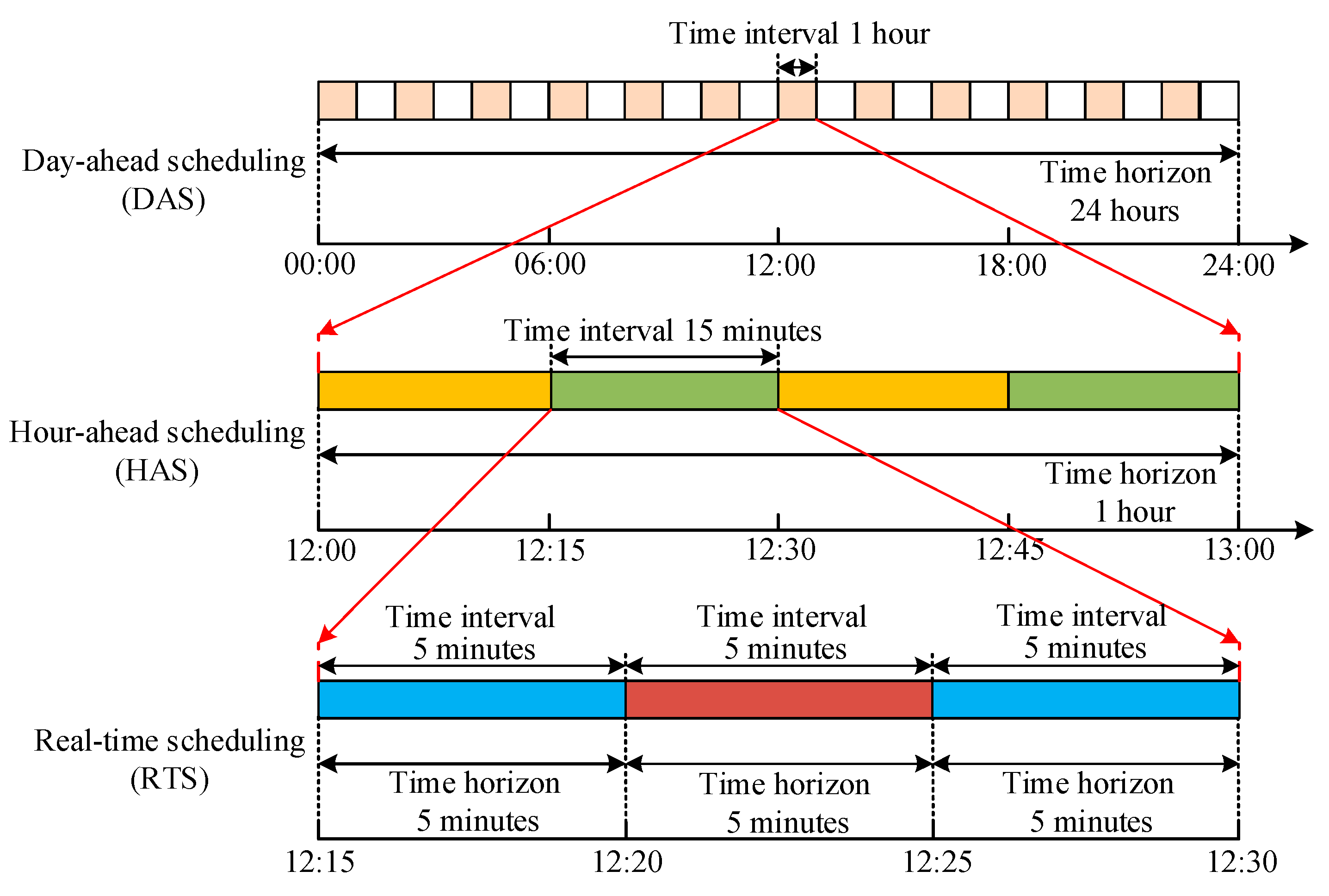
A hierarchical energy management framework incorporating the multi-timescale characteristics of the BES and DR along with the security constraints is proposed for an MG in grid-connected mode, which consists of DAS, hour-ahead scheduling (HAS), as well as real-time scheduling (RTS).
(2)
A decomposition-based algorithm is adopted to effectively settle the optimization models in the DAS and HAS.
(3)
Impacts of the multi-timescale characteristics of the BES and DR on the energy management of MG are analyzed.
The remainder of this paper is organized as follows. Section 2 describes the architecture of the hierarchical energy management. Section 3 presents the model formulation. Section 4 elaborates the solution algorithm. Section 5 demonstrates the simulation results. The conclusion is drawn in Section 6.

2. Architecture of the Hierarchical Energy Management

For the sake of clear description, the resources of MG in this paper will be stated first, and then the composition of the architecture elaborated. The sources of MG include the RES and dispatchable resources. Wind power (WD) is solely chosen to represent RES for its extensive application. The dispatchable resources comprise controllable distributed generation (CDG), BES, and DR. The CDG includes diesel engines (DE), the micro turbine (MT), and the fuel cell (FC). In view of the relatively high energy density, the all-vanadium redox flow battery is chosen as the BES [27]. Furthermore, DR programs are usually divided into two types: price-based DR and incentive-based DR [28]. The former can refer to customers’ autonomous response toward retail prices, while the latter would involve the active load change because of contract-based payments. Note that, the price-based DR is generally taken as non-controllable. The incentive-based DR could be considered as controllable since penalties would be enforced to customers who do not respond as required. As a result, the incentive-based DR is chosen as the DR program, and the interruptible power program is selected to represent the incentive-based DR for its popularization in this paper. In addition, the DRA is introduced to aggregate MG customers with small available interruptible power, and to make DR contracts with the MG operator [29]. The MG operator rewards the customers participating in DR contracts by two forms of payments, viz., capacity payment and energy payment [14]. If a certain amount of interruptible power is scheduled in DAS, the DRA will receive a capacity payment. If the interruptible power is further deployed in the operating day, the DRA will be rewarded an additional energy payment. Generally speaking, the unit energy payment of the deployed interruptible power is in inverse proportional to the time of advanced notice. Shorter advanced notice time could cause a larger effect on operation process, and thus lead to a larger unit energy payment [30].
The forecast accuracy of the output power of RES can increase with the reduction of prediction length. Meanwhile, the output power of RES usually fluctuates severely within an hour. In this context, the DAS with one-hour interval fails to utilize the intra-day forecast power of RES with higher precision, and cannot capture such fluctuation characteristics. In addition, the DAS cannot explore the multi-timescale characteristics of the BES and DR. Therefore, a hierarchical energy management framework is put forward. The framework comprises three stages of scheduling: DAS, HAS, and RTS. The relation among such scheduling is shown in Figure 1.
The DAS is conducted every 24 h with the temporal resolution of 1 h. The operation status of CDG, the charging and discharging power of BES, the exchanged power with the upstream grid, the scheduled interruptible power of DRA, together with the interruptible power deployed in DAS of DRA can be determined. Such variables will be taken as the input parameters of the HAS. The HAS is performed every hour with 15-min intervals. In this phase, the power of CDG and the interruptible power deployed in HAS of DRA can be decided. Meanwhile, the charging and discharging power of BES and the exchanged power with the upstream grid would be adjusted according to the forecast data of RES and the load within the next hour. The RTS is executed every 5 min for eliminating the imbalanced power because of the fluctuations of RES and load, by adjusting the operation of CDG and BES together with the exchanged power with the upstream grid. Additionally, the interruptible power deployed in RTS can also be used to realize the power balance.

3. Model Formulation

In this section, the optimization models of DAS and HAS as well as the control strategy of RTS will be discussed as follows. The notations used in the formulation are described in Table A1 (See Appendix A).

3.1. Day-Ahead Scheduling

To handle the uncertainty of RES and load, a scenario-based stochastic optimization model is formulated to optimize MG operation. Considering that the time interval of DAS is set to 1 h, the time interval is omitted to simplify the statement.

3.1.1. Objective Function

The objective in DAS is to minimize the expected operational cost of MG over the next 24 h. The cost comprises the cost of the exchanged power with the upstream grid, the startup/shutdown cost of CDG, the operation and maintenance cost (OMC) of BES, the capacity cost and day-ahead energy cost of DRA, the expected fuel cost and expected OMC of CDG, as well as the expected OMC of WD. Besides, although the RES in this model only includes WD, the model could be easily extended to the one with WD, solar power, and other RES.
min t = 1 T da [ c tu , t P tie , t + i = 1 N g ( c su , g , i Y g , i , t + c sd , g , i Z g , i , t ) + j = 1 N ba c om , ba , j ( P ba , j , t dis + P ba , j , t cha ) + k = 1 N dra ( c dra , k , t ca S P dra , k , t + c dra , k , t da , en D P dra , k , t da ) ] + s = 1 N s da ρ s t = 1 T da [ i = 1 N g ( C g , i , s , t fu + C g , i , s , t om ) + c om , wd P wd , s , t ]
C g , i , s , t fu = U g , i , t [ a g , i ( P g , i , s , t ) 2 + b g , i P g , i , s , t + c g , i ]
C g , i , s , t om = c om , g , i P g , i , s , t

3.1.2. Decision Variables

The involved decision variables in the DAS model are described as follows. Note that, the power of WD will be considered as the negative load instead of the decision variable, for the environment-friendly purpose.
X da = [ U g , i , t , Y g , i , t , Z g , i , t , P g , i , s , t , R g , i , s , t , U ba , j , t dis , P ba , j , t dis , U ba , j , t cha , P ba , j , t cha , R ba , j , s , t , U dra , k , t , S P dra , k , t , D P dra , k , t da , P tie , t ]
where i [ 1 , N g ] , j [ 1 , N ba ] , k [ 1 , N dra ] , s [ 1 , N s ] , t [ 1 , T da ] .

3.1.3. Constraints

1. System Constraints
For any time interval, the generated power in MG plus the exchanged power with the main grid should equal the sum of the load and network loss in (5). To reduce the influences of MG on the upstream grid, the spinning reserve is only provided by CDG, BES, and DRA in (6). Note that, the spinning reserve of DRA is identified as the scheduled interruptible power that is not deployed in DAS.
P tie , t + i = 1 N g P g , i , s , t + j = 1 N ba ( P ba , j , t dis P ba , j , t cha ) + k = 1 N dra D P dra , k , t da + P wd , s , t = P ld , s , t + P ls , s , t
i = 1 N g R g , i , s , t + j = 1 N ba R ba , j , s , t + k = 1 N la ( S P dra , k , t D P dra , k , t da ) R u 10
2. CDG Constraints
For each CDG, the output power is constrained by the maximum and minimum limits in (7). Constraint (8) represents the CDG’s ramp limits. The relations among the operation status, startup status, and shutdown status are described as (9). Constraints (10) and (11) enforce the minimum on and off time constraints, respectively. Constraint (12) defines the spinning reserve that can be supplied by CDG.
P g , i , min U g , i , t P g , i , s , t P g , i , max U g , i , t
r rd , g , i P g , i , s , t P g , i , s , t 1 r ru , g , i
{ Y g , i , t Z g , i , t = U g , i , t U g , i , t 1 Y g , i , t + Z g , i , t 1
{ h = 1 G g , i ( 1 U g , i , h ) = 0 h = t t + U T g , i 1 U g , i , h U T g , i Y g , i , t t = G g , i + 1 , , T da U T g , i + 1 h = t T da ( U g , i , h Y g , i , t ) 0 t = T da U T g , i + 2 , , T da
{ h = 1 H g , i U g , i , h = 0 h = t t + D T g , i 1 ( 1 U g , i , h ) D T g , i Z g , i , t t = H g , i + 1 , , T da D T g , i + 1 h = t T da ( 1 U g , i , h Z g , i , t ) 0 t = T D T g , i + 2 , , T da
0 R g , i , s , t min { U g , i , t r ru , g , i T 10 , P g , i , max P g , i , s , t , P g , i , s , t 1 + r ru , g , i P g , i , s , t }
3. BES Constraints
For each BES, the discharging and charging power are limited by the corresponding maximum and minimum limits in (13) and (14), respectively. Constraint (15) indicates that the charging and the discharging status of BES are mutually exclusive. The variation characteristics of the state of charge (SOC) of BES are defined in (16). Constraint (17) requires the SOC to be within the permissible range. In order not to affect BES operation in the next day, the SOC of BES at the end of the day is forced to be not less than a specific SOC limit in (18).
The model assumes that the BES can switch between the charging and discharging statuses in a short interval. Thus, the reserve supplied by the BES can be twice its rated power, theoretically [31]. Constraint (19) defines the reserve range of BES, which is restricted by both the rated power and the SOC limit.
0 P ba , j , t dis U ba , j , t dis P ba , j , max
0 P ba , j , t cha U ba , j , t cha P ba , j , max
0 U ba , j , t dis + U ba , j , t cha 1
S O C ba , j , t = S O C ba , j , t 1 + P ba , j , t cha η ba , j cha / E ba , j , max P ba , j , t dis / ( η ba , j dis E ba , j , max )
S O C ba , j , min S O C ba , j , t S O C ba , j , max
S O C ba , j , T da S O C ba , j lim
0 R ba , j , s , t min { E ba , j , max ( S O C ba , j , t S O C ba , j , min ) η ba , j dis / T 10 , P ba , j , max P ba , j , t dis + P ba , j , t cha }
4. DRA Constraints
For each DRA, the scheduled interruptible power is restricted by the maximum and minimum limits in (20). Considering customer satisfaction, the total response time of DRA is enforced to be not larger than a specific response time limit in (21). In the meantime, constraint (22) requires that the interruptible power is only allowed to be scheduled in the allowable time set. In (23), the interruptible power deployed in DAS cannot exceed the scheduled interruptible power.
U dra , k , t S P dra , k , t , min S P dra , k , t U dra , k , t S P dra , k , t , max
t = 1 T da U dra , k , t T dra , k lim
U dra , k , t = { 0 or 1 t ψ dra , k 0 else
0 D P dra , k , t da S P dra , k , t
5. Exchanged Power Constraints
The exchanged power is subject to the transmission capacity limit, whose positive or negative value represents the imported/exported power from/to the main grid.
P tie , max P tie , t P tie , max
6. Security Constraints
Constraint (25) represents the limits of power flow through each branch. Also, Constraint (26) requires the voltage at each bus should be within the allowable region.
S x , max S x , s , t S x , max
V y , min V y , s , t V y , max
where x [ 1 , N br ] , y [ 1 , N bs ] .

3.2. Hour-Ahead Scheduling

Based on the updated forecast data of RES and load, a deterministic optimization model is established in HAS to bridge the DAS and RTS. The decision variables of the DAS, stated in Section 3.1.2, would be regarded as the input parameters of HAS. Taking an example of the t-th HAS, the scheduling model is illustrated as below. Notice that, (t, m) indicates the m-th 15-min time interval at hour t.

3.2.1. Objective Function

The objective of MG operator in HAS is to minimize the operational cost in the following hour. The cost comprises the fuel cost and the OMC of CDG, the cost of the exchanged power with the upstream grid, the OMC of BES, the hour-ahead energy cost of DRA, and the OMC of WD. Besides, the penalty costs are added to follow the schedules of the DAS.
The fuel cost and the OMC of CDG are expressed as (28) and (29), respectively. Note that, U g , i , t is a known parameter which has been determined in the DAS.
min m = 1 N ha { i = 1 N g ( C g , i , t , m fu + C g , i , t , m om ) + { c tu , t P tie , t , m + j = 1 N ba c om , ba , j ( P ba , j , t , m dis + P ba , j , t , m cha ) + k = 1 N dra c dra , k , t ha , en P dra , k , t , m ha + c om , wd P wd , t , m + c pel , t | P tie , t P tie , t , m | + j = 1 N ba c pel , t | P ba , j , t dis P ba , j , t cha P ba , j , t , m dis + P ba , j , t , m cha | } / N ha }
C g , i , t , m fu = { [ a g , i ( P g , i , t , m ) 2 + b g , i P g , i , t , m + c g , i ] / N ha ( U g , i , t = 1 ) 0 ( U g , i , t = 0 )
C g , i , t , m om = c om , g , i P g , i , t , m / N ha
where | | is the absolute value function.

3.2.2. Decision Variables

The interruptible power deployed in HAS of DRA indicates the interruptible power which is not deployed in DAS, but deployed in HAS.
X ha = [ P g , i , t , m , R g , i , t , m , U ba , j , t , m dis , P ba , j , t , m dis , U ba , j , t , m cha , P ba , j , t , m cha , R ba , j , t , m , D P dra , k , t , m ha , P tie , t , m ]
where i [ 1 , N g ] , j [ 1 , N ba ] , k [ 1 , N dra ] , t [ 1 , N ha ] .

3.2.3. Constraints

1. System Constraints
The power balance constraint and the reserve constraint are described as (31) and (32), respectively. In (31), the interruptible power provided by DRA contains two parts. One is the interruptible power deployed in DAS, and the other is the interruptible power deployed in HAS. In (32), the spinning reserve of DRA corresponds to the interruptible power that has been scheduled, but not deployed in both the DAS and HAS.
P tie , t , m + i = 1 N g P g , i , t , m + j = 1 N ba ( P ba , j , t , m dis P ba , j , t , m cha ) + P w d , t , m + k = 1 N dra ( D P dra , k , t da + D P dra , k , t , m ha ) = P ld , t , m + P ls , t , m
i = 1 N g R g , i , t , m + j = 1 N ba R ba , j , t , m + k = 1 N dra [ S P dra , k , t ( D P dra , k , t da + D P dra , k , t , m ha ) ] R u 10
2. CDG Constraints
Given that the operation states of CDG have been yielded in DAS, the CDG constraints only comprise the power limit constraint, the ramp constraint, and the reserve constraint, which are similar to the Constraints (7), (8), and (12), respectively. Note that, such constraints need to be modified by replacing the subscript (t) with (t, m). Furthermore, additional constraints on the power and the reserve of CDG in the last 15-min time interval are imposed due to the decided operation state and the ramp limit, which are as follows.
P g , i , t , N ha r rd , g , i Z g , i , t + 1 / N ha + ( 1 Z g , i , t + 1 ) P g , i , max
R g , i , t , N ha r r d , g , i Z g , i , t + 1 / N ha + ( 1 Z g , i , t + 1 ) P g , i , max P g , i , t , N ha
In (33) and (34), the power and the reserve of CDG in the last 15-min time interval would be restricted by the operation state of CDG at hour (t + 1).
3. BES Constraints
The BES constraints comprise the charging power limit constraint, the discharging power limit constraint, the mutual exclusion constraint of charging and discharging states, the SOC limit constraint, and the reserve constraint, which are similar to the constraints (13)–(17), and (20), respectively. Note that, since the time horizon of HAS is 1 h, the constraint on the SOC of BES at the end of the day is not involved in this model.
4. DRA Constraints
For each DRA, the interruptible power deployed in HAS is subject to the following limits.
0 D P dra , k , t , m ha S P dra , k , t D P dra , k , t da
5. Exchanged Power Constraints and Security Constraints
The exchanged power constraints and security constraints are similar to those in the model of the DAS, which are not elaborated for space saving.

3.3. Real-Time Scheduling

There exist two steps in the control strategy of RTS. The first step is to calculate the initial power references of the CDG, BES, DRA, and exchanged power, on the basis of the results from the HAS. The second step is to adjust the power references to absorb the imbalanced power. Taking the interval (t, m, n) as the instance, the detailed steps are illustrated as below. Notice that, (t, m, n) represent the n-th 5-min time interval in the m-th 15-min time interval at hour t.

3.3.1. Calculate the Initial Power References

1. CDG
Considering the ramp limits, it will always consume a lot of time to vary from P g , i , t , m 1 to P g , i , t , m . Referring to [12], P g , i , t , m , n ini is assumed to change from P g , i , t , m 1 to P g , i , t , m at the maximum ramp rate first, and then stay at P g , i , t , m . Based on this, the initial power references of CDG are determined as in (36).
P g , i , t , m , n ini = { min { P g , i , t , m , n 1 fna + r ru , g , i / ( N ha N rl ) , P g , i , t , m } ( P g , i , t , m , n 1 fna P g , i , t , m ) max { P g , i , t , m , n 1 fna r ru , g , i / ( N ha N rl ) , P g , i , t , m } ( P g , i , t , m , n 1 fna > P g , i , t , m )
2. BES
In view of the SOC bounds, the initial power references of BES are decided as below. When the power reference is positive, it indicates the BES is in discharge state; vice versa, when the power reference is negative, it represents that BES can charge.
If P ba , j , t , m dis P ba , j , t , m cha 0
P ba , j , t , m , n ini = min { ( S O C ba , j , t , m , n 1 S O C ba , j , min ) E ba , j , max η ba , j dis N ha N rl , P ba , j , t , m dis P ba , j , t , m cha }
else
P ba , j , t , m , n ini = max { ( S O C ba , j , t , m , n 1 S O C ba , j , max ) E ba , j , max N ha N rl / η ba , j cha , P ba , j , t , m dis P ba , j , t , m cha }
end
3. DRA and Exchanged Power
Referring to the actual operation experiences, both the power of DRA and the exchanged power cannot be affected by the ramp constraints. Therefore, their initial power references are expressed as below.
D P dra , k , t , m , n ini = D P dra , k , t da + D P dra , k , t , m ha
P tie , t , m , n ini = P tie , t , m

3.3.2. Revise the Power References

For the uncertainties from RES and load, it is evitable to yield the imbalanced power. Moreover, the imbalanced power may also be aroused because of the ramp constraints of CDG and the SOC limits of BES. Thereby, the imbalanced power is given as follows.
Δ P t , m , n = P ld , t , m , n P wd , t , m , n i = 1 N g P g , i , t , m , n ini j = 1 N ba P ba , j , t , m , n ini k = 1 N dra D P dra , k , t , m , n ini P tie , t , m , n ini
To reduce the negative effects of MG on the upstream grid, the imbalanced power should be fully absorbed by the internal devices of MG if possible [9,10]. Since frequent power changes can jeopardize the working life of CDG and the comfort level DRA, CDG and DRA should avoid the frequent power response. Hence, the BES should accommodate the imbalanced power as far as possible. That is to say, the imbalanced power should be absorbed by the BES first, and then by CDG and DRA. The detailed instructions are presented as below.
1. Revise the Power References of BES
The imbalanced power could be distributed to the BES according to the proportion of the upward/downward regulation capacity in the total regulation capacity [32].
The upward/downward regulation capacities of a BES can indicate the maximal increment values of the discharging/charging power of the BES, respectively. The detailed formulations are given as follows.
{ P ba , j , t , m , n uc = min { ( S O C ba , j , t , m , n 1 S O C ba , j , min ) E ba , j , max η ba , j dis N ha N rl , P ba , j , max } P ba , j , t , m , n ini P ba , j , t , m , n dc = P ba , j , t , m , n ini max { ( S O C ba , j , t , m , n 1 S O C ba , j , max ) E ba , j , max N ha N rl / η ba , j cha , P ba , j , max }
Taking an example of the downward regulation capacity, it would equal the initial power reference minus the maximal charging power. The maximum charging power is limited by both the SOC limit and the rated power.
The upward and downward total regulation capacities are described as below.
{ P ba , t , m , n utc = j = 1 N ba P ba , j , t , m , n uc P ba , t , m , n dtc = j = 1 N ba P ba , j , t , m , n dc
The final power references of BES are expressed as below.
If Δ P t , m , n 0
P ba , j , t , m , n fna = min { 1 , Δ P t , m , n / P ba , t , m , n utc } P ba , j , t , m , n uc + P ba , j , t , m , n ini
else
P ba , j , t , m , n fna = max { 1 , Δ P t , m , n / P ba , t , m , n dtc } P ba , j , t , m , n dc + P ba , j , t , m , n ini
end
Therefore, the updated imbalanced power is described as follows.
Δ P t , m , n Δ P t , m , n j = 1 N ba ( P ba , j , t , m , n fna P ba , j , t , m , n ini )
where is the assigning operator.
2. Revise the Power References of CDG and DRA
When the imbalanced power is nonzero, the CDG and DRA will be utilized to further absorb the remaining imbalanced power successively. The detailed calling sequence depends on the CDG’s and DRA’s unit costs per kWh [33]. The CDG can accommodate the imbalanced power by increasing or decreasing their output power. However, to minimize the disturbance to the production and life of customers in the DRA, the DRA is only used to accommodate the imbalanced power through deploying the new interruptible power within the range of the scheduled interruptible power. Note that the unit energy cost of the interruptible power deployed in RTS is larger than that of the interruptible power deployed in DAS and HAS, owing to the shorter advanced notice time. Then, the residual imbalanced power will be totally accommodated by the main grid.
After the operation simulation during the whole day, the operation simulation cost of MG could be evaluated as follows.
C os = t = 1 T da [ i = 1 N g ( c su , g , i Y g , i , t + c sd , g , i Z g , i , t ) + k = 1 N dra c dra , k , t ca S P dra , k , t ] + t = 1 T da m = 1 N ha n = 1 N rl { i = 1 N g ( C g , i , t , m , n fu + C g , i , t , m , n om ) + { c tu , t P tie , t , m , n fna + j = 1 N ba c om , ba , j | P ba , j , t , m , n fna | + k = 1 N dra [ c dra , k , t da , en D P dra , k , t da + c dra , k , t ha , en D P dra , k , t , m ha + c dra , k , t rl , en ( D P dra , k , t , m , n fna D P dra , k , t da D P dra , k , t , m ha ) + c om , wd P wd , t , m , n } / ( N ha N rl ) }

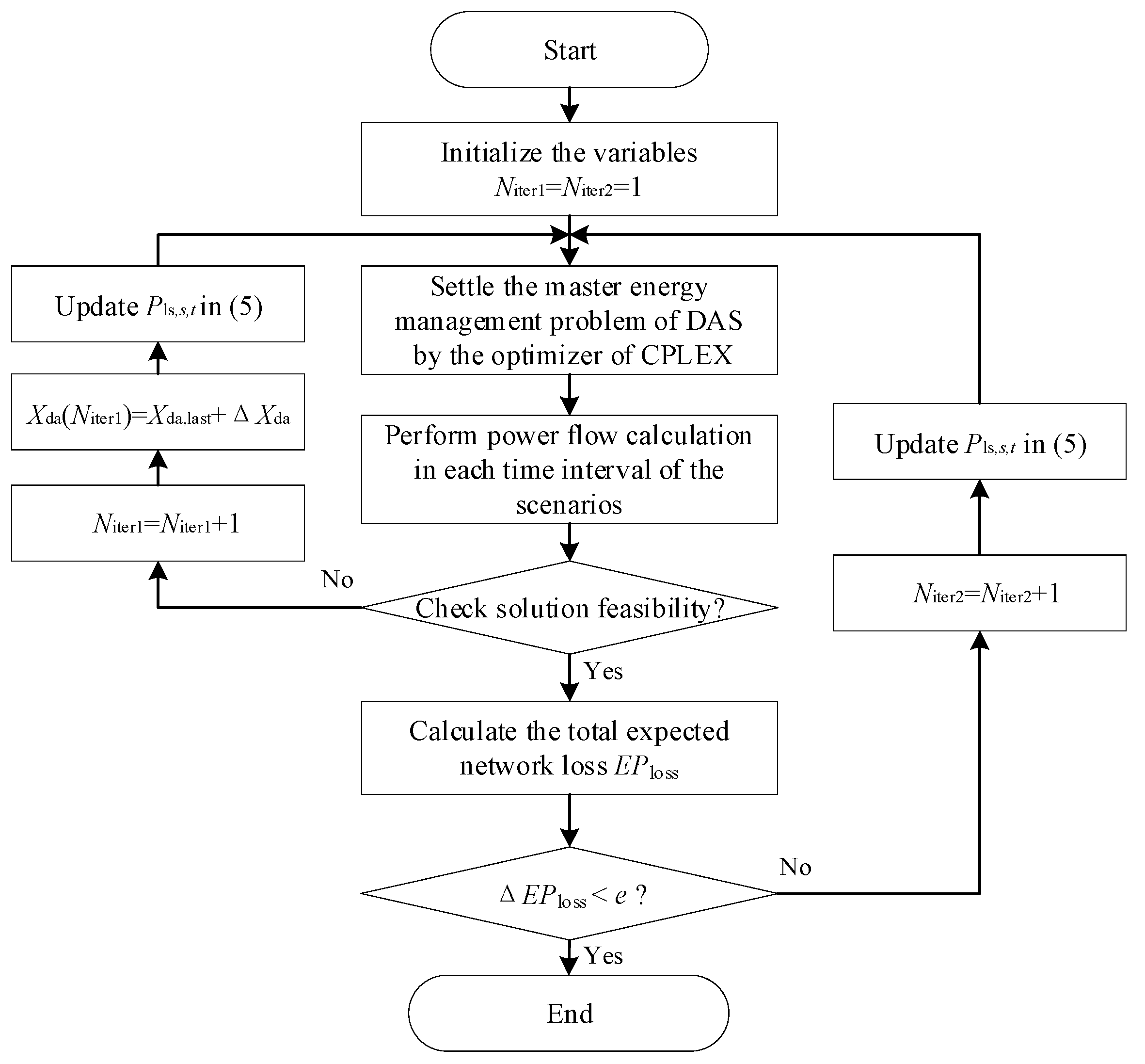
4. Solution Algorithm

In the hierarchical management framework, the optimization models of the DAS and HAS are both mixed-integer nonlinear programming (MINLP) problems, which are solved by a decomposition-based algorithm. The control strategy of the RTS can be implemented by a heuristic algorithm.
The MINLP problems are broken down into a master problem and an auxiliary problem. Taking the DAS as an example, the master problem is to settle the energy management problem (1)–(24), excluding the security Constraints (25) and (26). The auxiliary problem is to calculate the power flow based on the scheduling results from the master problem. Then in each time interval, both the power flow through each branch and the voltage of each bus will be checked to see whether they exceed the limits. The master problem and the auxiliary problem are implemented iteratively until the change of the total expected network loss is not larger than the tolerance limit e. The decomposition-based algorithm contains two critical steps. The first is to transform the master problem into a mixed-integer linear programming (MILP) problem. The second is to solve the master problem and the auxiliary problem iteratively.
In the optimization model of the DAS, the nonlinearity of the master problem is derived from the quadratic cost function of CDG. Therefore, piecewise linear approximation is introduced to linearize the quadratic cost function [34]. With regard to the optimization model of the HAS, besides the fuel cost of CDG, the penalty cost is another factor leading to the nonlinearity of the master problem. Here, the auxiliary variables and additional constraints can be employed to linearize such a penalty cost [12]. Based on these, the master energy scheduling problems of the DAS and HAS are both converted to MILP problems.
The iterative solution is the core of the decomposition-based algorithm. Taking the DAS as an example, the flowchart of the iterative solution is depicted in Figure 2. Notice that, Niter1 and Niter2 are both the counters of the algorithm.
(1)
The linearized master energy management problem is solved by the optimizer of CPLEX, and then the scheduling results Xda will be obtained.
(2)
The power flow calculation is implemented in each time interval of scenarios, and the security constraints would be checked to see whether they are met.
(3)
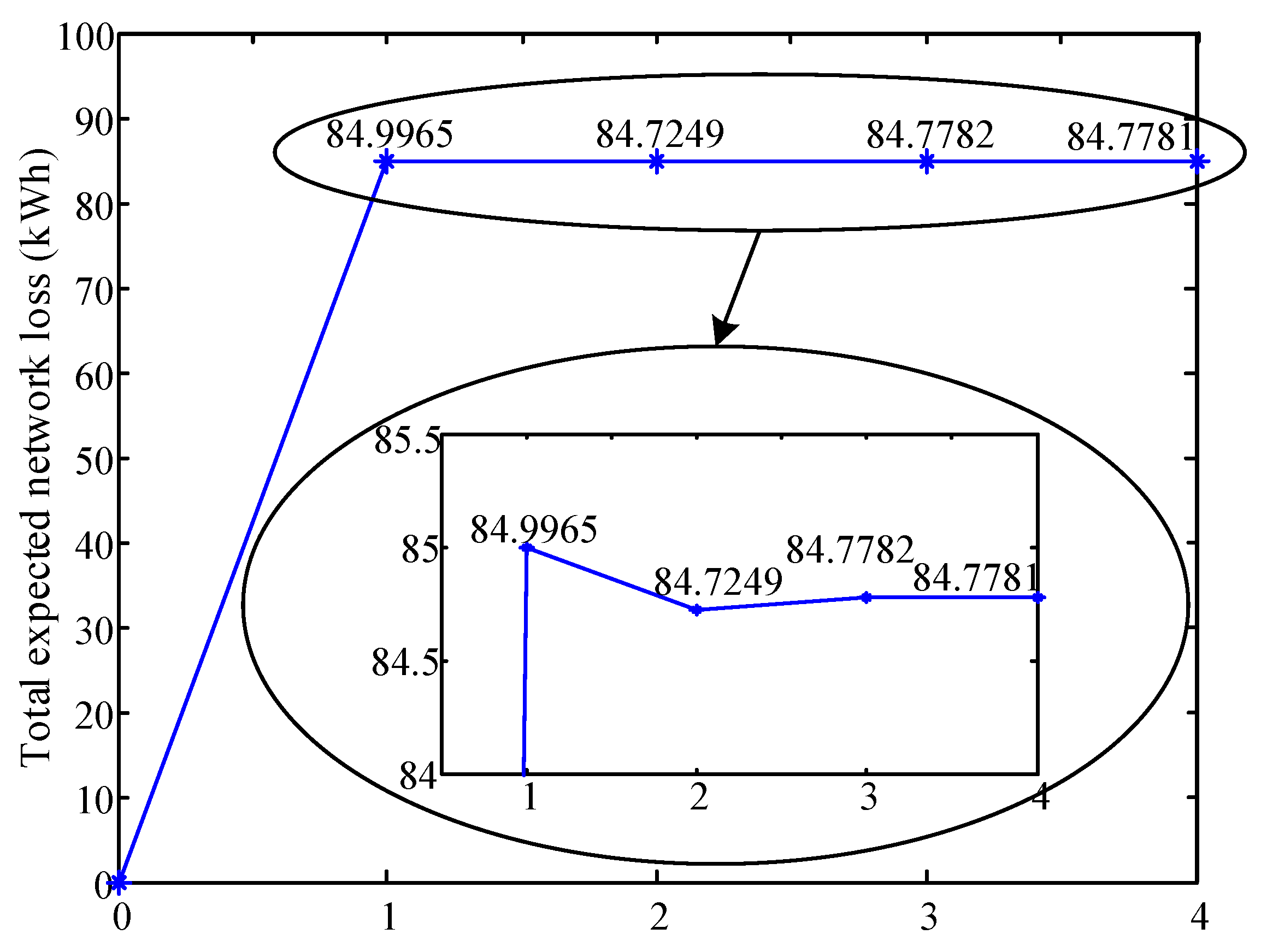
When there exists a violation of security constraints, a tiny random vector ΔXda will be added to the last feasible solution Xda,last to calculate the power losses again. Then, the master problem will be rerun using the updated power balance constraints (5). [2]. If there is no violation of the constraints, the power loss will be calculated in each time interval of the scenarios, and the total expected network loss EPloss would be decided. The newly calculated power losses will be returned to the master problem for updating the power balance constraints (5), until the variation of the total expected network loss ΔEPloss is less than the tolerance limit e.
(4)
After finite iterations, a new steady-state condition can be determined.
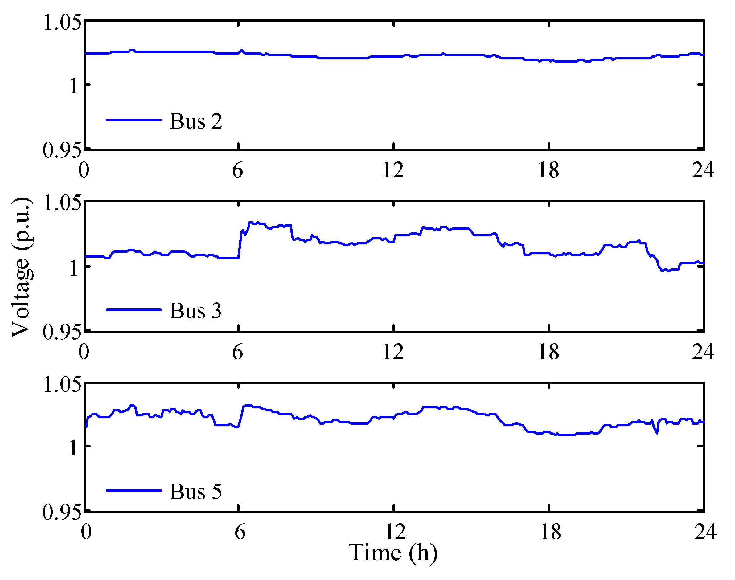
The flowchart of the iterative solution for the HAS is similar to that for the DAS, which is not expressed for space saving.

5. Case Study

An MG system is shown in Figure 3, whose network parameters can be obtained from [12]. The MG consists of a DE, an MT, an FC, a wind turbine, a BES, and a DRA. The technical and economic parameters of CDG and RES are summarized in Table 1. For BES, its rated power and capacity are 50 kW and 200 kWh, respectively. The charging efficiency and discharging efficiency are both set to 0.922. The maximum allowable SOC, initial SOC, minimum allowable SOC, and the SOC limit at the end of the day are set as 1, 0.5, 0.2, and 0.5, respectively. The unit OMC is 0.008 $/kWh. For DRA, the upper and lower limits of scheduled interruptible power are chosen as 80 kW and 30 kW, respectively. The response time limit is set as 12 h. The time set of allowing the interruptible power to be scheduled is [7:00, 22:00]. Furthermore, the maximum exchanged power with the main grid is 500 kW. The time-of-use price of a province in China is depicted in Figure 4. Referring to [25], the unit capacity cost of scheduled interruptible power for DRA is also depicted in Figure 4. To follow the operation results of DAS, it is assumed that the penalty cost is 1.5 times the time-of-use price. Also, the unit energy cost of the interruptible power deployed in DAS, HAS, and RTS are assumed to be five times, eight times, and 10 times the unit capacity cost of the scheduled interruptible power.
The scenarios in DAS can be generated according to the following procedure. First, we assume that the MG operator could acquire forecast data of RES and the load from a local forecast center. Moreover, considering that any forecast technique can suffer from forecast errors, we also assume that the MG operator can fit the forecast error data into suitable distributions. For simplicity, it is assumed that the forecast errors of WD and load follow normal distributions with zero-mean. Their standard deviations are set as 5% and 2% of their forecast values, respectively [35]. Based on this information, 10,000 scenarios with equal probability (1/10,000) are generated. To balance the computational burden and modeling accuracy, the fast-forward scenario reduction technique is used to reduce the original 10,000 scenarios to 10 scenarios [36]. Furthermore, since the power of WD and load for the next hour can be forecasted quite accurately [37,38], their forecast values will be directly regarded as the input data of WD and load for the deterministic model of HAS, to satisfy the requirement on solution speed. The imbalanced power mainly from the difference between the power of WD and load in HAS and that in RTS, would be absorbed by the components within the MG.
Figure 5 depicts the predicted values of WD and load in 24 h with 15-min interval. To test the effectiveness of the proposed hierarchical framework, the actual data with 5-min intervals are also shown in Figure 5. The simulation platform is Matlab 2013(a) on a PC with Intel Core dual i5-4220M (2.5 GHz) and 16 GB RAM.

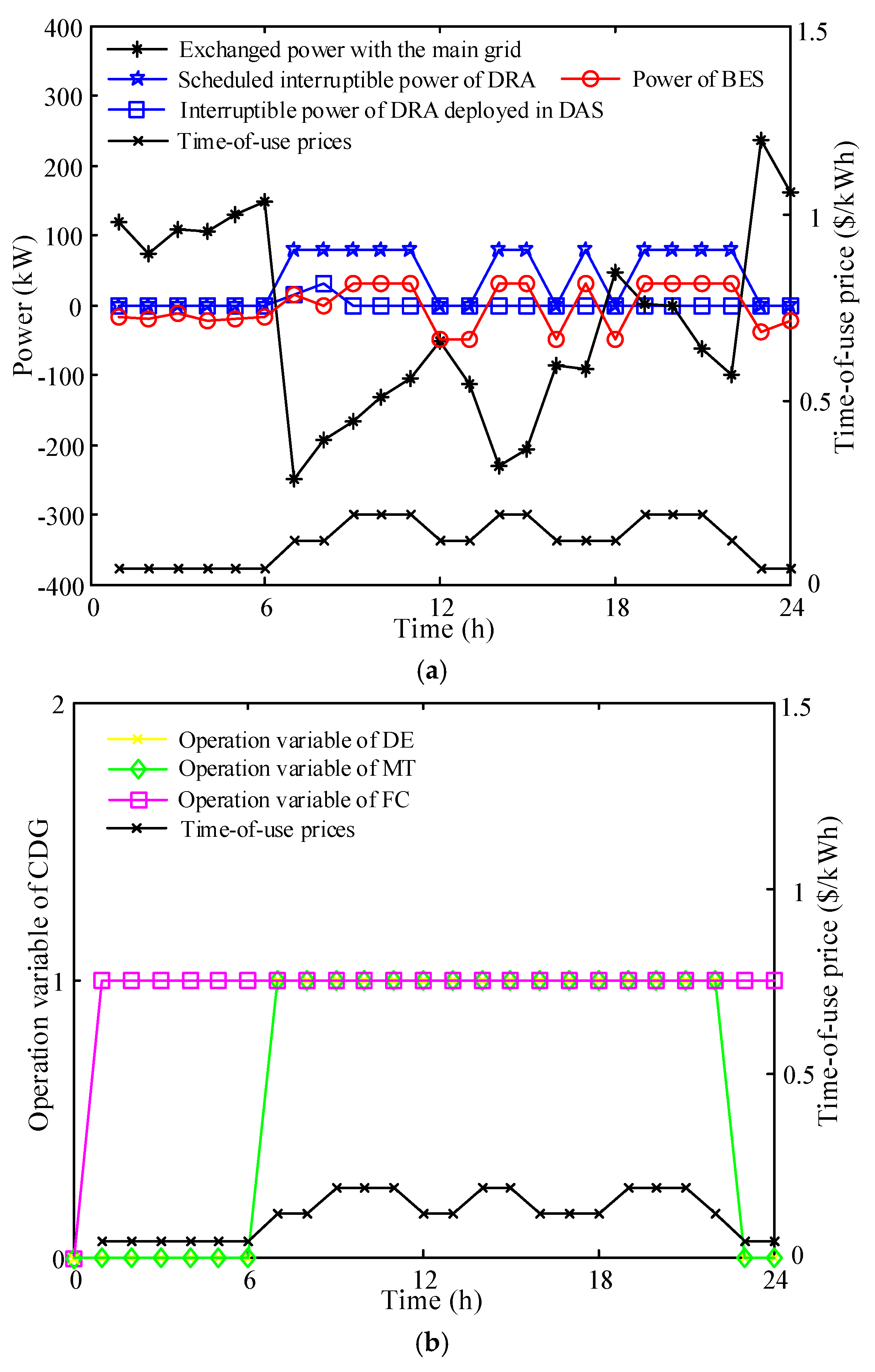
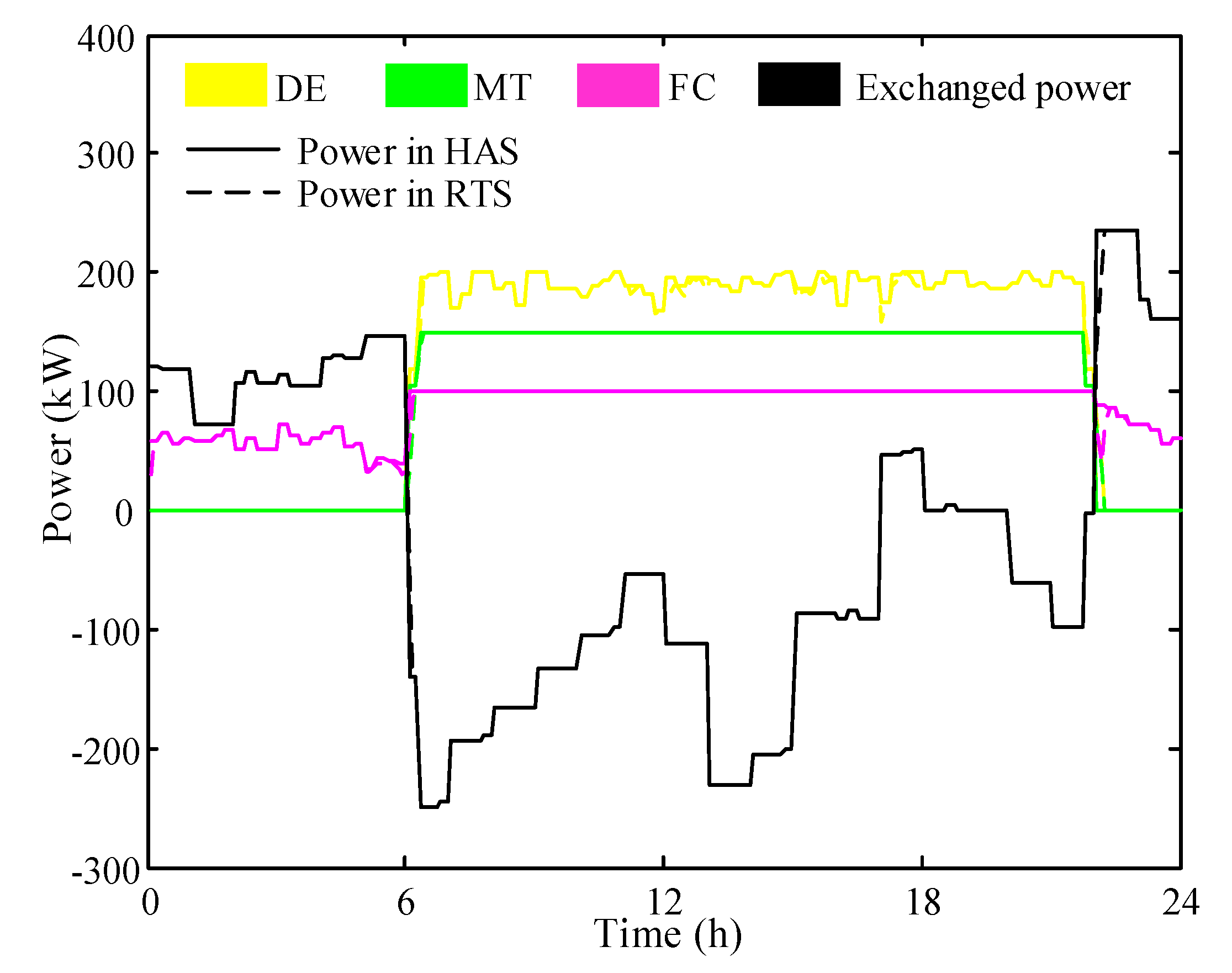
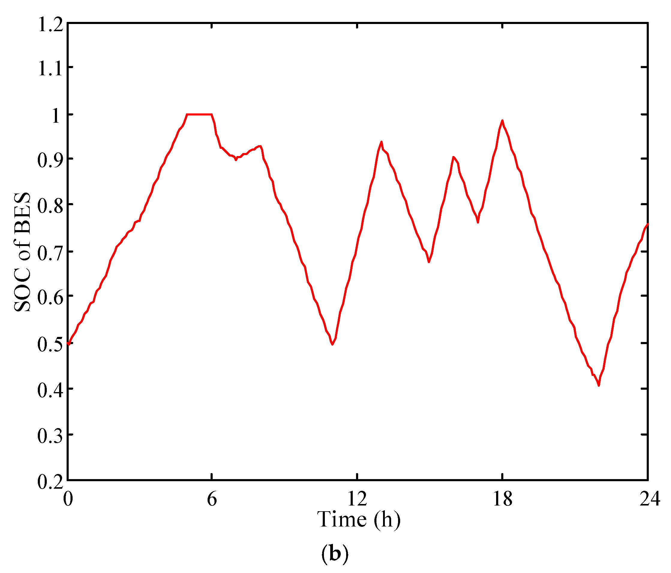
5.1. Simulation of the Hierarchichal Energy Management

To analyze the convergence characteristic of the decomposition-based algorithm, taking the DAS as an example, the total expected network loss of the MG at each iteration is shown in Figure 6. The number of iterations is four with the tolerance of this algorithm e being 10−4 kWh. Meanwhile, the calculation time is only 6.806 s. Specifically, it takes 2.148 s to solve the master problem, whereas it takes 4.658 s to implement the power flow subproblem. Since the calling cycle of DAS is 24 h, this computation speed is fast enough to meet the online operation demand of the DAS.
First, it is assumed that the total expected network loss is 0 kWh. Subsequently, the total expected network loss turns into 84.9965 kWh. The newly calculated power losses will be return to the master problem for updating the power balance constraints (5), if only the variation of the total expected network loss is not less than the tolerance limit. After four iterations, the system converges to a steady status where the optimum solutions can be determined.
The convergence procedure of solving the HAS is similar to that of solving the DAS. Among all the calling of HAS, the maximum iterations is five, and the largest solution time is 0.222 s. Since the calling cycle of HAS is 1 h, the computation speed can fully meet the online operation demand of HAS.
The algorithm can also be effective with larger test systems. Taking a revised IEEE 33-bus system as an example, the system consists of two DE, two MT, two FC, a wind turbine, a BES, and a DRA. For the DAS, the number of iterations is nine with e being 10−4 kWh. Meanwhile, the computation time is only 15.479 s. Similar results can be obtained for the HAS, which are not described for space saving.
The DAS is conducted first, and then part of the decision variables will be input to the HAS as known parameters. The decision variables that are passed to the HAS are depicted in Figure 7.
According to Figure 7, the MG inclines to import power from the upstream grid in low-price periods, and export power in high-price periods. Similarly, the BES would charge within low-price periods and discharge within high-price periods. Meanwhile, due to the cheap operation cost, the FC firstly starts up at hour 1, and then stays online for the remaining periods. On the contrary, both the DE and MT only start up at hour 7, then shut down at hour 23. For DRA, the interruptible power is often scheduled during high-price periods, but the interruptible power is only deployed at hours 7 and 8. Moreover, the deployed interruptible power is relatively low. This indicates that the scheduled interruptible power is mainly utilized to supply the reserve of MG instead of participating in the power balance, mostly because of the low unit capacity cost and the high unit energy cost.
Based on such decision variables, the HAS is then performed. After calling the HAS, the RTS would be implemented on a 5-min interval to accommodate the imbalanced power. Both the power of the CDG and the exchanged power in HAS and RTS are shown in Figure 8.
From Figure 8, the exchanged power in HAS can effectively follow the DAS plan. Since the energy efficiency of FC is the largest among all CDG, it is generally given the highest priority in daily operation. Meanwhile, after the startup of the DE and MT, the MT will operate almost at its rated power, whereas the power fluctuation of the DE is significant. This is because the DE is with the lowest energy efficiency, and is always arranged in the lowest priority. In addition, the deviations between the power in HAS and RTS for the CDG and exchanged power are extremely tiny. This can help increase the operation stability of CDG and improve the power quality of the upstream grid.
The power of the BES and DRA in HAS and RTS are both given in Figure 9a. Besides, the SOC of the BES in RTS is exhibited in Figure 9b.
As shown in Figure 9a, similar to the exchanged power, the power of BES in HAS can effectively follow the DAS plan due to the high penalty cost. Since the BES is first used to accommodate the imbalanced power in RTS, the power of BES in RTS would fluctuate around the referenced power determined by the HAS. Moreover, the interruptible power of DRA is not deployed in HAS, mainly due to the high unit energy cost in the HAS. Note that, although the unit energy cost in RTS is larger than that in HAS, the interruptible power is still deployed in RTS at the startup of the DE and MT. This can be explained by the fact that the CDG cannot fully follow the drastic variation of the exchanged power owing to its ramp limits, which thereby leads to a large imbalanced power. For the power limit of BES, the imbalanced power cannot be fully accommodated by the BES. In this context, the interruptible power of DRA has to be deployed to eliminate the remaining imbalanced power for decreasing the disturbance to the exchanged power.
According to Figure 9b, it can be observed that the SOC of BES can stay within the allowable range during the whole day, which ensures the secure operation of BES. Furthermore, we can also see that the SOC of BES at the end of the day is slightly larger than the initial SOC. This is mainly because, in this day, the actual power of WD in RTS is generally larger than the predicted power in HAS at the end of the day such as hours 23 and 24, shown in Figure 5. In this case, the charging power of BES at such hours has to be increased to accommodate the imbalanced power, further leading to the rise of SOC.
In addition, the load flow of all branches and the voltage of all buses across the whole time horizon are within the safe region. Figure 10 depicts the voltage variations of three typical buses (bus 2, bus 3, and bus 5) in the day.
It can be discovered from Figure 10 that the voltage of bus 2 stays around 1.025 p.u. due to the domination of the upstream grid. Bus 3 locates at the middle of the topology. As the DE starts up at hour 7, there exists a marked rise for the voltage of bus 3, whereas the voltage would decrease with the shutdown of the DE. Bus 5 locates at the terminal of the topology and is also linked with the FC. Although the voltage of bus 5 is a little high, it is still within the safe region, viz. 0.95–1.05 p.u. As a result, the produced operation resulting from the hierarchical energy management framework is safe.

5.2. Impacts of the Multi-Timescale Characteristics of the BES and DR on the Energy Management of MG

In order to analyze the impacts of the multi-timescale characteristics of BES and DR on the energy management of MG, four cases are described in Table 2. Each case represents an energy management method of MG. In case 1, the energy management method is exactly the proposed hierarchical energy scheduling framework in this paper. In case 2, the energy management method is similar to that in case 1. The only difference is that the multi-timescale characteristic of DR is not considered. The DRA is only involved in DAS, but is not involved in HAS and RTS. In other words, the scheduled interruptible power along with the interruptible power deployed in DAS of DRA will be decided according to the model in DAS. However, the interruptible power deployed in HAS and RTS are both zero. The method in case 3 is also similar to that in case 1. Nevertheless, the charging/discharging power of BES is determined in DAS, and will remain unchanged in HAS and RTS. The method in case 4 can be considered as a combination of the methods in cases 2 and 3, which is not described for space saving.
The operation simulation results of such cases are shown in Table 3. There are two comparison indexes: one is the frequency of power adjustment in RTS (FPAR), and the other is the accumulated adjusted power in RTS (AAPR). The former is the number of the time intervals of RTS, when the output power of a source in RTS is different from that in HAS. Meanwhile, the latter means the sum of the absolute value of the difference between the output power of a source in RTS and that in HAS. The operation stability of CDG would increase with the decline of the FPAR and AAPR, and the power quality of the main grid can be improved as the FPAR and AAPR decrease.
It can be observed from Table 3 that the involvement of the multi-timescale characteristics of BES and DR would contribute to the reduction of the FPAR and AAPR for the CDG and exchanged power. Besides, based on the results of cases 2, 3, and 4, the involvement of the multi-timescale characteristic of BES can be more effective to reduce the FPAR and AAPR, compared with that of DR. This is mainly because the capability of BES to accommodate the imbalanced power in RTS is significantly greater than that of DRA. Specifically, the BES can accommodate the imbalanced power by adjusting the charging/discharging power flexibility. However, to reduce the disturbance to the production and life of customers, the DRA is only utilized to accommodate the imbalanced power by deploying the new interruptible power. Moreover, for the high unit energy cost of the interruptible power deployed in RTS, the DRA is often the last component in MG to be adopted for absorbing the imbalanced power.

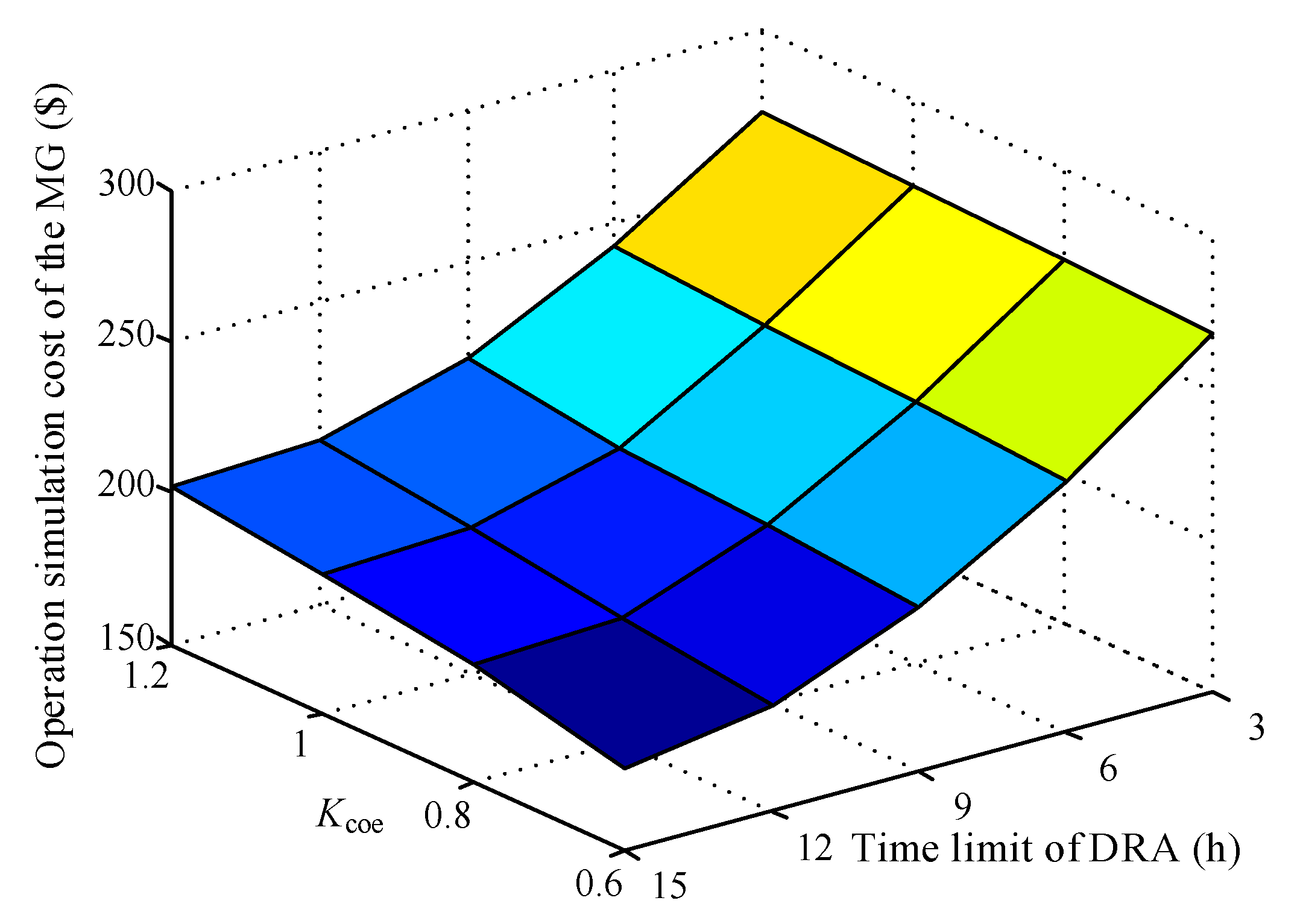
5.3. Impacts of the Cost and the Time Limit of DRA on the Energy Management of MG

Figure 11 illustrates the impacts of the cost and the time limit of DRA on the energy management of MG. For the convenience of analyzing, the ratios of the unit energy costs of the interruptible power deployed in DAS, HAS, and RTS to the unit capacity cost of the scheduled interruptible power are assumed to remain at 5, 8, and 10, respectively. Given this, the variation trends of such unit energy costs are determined by those of the unit capacity cost.
In this paper, the way of changing the unit capacity cost is as follows.
c dra , k , t ca = K coe c dra , k , t ca , ini
where c dra , k , t ca , ini is the initial unit capacity cost of scheduled interruptible power; K coe is the changing coefficient.
As seen from Figure 11, the operation simulation cost of MG can decrease with the reduction of the unit capacity cost of scheduled interruptible power under a certain time limit of DRA. Meanwhile, the operation simulation cost of MG will reduce with the increase of the time limit of DRA for a given unit capacity cost. This is because as the time limit rises, the interruptible power can be scheduled at more hours. In this context, the reserve burden of CDG can drop, and then the generation efficiency of CDG would increase. Therefore, the operation simulation cost of MG could show a decreasing tendency with the increase of the time limit.

6. Conclusions

A three-stage hierarchical energy management framework has been put forward to optimize MG operation under the uncertainty of RES and load, which takes account simultaneously of the multi-timescale characteristics of BES and DR together with the security constraints. The framework consists of DAS, HAS, and RTS. In DAS, a scenario-based stochastic optimization model is established to minimize the expected operational cost of MG, while ensuring its safe operation. In HAS, a deterministic model is presented to bridge DAS and RTS. In terms of the model characteristic, a decomposition-based algorithm is adopted to settle such models. In RTS, a control strategy is presented to eliminate the imbalanced power owing to the fluctuations of RES and load, under the premise of the minimal effects of the MG on the upstream grid.
Simulation results on a seven-bus MG demonstrate that the presented management framework can effectively yield an economic and safe scheduling plan. The adopted decomposition-based method can settle the models of DAS and HAS after several iterations. Meanwhile, the computation speed is fast enough to meet online operational requirements. In addition, the involvement of the multi-timescale characteristics of BES and DR in MG energy management would contribute to the improvement of the operation stability of CDG and the enhancement of the power quality of the upstream grid. Meanwhile, the involvement of the multi-timescale characteristic of BES can be more effective to reduce the FPAR and AAPR, compared with that of DR. Furthermore, the decreasing of the cost of DRA and the increasing of the time limit of DRA can both help reduce the operation simulation cost of MG.

Author Contributions

S.F. and Q.A. conceived and designed the research method; S.F. implemented the main research work and wrote the manuscript; and L.P. double-checked the proposed algorithm, the results, and the whole manuscript.

Funding

This research was funded by National Natural Science Foundation of China under Grant No. 51577115 and U1766207, and also by fund of China Scholarship Council (CSC).

Acknowledgments

This work is supported by National Natural Science Foundation of China (No. 51577115 and No. U1766207), and by fund of China Scholarship Council (CSC).

Conflicts of Interest

The authors declare no conflict of interest.

Appendix A. Notations for the Model Formulation

Table A1. Notations for the model formulation.
Acronyms
MGMicrogrid
WDWind power
BESBattery energy storage
DRADemand response aggregator
CDGControllable distributed generators
SOCState of charging
Parameters
N g , N ba , N dra Number of CDG, BES, and DRA
N bs , N br Number of buses and branches
T da Number of hours in a day
N s da Number of scenarios
ρ s Probability of scenario s
c om , g , i , c om , ba , j , c om , wd Unit OMC of CDG i, BES j, and WD
c tu , t Time-of-use price at hour t
c pel , t , Penalty price at hour t
R u 10 Required spinning reserve
S x , max Maximum thermal limit of branch x
V y , max , V y , min Maximum and minimum bounds of the voltage of bus y
c su , g , i , c sd , g , i Startup and shutdown costs
a g , i , b g , i , c g , i Coefficients of the quadratic cost function of CDG i
P g , i , max , P g , i , min Maximum and minimum operation limits of CDG i
r ru , g , i , r rd , g , i Ramp up and ramp down rates of CDG i
U T g , i , D T g , i Minimum on and off time of CDG i
G g , i , H g , i Required on and off time at the start time of the day of CDG i
T 10 Response time of the spinning reserve (e.g., 10 min)
P ba , j , max , E ba , j , max Maximum power and capacity of BES j
η ba , j cha , η ba , j dis Charging and discharging efficiency factors of BES j
S O C ba , j , max , S O C ba , j , min Maximum and minimum permissible SOC of BES j
S O C ba , j lim SOC limit at the end of the day of BES j
c dra , k , t ca 
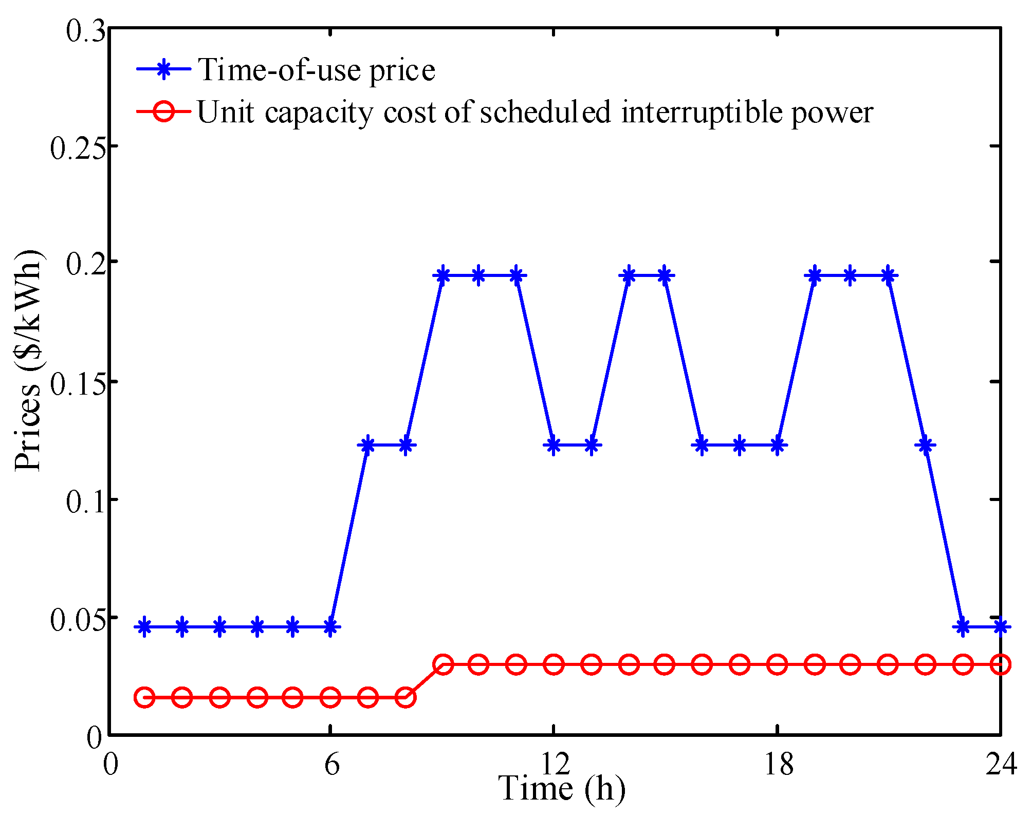
Unit capacity cost of the scheduled interruptible power of DRA k at hour t
c dra , k , t da , en , c dra , k , t ha , en , c dra , k , t rl , en Unit energy cost of the interruptible power deployed in DAS, HAS, and RTS of DRA k at hour t
S P dra , k , t , max , S P dra , k , t , min Maximum and minimum bounds of the scheduled interruptible power of DRA k at hour t
T dra , k lim Response time limit of DRA k
ψ dra , k Allowable time set of the scheduling interruptible power of DRA k
P tie , max Transmission capacity limit of the exchanged power
Variables
U g , i , t , Y g , i , t , Z g , i , t Operation status, startup status, and shutdown status of CDG i at hour t
P g , i , s , t , R g , i , s , t Power and spinning reserve of CDG i at hour t in scenario s
U ba , j , t dis , U ba , j , t cha Discharging and charging statuses of BES j at hour t
P ba , j , t dis , P ba , j , t cha Discharging and charging power of BES j at hour t
R ba , j , s , t Spinning reserve of BES j at hour t in scenario s
U dra , k , t Operation status of DRA k at hour t
S P dra , k , t Scheduled interruptible power of DRA k at hour t
D P dra , k , t da Interruptible power deployed in DAS of DRA k at hour t
P tie , t Exchanged power with the main grid at hour t
S x , s , t , V y , s , t Load flow of branch x and voltage of bus y at hour t in scenario s
P ld , s , t , P ls , s , t Load and network loss at hour t in scenario s
P wd , s , t Power of WD at hour t in scenario s
(t, m)The m-th 15-min time interval at hour t
P g , i , t , m , R g , i , t , m Power and spinning reserve of CDG i
U ba , j , t , m dis , U ba , j , t , m cha Discharging and charging statuses of BES j
P ba , j , t , m dis , P ba , j , t , m cha Discharging and charging power of BES j
R ba , j , t , m Spinning reserve of BES j
D P dra , k , t , m ha Interruptible power deployed in HAS of DRA k
P tie , t , m Exchanged power with the main grid
P ld , t , m , P ls , t , m Load and network loss
(t, m, n)The n-th 5-min time interval in the m-th 15-min time interval at hour t
Δ P t , m , n Imbalanced power of MG at real time
P g , i , t , m , n ini Initial power reference of CDG i
D P dra , k , t , m , n ini , D P dra , k , t , m , n fna Initial and final power references of DRA k
P ba , j , t , m , n ini , P ba , j , t , m , n fna Initial and final power references of BES j
P ba , j , t , m , n uc , P ba , j , t , m , n dc Upward and downward regulation capacities of BES j
P ba , t , m , n utc , P ba , t , m , n dtc Upward and downward total regulation capacities of BES j
P tie , t , m , n ini , P tie , t , m , n fna Initial and final power references of the exchanged power

References

  1. Fathima, A.H.; Palanisamy, K. Optimization in microgrids with hybrid energy systems—A review. Renew. Sustain. Energy Rev. 2015, 45, 431–446. [Google Scholar] [CrossRef]
  2. Su, W.; Wang, J.; Roh, J. Stochastic energy scheduling in microgrids with intermittent renewable energy resources. IEEE Trans. Smart Grid 2014, 5, 1876–1883. [Google Scholar] [CrossRef]
  3. Li, P.; Xu, D.; Zhou, Z.; Lee, W. Stochastic optimal operation of microgrid based on chaotic binary particle swarm optimization. IEEE Trans. Smart Grid 2016, 7, 66–73. [Google Scholar] [CrossRef]
  4. Ding, Z.; Lee, W. A stochastic microgrid operation scheme to balance between system reliability and greenhouse gas emission. IEEE Trans. Ind. Appl. 2016, 52, 1157–1166. [Google Scholar]
  5. Tavakoli, M.; Shokridehaki, F.; Akorede, M.F.; Marzband, M.; Vechiu, I.; Pouresmaeil, E. CVaR-based energy management scheme for optimal resilience and operational cost in commercial building microgrids. Int. J. Electr. Power Energy Syst. 2018, 100, 1–9. [Google Scholar] [CrossRef]
  6. Xiong, H.; Xiang, T.; Chen, H.; Lin, F.; Su, J. Research of fuzzy chance constrained unit commitment containing large-scale intermittent power. Proc. CSEE 2013, 33, 36–44. [Google Scholar]
  7. Xiang, Y.; Liu, J.; Liu, Y. Robust energy management of microgrid with uncertain renewable generation and load. IEEE Trans. Smart Grid 2016, 7, 1034–1043. [Google Scholar] [CrossRef]
  8. Wang, S.; Wang, D.; Han, L. Interval linear programming method for day-ahead optimal economic dispatching of microgrid considering uncertainty. Autom. Electr. Power Syst. 2014, 38, 5–11. [Google Scholar]
  9. Wu, X.; Wang, X.; Qu, C. A hierarchical framework for generation scheduling of microgrids. IEEE Trans. Power Deliv. 2014, 29, 2448–2457. [Google Scholar] [CrossRef]
  10. Bao, Z.; Zhou, Q.; Yang, Z.; Yang, Q.; Xu, L.; Wu, T. A multi time-scale and multi energy-type coordinated microgrid scheduling solution-Part I: Model and methodology. IEEE Trans. Power Syst. 2015, 30, 2257–2266. [Google Scholar] [CrossRef]
  11. Xu, X.; Jia, H.; Wang, D.; Yu, D.C.; Chiang, H. Hierarchical energy management system for multi-source multi-product microgrids. Renew. Energy 2015, 78, 621–630. [Google Scholar] [CrossRef]
  12. Xu, G.; Shang, C.; Fan, S.; Hu, X.; Cheng, H. A hierarchical energy scheduling framework of microgrids with hybrid energy storage systems. IEEE Access 2017, 6, 2472–2483. [Google Scholar] [CrossRef]
  13. Nolan, S.; O’Malley, M. Challenges and barriers to demand response deployment and evaluation. Appl. Energy 2015, 152, 1–10. [Google Scholar] [CrossRef]
  14. Sahin, C.; Shahidehpour, M.; Erkmen, I. Allocation of hourly reserve versus demand response for security-constrained scheduling of stochastic wind energy. IEEE Trans. Sustain. Energy 2013, 4, 219–228. [Google Scholar] [CrossRef]
  15. Talari, S.; Yazdaninejad, M.; Haghifam, M. Stochastic-based scheduling of the microgrid operation including wind turbines, photovoltaic cells, energy storages and responsive loads. IET Gener. Transm. Distrib. 2015, 9, 1498–1509. [Google Scholar] [CrossRef]
  16. Nguyen, D.T.; Le, L.B. Risk-constrained profit maximization for microgrid aggregators with demand response. IEEE Trans. Smart Grid 2015, 6, 135–146. [Google Scholar] [CrossRef]
  17. Nunna, H.S.; Doolla, S. Energy management in microgrids using demand response and distributed storage—A multiagent approach. IEEE Trans. Power Deliv. 2013, 28, 939–947. [Google Scholar] [CrossRef]
  18. Mehdizadeh, A.; Taghizadegan, N.; Salehi, J. Risk-based energy management of renewable-based microgrid using information gap decision theory in the presence of peak load management. Appl. Energy 2018, 211, 617–630. [Google Scholar] [CrossRef]
  19. Bui, V.; Hussain, A.; Kim, H. A multiagent-based hierarchical energy management strategy for multi-microgirds considering adjustable power and demand response. IEEE Trans. Smart Grid 2018, 9, 1323–1333. [Google Scholar] [CrossRef]
  20. Marzband, M.; Fouladfar, M.H.; Akorede, M.F.; Lightbody, G.; Pouresmaeil, E. Framework for smart transactive energy in home-microgrids considering coalition formation and demand side management. Sustain. Cities Soc. 2018, 40, 136–154. [Google Scholar] [CrossRef]
  21. Marzband, M.; Azarinejadian, F.; Savaghebi, M.; Pouresmaeil, E.; Guerrero, J.M.; Lightbody, G. Smart transactive energy framework in grid-connected multiple home microgrids under independent and coalition operations. Renew. Energy 2018, 126, 95–106. [Google Scholar] [CrossRef]
  22. Mohsenian-Rad, A.; Wong, V.; Jatskevich, J.; Schober, R.; Leon-Garcia, A. Autonomous demand-side management based on game-theoretic energy consumption scheduling for the future smart grid. IEEE Trans. Smart Grid 2010, 1, 320–331. [Google Scholar] [CrossRef]
  23. Maharjan, S.; Zhu, Q.; Zhang, Y.; Gjessing, S.; Basar, T. Demand response management in the smart grid in a large population regime. IEEE Trans. Smart Grid 2016, 7, 189–199. [Google Scholar] [CrossRef]
  24. Pourmousavi, S.A.; Nehrir, M.H.; Sharma, R.K. Multi-timescale power management for islanded microgrids including storage and demand response. IEEE Trans. Smart Grid 2015, 6, 1185–1195. [Google Scholar] [CrossRef]
  25. Wang, B.; Tang, N.; Fang, X.; Yang, S.; Ji, W. A multi time scales reserve rolling revision model of power system with large scale wind power. Proc. CSEE 2017, 37, 1645–1656. [Google Scholar]
  26. Bao, Z.; Qiu, W.; Wu, L.; Zhai, F.; Xu, W.; Li, B.; Li, Z. Optimal multi-timescale demand side scheduling considering dynamic scenarios of electricity demand. IEEE Trans. Smart Grid 2018, 1–12. [Google Scholar] [CrossRef]
  27. Luo, X.; Wang, J.; Dooner, M.; Clarke, J. Overview of current development in electrical energy storage technologies and the application potential in power system operation. Appl. Energy 2015, 137, 511–536. [Google Scholar] [CrossRef]
  28. Department of Energy. Benefits of Demand Response in Electricity Markets and Recommendations for Achieving Them: A Report to the United States Congress Pursuant to Section 1252 of the Energy Policy Act of 2005; Department of Energy: Washington, DC, USA, 2006.
  29. Henriquez, R.; Wenzel, G.; Olivares, D.E.; Negrete-Pincetic, M. Participation of demand response aggregators in electricity markets: Optimal portfolio management. IEEE Trans. Smart Grid 2017, 1–11. [Google Scholar] [CrossRef]
  30. Wang, B.; Liu, X.; Zhu, F.; Hu, X.; Ji, W.; Yang, S.; Wang, K.; Feng, S. Unit commitment model considering flexible scheduling of demand response for high wind integration. Energies 2015, 8, 13688–13709. [Google Scholar] [CrossRef]
  31. Suazo-Martinez, C.; Pereira-Bonvallet, E.; Palma-Behnke, R.; Zhang, X. Impacts of energy storage on short term operation planning under centralized spot markets. IEEE Trans. Smart Grid 2014, 5, 1110–1118. [Google Scholar] [CrossRef]
  32. Jiang, Q.; Gong, Y.; Wang, H. A battery energy storage system dual-layer strategy for mitigating wind farm fluctuations. IEEE Trans. Power Syst. 2013, 28, 3263–3273. [Google Scholar] [CrossRef]
  33. Wu, X.; Wang, X.; Bie, Z.; Zeng, P. Real-time energy management strategies for microgrids. In Proceedings of the IEEE PES General Meeting Conference & Exposition, National Harbor, MD, USA, 27–31 July 2014. [Google Scholar]
  34. Carrion, M.; Arroyo, J.M. A computationally efficient mix-integer linear formulation for the thermal unit commitment problem. IEEE Trans. Power Syst. 2006, 21, 1371–1378. [Google Scholar] [CrossRef]
  35. Guan, X.; Xu, Z.; Jia, Q. Energy-efficient buildings facilitated by microgrid. IEEE Trans. Smart Grid 2010, 1, 243–252. [Google Scholar] [CrossRef]
  36. Carrion, M.; Philpott, A.B.; Conejo, A.J.; Arroyo, J.M. A stochastic programming approach to electric energy procurement for large consumers. IEEE Trans. Power Syst. 2007, 22, 744–754. [Google Scholar] [CrossRef]
  37. Yang, Z.; Song, Y.; Cao, R.; Sun, W.; Wu, J. Application of ultra-short term load forecasting in power market. Autom. Electr. Power Syst. 2000, 1, 14–17. [Google Scholar]
  38. Teleke, S.; Baran, M.E.; Bhattacharya, S.; Huang, A.Q. Rule-based control of battery energy storage for dispatching intermittent renewable sources. IEEE Trans. Sustain. Energy 2010, 1, 117–124. [Google Scholar] [CrossRef]
Figure 1. Relation among the DAS, HAS, and RTS.
Energies 11 01111 g001
Figure 2. Flowchart of the iterative solution for the DAS.
Energies 11 01111 g002
Figure 3. Topology of the MG.
Energies 11 01111 g003
Figure 4. Time-of-use price and unit capacity cost of scheduled interruptible power.
Energies 11 01111 g004
Figure 5. Predicted and actual values of WD and load in 24 h.
Energies 11 01111 g005
Figure 6. Total expected network loss at each iteration in solving the DAS.
Energies 11 01111 g006
Figure 7. Decision variables of the DAS that are passed to the HAS: (a) Exchanged power with main grid as well as the power of BES and DRA; (b) Operation variable of CDG.
Energies 11 01111 g007
Figure 8. Operation results of the CDG and exchanged power in HAS and RTS.
Energies 11 01111 g008
Figure 9. Operation results of the BES and DRA in HAS and RTS: (a) Power of the BES and DRA in HAS and RTS; (b) SOC of the BES in RTS.
Energies 11 01111 g009aEnergies 11 01111 g009b
Figure 10. Voltage of the typical buses in the MG.
Energies 11 01111 g010
Figure 11. Operation simulation cost of the MG under different combinations of the unit capacity cost of scheduled interruptible power and the time limit of DRA.
Energies 11 01111 g011
Table 1. Technical and economic parameters of CDG and RES.
TypesDEMTFCWD
Upper limit (kW)200150100100
Lower limit (kW)201510-
Ramp-up/ramp-down limit (kW/min)876-
Quadratic coefficient ($/(kW)2 h)0.000040.000020.00003-
Monomial coefficient ($/kWh)0.0040.0060.006-
Constant coefficient ($/h)6.9084.9222.590-
Minimum up/down time (h)222-
Required up/down time at the start time of the day (h)000-
Startup/shutdown cost ($)0.3170.4760.317-
Unit OMC ($/kWh)0.0060.0060.0050.011
Table 2. Description of different cases.
Case NumberMulti-Timescale Characteristic of BESMulti-Timescale Characteristic of DR
1
2×
3×
4××
Table 3. Operation simulation results of the generated cases.
Case NumberCDGExchanged Power
FPARAAPR (kW)FPARAAPR (kW)
151315.763210.90
251315.765319.72
32821707.6111310.57
42821707.6120588.95

