Eigen-Analysis Considering Time-Delay and Data-Loss of WAMS and ITS Application to WADC Design Based on Damping Torque Analysis

Abstract

Data-loss from wide-area measurement systems (WAMS) is a stochastic event and eigenvalues of power systems containing data-loss cannot be calculated directly. This paper proposes a unified model of WAMS data containing time-delay and data-loss according to its mathematical expectation. Based on Pade approximation, the model is incorporated into a system linearized model with WAMS. Thus, an eigen-analysis can be conducted to analyze the impacts of data corruption and to calculate the system stability time-delay margin. Then, the unified model is applied to damping torque analysis (DTA) to derive the damping torque index (DTI) with WAMS. The DTI can be used to select feedback signals and conduct the parameter design of a wide-area damping controller (WADC). Finally, the 2-area 4-machine (2A4M) Kundur system and Eastern China power grid (ECPG) are simulated to validate the feasibility of the model and its application. The results demonstrate the impacts of data corruption on system dynamic performance and the ability of the method to improve the small-signal stability of interconnected power grids.

1. Introduction

As large-scale and inter-connected power grids are developing rapidly, inter-area oscillations have posed a great threat to power transmission and system operation [1,2,3]. With local signals and measurements, the conventional controller has limited ability to damp oscillations between areas [4]. Applications of the phasor measurement unit (PMU) and power system stabilizer (PSS) adopting remote signals make it possible and practicable to inhibit inter-area oscillations [5,6,7]. A salient characteristic of wide-area measurement systems (WAMS) is data corruption, including time-delay, data-loss, and disordering, which can prominently jeopardize a system’s dynamic stability [8,9,10]. As a result, it is crucial to accurately analyze the influence of data corruption on the dynamic characteristics of power grids so as to damp inter-area oscillations.

Investigations on the data corruption effect in power systems have mainly focused on two issues: mechanism analysis and controller design to compensate for the negative impacts brought about by time-delay and data-loss. Many scholars have carried out in-depth research to deal with these factors. Yang [11] presented the damping control model of a power grid with delay and proposed a new delay margin calculation method based on the damping factor by using Lyapunov–Krasovskii functional and integral inequality. The major innovation of this paper is the delay margin calculation method which can evaluate the impact of delay and apply it to the design of a wide-area damping controller (WADC) with a faster calculation speed. Cai [12] deduced a low-order linearized model containing time-delay by using the subspace identification technique. Inter-area modes can be identified to obtain participation factors. A novel adaptive WADC scheme was proposed based on the residue method. In the scheme, an algorithm is implemented to deal with the time-delay of each feedback signal and thus eliminate the negative influences caused by delay. The method proposed by this paper can be applied to conduct adaptive WADC parameter online tuning. Li [13] extended the research to deal with a power system containing multiple delays. Firstly, this paper established a model containing multiple delays. By using the Lyapunov theorem and the linear matrix inequality (LMI) theory, controllers were designed to damp oscillations in power grids with multiple delays. As for data-loss, Jungers [14] added data loss into the conventional LMPC controller in optimization problem and controller implementation. The controller considers a clear description of the stability region and can ensure system stability under data losses.

Eigen-analysis is a fundamental method for small-signal stability analysis and some research has been devoted to the eigen-analysis of power systems containing time-delay. Li [15] adopted a Newton method to derive eigenvalues for a time-delay power system. An analytical method was proposed to calculate the eigenvalue sensibility and to analyze the impact of delay. Data-loss is a stochastic factor of a power system, which causes difficulties in modeling and eigenvalue calculation.

Damping torque analysis is an important method that analyzes small-signal dynamics. If models of eigenvalue calculation and the damping torque index (DTI) that consider both time-delay and data-loss can be obtained, they will be helpful in wide-area damping analysis and controller design. This paper proposes a unified mathematical model of WAMS data containing time-delay and data-loss and applies it to eigen-analysis and damping torque analysis (DTA) to investigate their impacts on small-signal dynamic performance and controller design. The main contributions of this paper are as follows:

• A unified mathematical model of WAMS signal is proposed according to the mathematical expectation of sampling data and transformed to the frequency domain based on the Pade rational polynomial approximation.
• By applying the model to the linearized equations, the eigenvalue calculation model containing time-delay and data-loss is derived. This model can analyze the impact of data corruption on system dynamic performance and calculate the system stability time-delay margin.
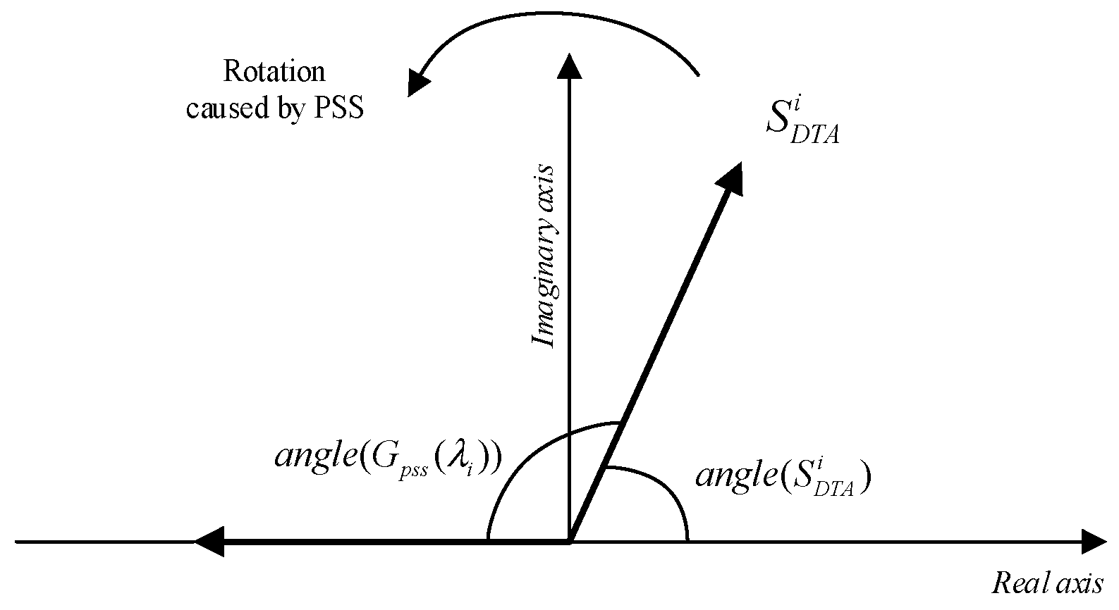
• On the basis of DTA theory, the damping torque index considering data corruption is obtained. The DTI can reflect the sensitivity of eigenvalues impacted by the WADC transfer function and thus, can be applied to execute wide-area signals selection and parameter tuning.

The rest of this paper is organized as follows. Section 2 illustrates the closed-loop linearized model with WAMS and proposes the unified model of data corruption. Combined with the second-order Pade approximation, the eigenvalue calculation model containing data-loss is derived. Section 3 deduces the DTI model containing data corruption and illustrates the method of WADC design. Section 4 validates the proposed model and method in the 2-area 4-machine (2A4M) system and Eastern China power grid (ECPG). Finally, Section 5 summarizes the conclusions of this paper.

2. Eigen-Analysis Model Considering Time-Delay and Data-Loss

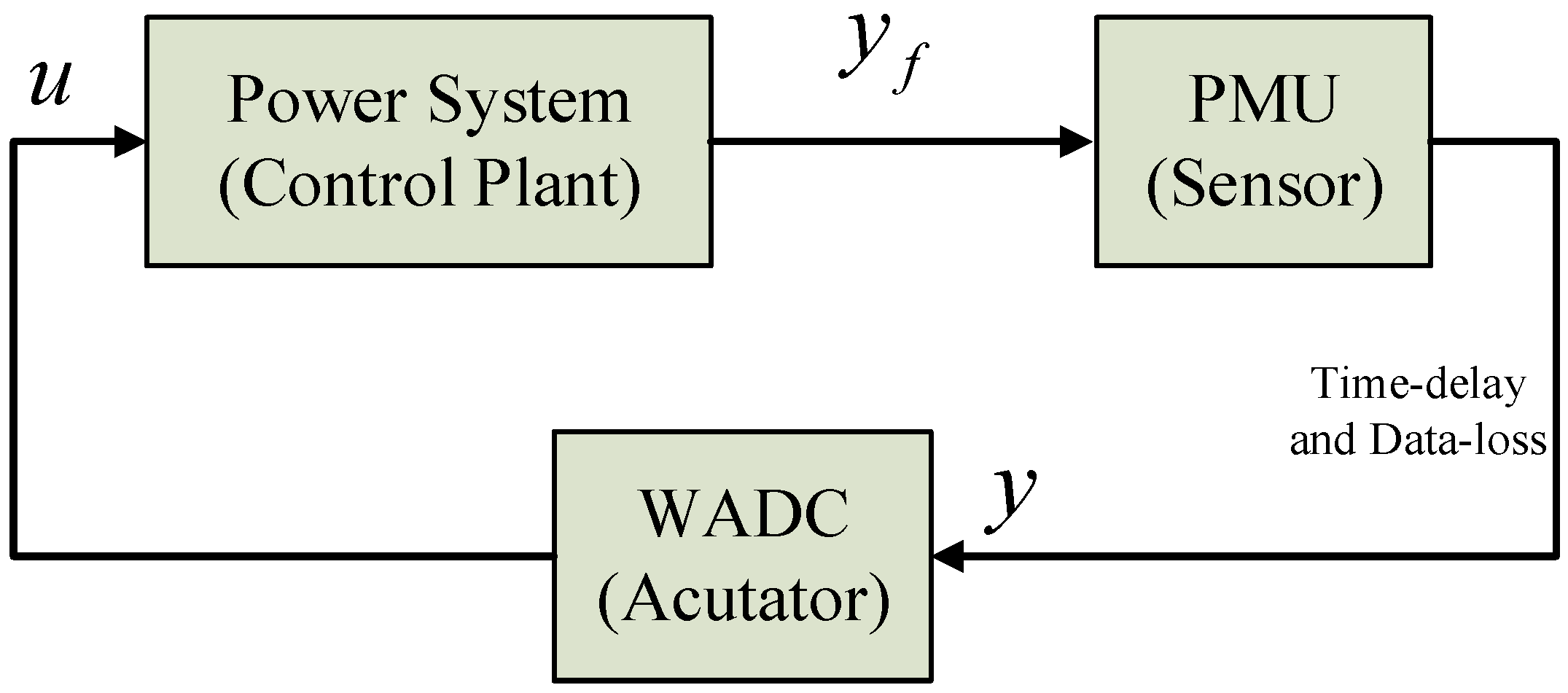
2.1. Closed-Loop Linearized Model with WAMS

The open-loop linearized model of power system is shown below [16]:

$$\{\begin{array}{c}\Delta \dot{X}=A\Delta X+B\Delta V\\ 0=C\Delta X+D\Delta V\end{array}$$

(1)

$$\Delta \dot{X}=A^{\prime }\Delta X$$

(2)

where $X\in {\Re }^n$ is the vector consisting of system state variables; $V$ is the voltage vector; and $A$, $B$, $C$, and $D$ are corresponding coefficient matrixes. By eliminating the terminal voltages in (1), (2) can be derived. $A^{\prime }$ is the deduced coefficient matrix, whose equation is given in (3):

$$A^{\prime }=A-B{D}^{-1}C.$$

(3)

An illustrative diagram of the power system with WAMS is depicted in Figure 1, where $y_f$ is the output signal of power system, and $u$ is the feedback signal. The PMU collects data from the power system and transfers it to the WADC. The input signal $y$ of WADC contains time-delay and data-loss characteristics.

The closed-looped model with WAMS is presented in (4), where $\Delta u$ is the linearized quantity of $u$. $E_x$ and $E_y$ are the corresponding coefficient matrices. $G(s)$ is the transfer function of the WADC. Because the feedback signal containing wide-area characteristics, the power system model with WAMS consists of transcendental equations [17] and is more complicated:

$$\{\begin{array}{c}\Delta \dot{X}=A\Delta X+B\Delta V+E_x\Delta u\\ 0=C\Delta X+D\Delta V+E_y\Delta u\\ \Delta u=G(s)\Delta y\end{array}.$$

(4)

2.2. Unified Mathematical Model of Time-Delay and Data-Loss

In contrast to the delay, data-loss is a probabilistic event. The data-loss ratio is the possibility that data-loss happens. The PMU collects data and transmits it to controllers discretely. Each sampling is an independent probability event. If data-loss does not happen, WADC can receive the newest data at this moment, i.e., $X_i(t-{\tau }_i)$. If the data is missing, WADC has to adopt the data received at the previous moment, i.e., $X_i(t-{\tau }_i-{\tau }_s)$. We assume that the input of WADC is comprised of $L$ signals, and the equations are summarized as follows:

$$y(t)=\{\begin{array}{l}{\displaystyle \sum _{i=1}^L{C}_i{X}_i(t-{\tau }_i-{\tau }_s),\text{data- loss happens}}\hfill \\ {\displaystyle \sum _{i=1}^L{C}_i{X}_i(t-{\tau }_i)},\text{data- loss donesn’t happens}\hfill \end{array}$$

(5)

where $C_i$ and ${\tau }_i$ are the respective signal coefficients and time-delay of the ith signal. ${\tau }_s$ is the time taken for the PMU sampling interval.

Obviously, the data collected by WADC are stochastic and thus, power system eigenvalues considering data-loss cannot be calculated directly. According to the mathematical expectation of data-loss, the equation can be transformed into

$$y(t)={\displaystyle \sum _{i=1}^L{C}_i({\gamma }_i{X}_i(t-{\tau }_i-{\tau }_s)+(1-{\gamma }_i)X_i(t-{\tau }_i))}$$

(6)

where ${\gamma }_i$ is the data-loss ratio of the ith signal. Equation (6) can be converted to the frequency domain to obtain

$$y(s)={\displaystyle \sum _{i=1}^L{C}_i({\gamma }_i{e}^{-({\tau }_i+{\tau }_s)s}+(1-{\gamma }_i)e^{-{\tau }_{i}s})}{X}_i(s).$$

(7)

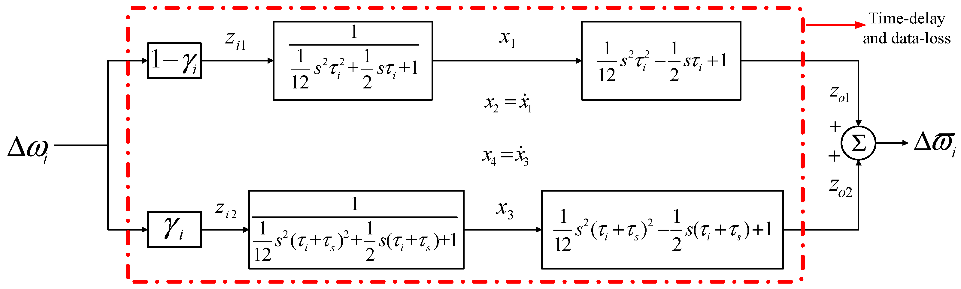
2.3. Pade Approximation

In the Laplace domain, time-delay can be represented by $e^{-\tau s}$, where $\tau$ is the time of delay. Pade approximation is an efficient rational polynomial method that is used to approach $e^{-\tau s}$ [18,19]. It is assumed that the numerator is an lth polynomial and the denominator is a kth one, and the approximation equation can be written as follows:

$$e^{-\tau s}\approx R(s)=\frac{N_l(s)}{N_k(s)}=\frac{a_0+a_1\tau s+\cdots a_l{(\tau s)}^l}{b_0+b_1\tau s+\cdots b_k{(\tau s)}^k}$$

(8)

where $a_j$ and $b_j$ are coefficients, and their equations are presented as follows:

$$a_j={(-1)}^j\frac{(l+k-j)!l!}{(l+k)!j!(l-j)!}$$

(9)

$$b_j=\frac{(l+k-j)!k!}{(l+k)!j!(k-j)!}.$$

(10)

In practical applications, normally $l=k$, the order of Pade approximation. Hwang [20] indicates that second-order Pade approximation can achieve sufficient accuracy and efficiency. Thus, this paper adopts the second-order model of Pade approximation which is shown in (11).

$$e^{-\tau s}\approx =\frac{1-\frac{1}{2}\tau s+\frac{1}{12}{(\tau s)}^2}{1+\frac{1}{2}\tau s+\frac{1}{12}{(\tau s)}^2}.$$

(11)

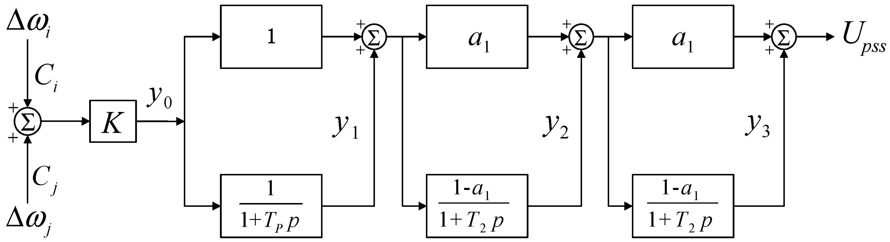
2.4. Linearized Model of Controller with Wide-Area Signals

Based on the proposed model of data corruption and second-order Pade approximation, the equation of sampling data can be transformed as shown below

$$\begin{array}{l}\Delta y(s)={\displaystyle \sum _{i=1}^L{C}_i\Delta }{\varpi }_i(s)={\displaystyle \sum _{i=1}^L{C}_i({\gamma }_i{e}^{-({\tau }_i+{\tau }_s)s}+(1-{\gamma }_i)e^{-{\tau }_{i}s})}\Delta {\omega }_i(s)\\ ={\displaystyle \sum _{i=1}^L{C}_i({\gamma }_i\frac{1-\frac{1}{2}({\tau }_i+{\tau }_s)s+\frac{1}{12}{(({\tau }_i+{\tau }_s)s)}^2}{1+\frac{1}{2}({\tau }_i+{\tau }_s)s+\frac{1}{12}{(({\tau }_i+{\tau }_s)s)}^2}+(1-{\gamma }_i)\frac{1-\frac{1}{2}{\tau }_{i}s+\frac{1}{12}{({\tau }_{i}s)}^2}{1+\frac{1}{2}{\tau }_{i}s+\frac{1}{12}{({\tau }_{i}s)}^2})}\Delta {\omega }_i(s)\end{array}$$

(12)

where $\Delta {\omega }_i$ is the feedback signal that the PMU transmits to the WADC, and $\Delta {\varpi }_i$ is the signal containing data corruption. In accordance with (12), the illustrative diagram of its linearized model is displayed in Figure 2, where $x_1$ to $x_4$ are additional state variables. $z_{i1}$, $z_{o1}$, $z_{i2}$, and $z_{o2}$ are additional algebraic variables.

Detailed equations are given as follows:

$$\{\begin{array}{l}{x}_2={\dot{x}}_1=\frac{d{x}_1}{dt}\\ z_{i1}=\Delta {\omega }_i(1-{\gamma }_i)\\ z_{i1}=\frac{1}{12}{\tau }_i^2{\dot{x}}_2+\frac{1}{2}{\tau }_j{x}_2+x_1\\ z_{o1}=\frac{1}{12}{\tau }_i^2{\dot{x}}_2-\frac{1}{2}{\tau }_j{x}_2+x_1\end{array}$$

(13)

$$\{\begin{array}{l}{x}_4={\dot{x}}_3=\frac{d{x}_3}{dt}\\ z_{i2}=\Delta {\omega }_i{\gamma }_i\\ z_{i2}=\frac{1}{12}{({\tau }_i+{\tau }_s)}^2{\dot{x}}_4+\frac{1}{2}({\tau }_i+{\tau }_s)x_4+x_3\\ z_{o2}=\frac{1}{12}{({\tau }_i+{\tau }_s)}^2{\dot{x}}_4-\frac{1}{2}({\tau }_i+{\tau }_s)x_4+x_3\end{array}.$$

(14)

After transformation and reduction, we can obtain

$$\{\begin{array}{l}{\dot{x}}_1=x_2\\ {\dot{x}}_2=\frac{12}{{\tau }_i^2}\Delta {\omega }_i(1-{\gamma }_i)-\frac{12}{{\tau }_i^2}{x}_1-\frac{6}{{\tau }_i}{x}_2\\ {\dot{x}}_3=x_4\\ {\dot{x}}_4=\frac{12}{{({\tau }_i+{\tau }_s)}^2}\Delta {\omega }_i{\gamma }_i-\frac{12}{{({\tau }_i+{\tau }_s)}^2}{x}_3-\frac{6}{({\tau }_i+{\tau }_s)}{x}_4\end{array}$$

(15)

$$\{\begin{array}{l}{z}_{o1}=\Delta {\omega }_i(1-{\gamma }_i)-{\tau }_i{x}_2\hfill \\ z_{o2}=\Delta {\omega }_i{\gamma }_i-({\tau }_i+{\tau }_s)x_4\hfill \end{array}.$$

(16)

The detailed sections of PSS are shown below, where $u_{pss}$ is the output of PSS to the excitation system, i.e., $u$ in Figure 1. $K$, $T_s$, $T_1$, and $T_2$ are corresponding parameters.

For demonstration purposes, this paper takes a WADC with two feedback signals as an example. $x_5$ to $x_8$, and $z_{i3}$, $z_{i4}$, and $z_{o3}$, $z_{o4}$ are the corresponding variables of signal $\Delta {\omega }_j$. In accordance with Figure 3, the linearized model of WADC is derived in Figure 4.

$y_1$, $y_2$, and $y_3$ are the auxiliary state variables of WADC and $a_1=T_1/T_2$. The differential equations of WADC are presented as follows:

$$\{\begin{array}{l}\begin{array}{l}\frac{d{y}_1}{dt}=\frac{1}{T_p}(-y_1+K{y}_0)\hfill \\ \frac{d{y}_2}{dt}=\frac{1}{T_2}\left[-y_2+(1-a_1)(K{y}_0-y_1)\right]\hfill \end{array}\hfill \\ \frac{d{y}_3}{dt}=\frac{1}{T_2}\left[-y_3+(1-a_1)y_2+a_1(1-a_1)(K{y}_0-y_1)\right]\hfill \\ y_0=C_i(\Delta w_i-{\tau }_i{x}_2-({\tau }_i+{\tau }_s)x_4)+C_j(\Delta w_j-{\tau }_j{x}_6-({\tau }_j+{\tau }_s)x_8)\hfill \\ \Delta U_{pss}=y_3+a_1{y}_2-a_1^2{y}_1+a_1^{2}K{y}_0\hfill \end{array}.$$

(17)

The above equations are added into the conventional power system state-space model, i.e., (4), to derive the eigenvalue calculation model of the power system containing time-delay and data-loss.

3. Wide-Area Damping Controller Design Based on the Damping Torque Index

3.1. Damping Torque Index Considering Time-Delay and Data-Loss

In DTA theory, DTI is defined to indicate the sensitivity of one eigenvalue, ${\lambda }_i$, to $G_{pss}(s)$. As depicted in Figure 3, the equation is as follows:

$$G_{pss}(s)=K\frac{T_{s}s}{1+T_{s}s}{(\frac{1+T_{1}s}{1+T_{2}s})}^2.$$

(18)

DTI can clearly demonstrate how PSS and its parameters affect the oscillation mode. The equations are presented below [21,22,23]:

$$S_{DTA}^i=\frac{\Delta {\lambda }_i}{\Delta G_{pss}({\lambda }_i)}={\displaystyle \sum _{j=1}^N{S}_{ij}{M}_j{H}_{ij}\angle {\phi }_{ij}}$$

(19)

where $S_{ij}$ is the sensitivity of the oscillation mode to the damping torque coefficient on the jth generator, $T_{Dij}$, as presented in (20). $M_j$ is the inertia parameter of the jth generator. $H_{ij}\angle {\phi }_{ij}$ is the damping torque that PSS contributes to the jth generator, and the equation is given in (21).

$$S_{ij}=\frac{\partial {\lambda }_i}{\partial T_{Dij}}$$

(20)

$$H_{ij}\angle {\phi }_{ij}=B_s({\lambda }_i){\gamma }_j({\lambda }_i)=B_s({\lambda }_i)\frac{C_{ki}{V}_i}{V_{i2j}}$$

(21)

where $B_s({\lambda }_i)$ is the transfer function from PSS to the jth generator electromechanical oscillation loop. ${\gamma }_j({\lambda }_i)$ is the coefficient matrix of the PSS output after signal reconstruction. Its single signal equation is presented in (22):

$${\gamma }_j({\lambda }_i)=\frac{\Delta y}{\Delta {\omega }_j}=\frac{X({\lambda }_i)}{\Delta {\omega }_j}=\frac{C_{ki}{V}_i}{V_{i2j}}$$

(22)

where $C_{ki}$ is the coefficient of the reconstruction signal. $V_i$ is the right eigenvector of ${\lambda }_i$. The detailed mechanism and derivation process are available in [22,23,24]. Therefore, the conventional equation of DTI of single signal is derived by

$$S_{DTA}^i={\displaystyle \sum _{j=1}^N{S}_{ij}{M}_j{B}_s({\lambda }_i)\frac{C_{ki}{V}_i}{V_{i2j}}}.$$

(23)

Obviously, the characteristics of data corruption are embodied at the signal reconstruction matrix, ${\gamma }_j({\lambda }_i)$. For the WADC input consisting of multiple signals, according to (7), we have

$${\gamma }_j({\lambda }_i)=\frac{\Delta y}{\Delta {\omega }_j}=\frac{{\displaystyle \sum _{p=1}^L{C}_p({\gamma }_p{e}^{-({\tau }_p+{\tau }_s){\lambda }_i}+(1-{\gamma }_p)e^{-{\tau }_p{\lambda }_i})}{X}_p({\lambda }_i)}{\Delta {\omega }_j}={\displaystyle \sum _{p=1}^L\frac{C_p({\gamma }_p{e}^{-({\tau }_p+{\tau }_s){\lambda }_i}+(1-{\gamma }_p)e^{-{\tau }_p{\lambda }_i})C_{ki}{V}_i}{V_{i2j}}}.$$

(24)

Thus, the DTI containing time-delay and data-loss is derived:

$$S_{DTA}^i={\displaystyle \sum _{j=1}^N{S}_{ij}{M}_j{B}_s({\lambda }_i){\displaystyle \sum _{p=1}^L\frac{C_p({\gamma }_p{e}^{-({\tau }_p+{\tau }_s){\lambda }_i}+(1-{\gamma }_p)e^{-{\tau }_p{\lambda }_i})C_{ki}{V}_i}{V_{i2j}}}}.$$

(25)

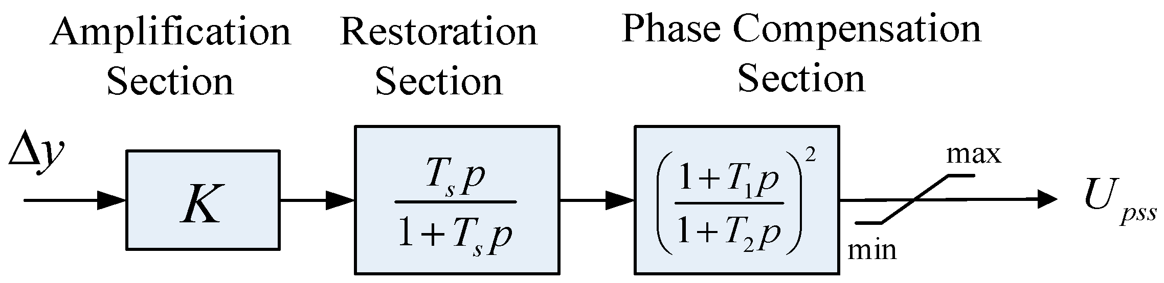
3.2. Wide-Area Damping Controller Design

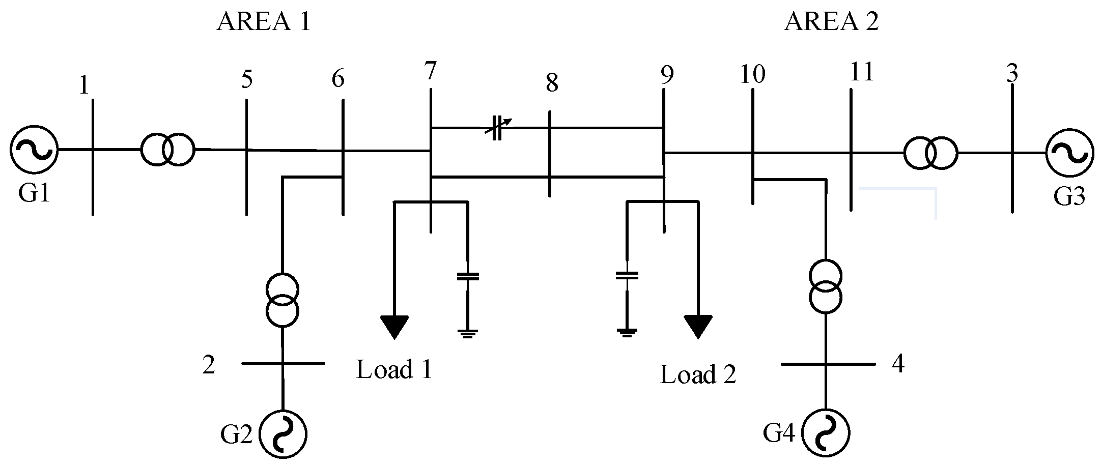
WADC design includes the selection of feedback signals and controller parameter tuning. According to DTA theory, DTI is defined to evaluate the impact of the controller transfer function on one objective mode and thus can reflect the influence of WADC with different feedback signals on eigenvalues. This means that the WADC adopting the feedback signal with the biggest DTI can exert the biggest impact on the objective mode.

For a WADC installed at the jth generator, the variation of the ith mode is calculated as below:

$$\Delta {\lambda }_i=S_{DTA}^i\Delta G_{pss}({\lambda }_i).$$

(26)

As shown in Figure 5, the most efficient method to damp the mode is to move the ith mode horizontally to the left side with its frequency constant [25]. Therefore, the phase compensation of controller can be derived by

$$angle(G_{pss}({\lambda }_i))={180}^{\circ }-angle(S_{DTA}^i).$$

(27)

The phase adjustment of PSS mainly depends on the phase compensation section, including $T_1$ and $T_2$. In conventional applications of signal selection and WADC parameter tuning, the open-loop eigenvalues are used to approximate the close-loop values and are not very precise. By using the proposed eigenvalue and DTI calculation model containing time-delay and data-loss, the process is more accurate and effective for WADC design.

4. Case Study

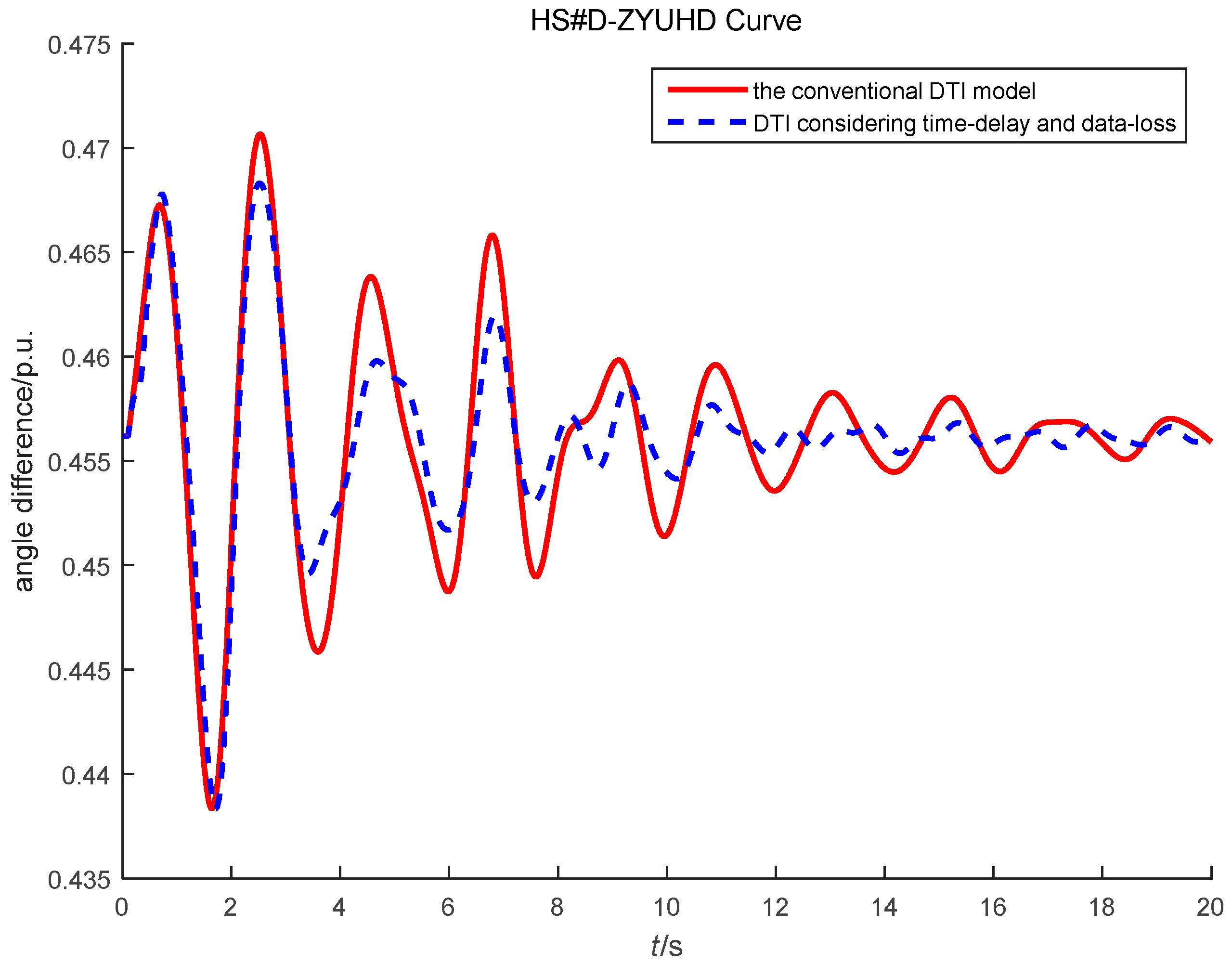
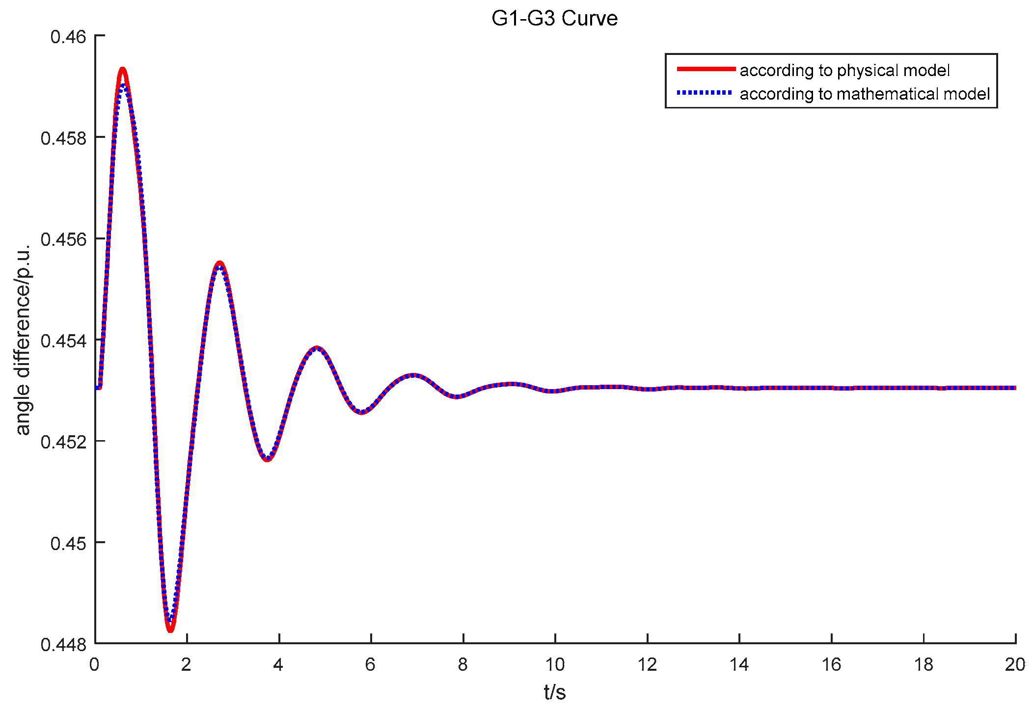
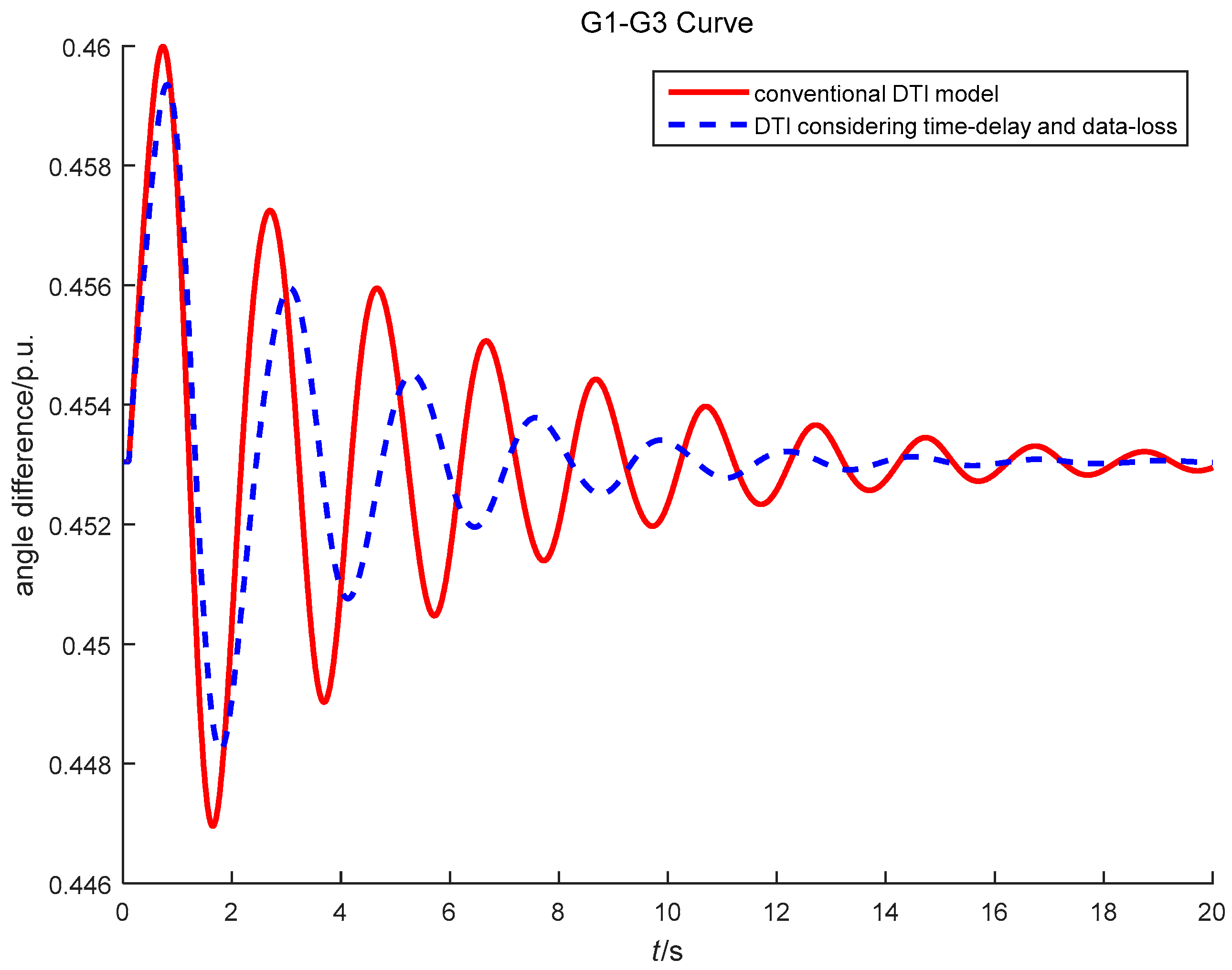
4.1. Simulations of Different Models of Data-Loss

Firstly, the 2A4M Kundur system (Figure 6) was simulated to verify the proposed model. The detailed parameters are available in [26]. There are three electromechanical oscillation modes in this system. Among them, the inter-area mode, ${\lambda }_1$, exerts a great impact on the system’s stability.

The WADC was installed at G1 and the feedback signal was $\Delta {\delta }_1-\Delta {\delta }_3$, where $\delta$ is the generator power angle and $K=10$, $T_s=5$, $T_1=0.5$, and $T_2=0.05$. In order to validate the unified model of data corruption, data-loss was simulated respectively using the physical model and mathematical model. For the physical model, one random number was generated between 0 and 1. If it was more than the data-loss ratio, the controller received the updated data. Otherwise, the data of the previous moment was adopted. As for the mathematical model, the input of WADC was directly calculated according to (6). A three-phase, short-circuit fault occurred at B8 and was cleared 0.01 s later. Figure 7 presents the comparative simulation curves of the G1–G3 angle difference according to the different models of data-loss.

Figure 7 shows there was no prominent difference between the two curves associated with two different models, which demonstrates the correctness of the unified mathematic model in (6).

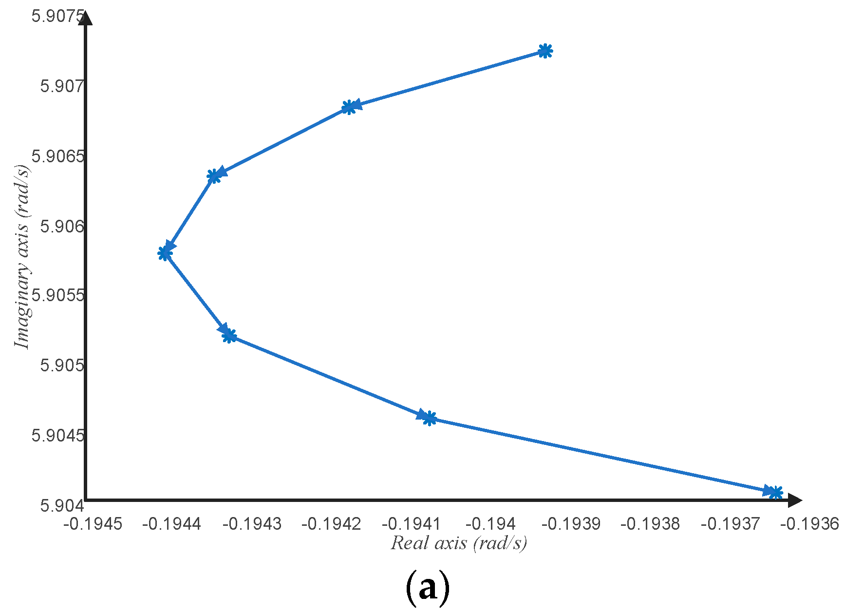
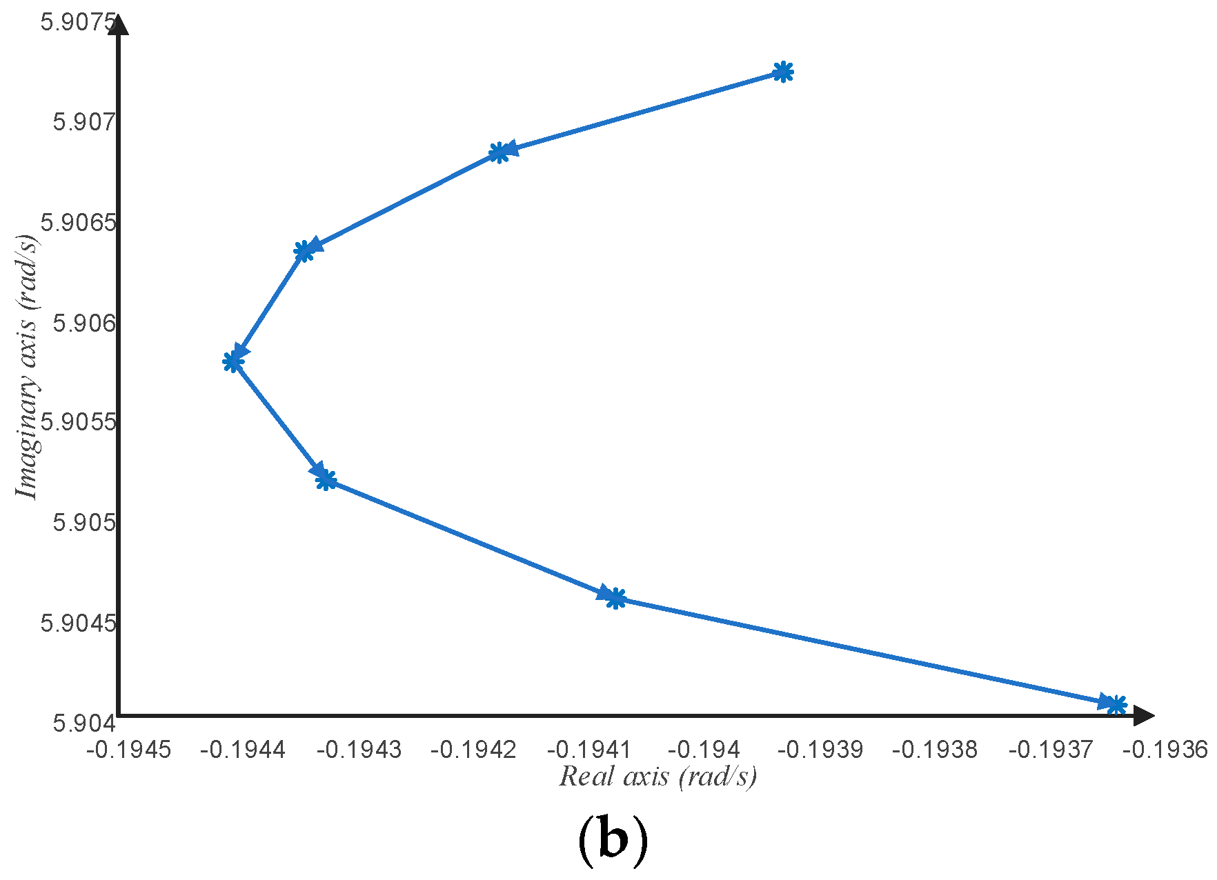
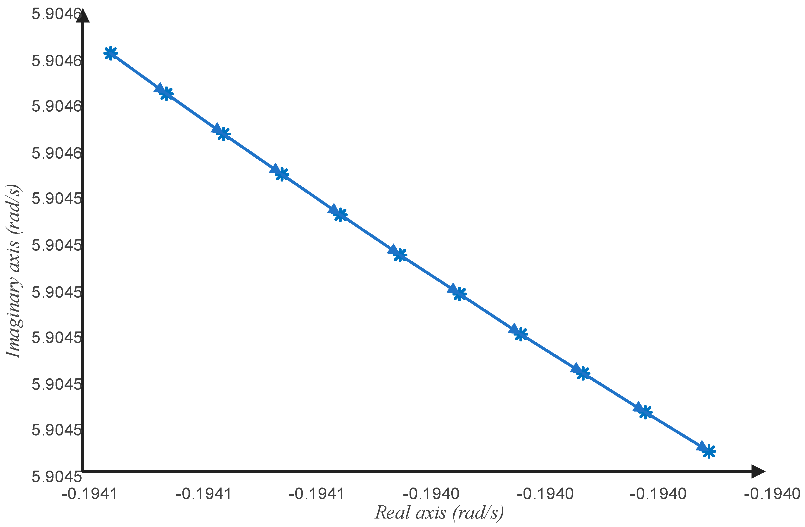
4.2. Impact Mechanism

Firstly, to investigate the impact of time-delay, ${\tau }_1={\tau }_3$ was kept and their values were assigned to be 0 s to 0.4 s and ${\gamma }_1={\gamma }_3=0.1$. Time-domain simulations and eigenvalue calculation were carried out with different time-delays. The simulation curves and the modal trajectory of ${\lambda }_1$ are displayed in Figure 8 and Figure 9.

According to Figure 9, when time-delay was from 0 s to 0.24 s, the variation of ${\lambda }_1$ was very small. With an increase in the delay, the real part moved first to the left and then to the right. This means that the increase in time-delay did not exert a negative impact on the stability at first. Once time-delay was over 0.28 s, the real part rapidly grew to greater than 0 which meant that the system was no longer stable. Obviously, a time-delay margin existed near 0.28 s. The simulation curves in Figure 8 are consistent with the modal trajectory.

The time-delay constant was maintained at ${\tau }_1={\tau }_3=0.2\mathrm{s}$. The simulations and modal trajectory analysis were conducted with different data-loss ratios, from 0 to 0.2, and the results are shown in Figure 10 and Figure 11.

It is revealed in the figures that data-loss also has a negative influence on system stability and the curve presents a monotonous characteristic. However, the modal variation was not very significant compared with the time-delay. This is consistent with the unified model of data corruption for data-loss, which generates a time-delay of ${\gamma }_i{\tau }_s$, which is smaller than ${\tau }_i$. The simulation curves in Figure 10 show this characteristic as well.

4.3. Controller Signal Selection and Parameter Tuning

The WADC was installed at G1 to damp the inter-area mode, ${\lambda }_1$. Four feedback signals were considered including differences in G1–G3 angular velocities, power angles, and active powers and B7–B9 active powers. Their characteristics and the DTI calculation results are presented in

Table 1. Characteristics and DTI results of different feedback signals.

Feedback Signal	Time-Delay/s	Data-Loss Ratio	Time-Delay/s	Data-Loss Ratio	Abs (DTI)/p.u.	Angle (DTI)/°
$\Delta {\omega }_1-\Delta {\omega }_3$	0.08 ($\Delta {\omega }_1$)	0.1 ($\Delta {\omega }_1$)	0.08 ($\Delta {\omega }_3$)	0.1 ($\Delta {\omega }_3$)	0.0006	−62.35
$\Delta {\delta }_1-\Delta {\delta }_3$	0.08 ($\Delta {\delta }_1$)	0.1 ($\Delta {\delta }_1$)	0.08 ($\Delta {\delta }_3$)	0.1 ($\Delta {\delta }_3$)	0.0042	−157.54
$\Delta P_{G1}-\Delta P_{G3}$	0.08 ($\Delta P_{G1}$)	0.1 ($\Delta P_{G1}$)	0.08 ($\Delta P_{G3}$)	0.1 ($\Delta P_{G3}$)	0.1856	−145.32
$\Delta P_{B7}-\Delta P_{B9}$	0.06 ($\Delta P_{B7}$)	0.1 ($\Delta P_{B7}$)	0.06 ($\Delta P_{B9}$)	0.1 ($\Delta P_{B9}$)	0.1058	−150.97

.

Table 1 shows that every signal has the effect of damping the objective mode. Among them, the signal, $\Delta P_{G1}-\Delta P_{G3}$, showed the best effect followed by $\Delta P_{B7}-\Delta P_{B9}$. Thus, $\Delta P_{G1}-\Delta P_{G3}$ was selected to be the input signal of WADC.

$T_1$, the parameter of the phase compensation element, exerts great impacts on the system’s dynamic stability and needs to be tuned. The other parameters—PSS, $K$, $T_s$, and $T_2$—are usually set according to experience.

$K=10$, $T_s=5$, $T_2=0.05$, and the closed-loop eigenvalues were calculated. According to the DTI and the eigenvalue, $T_1$ was calculated to be 0.45381 by using the phase compensation method. Then, the method was conducted according to the conventional DTI. The obtained value was $T_1=0.16938$. The two parameters were applied to the WADC, an eigen-analysis and simulations were conducted. The results are presented in

Table 2. Objective mode tuned by different models.

Model	Real Part/Rad/s	Imaginary Part/Rad/s	Frequency/Hz	Damping Ratio
The conventional model	−0.19421	5.9067	0.9401	0.03278
The proposed model	−0.34402	2.8285	0.4502	0.1193

and Figure 12. As shown in Figure 12, the proposed tuning method more efficiently inhibited the inter-area mode and improved the system’s small-signal stability.

In this study, WADC was tuned to damp the objective oscillation mode in power systems containing data-loss. It has a clearer physical meaning and damping objective compared to the controller in [14], which was designed to compensate the negative influence of data-loss in the process of data sampling and transmission.

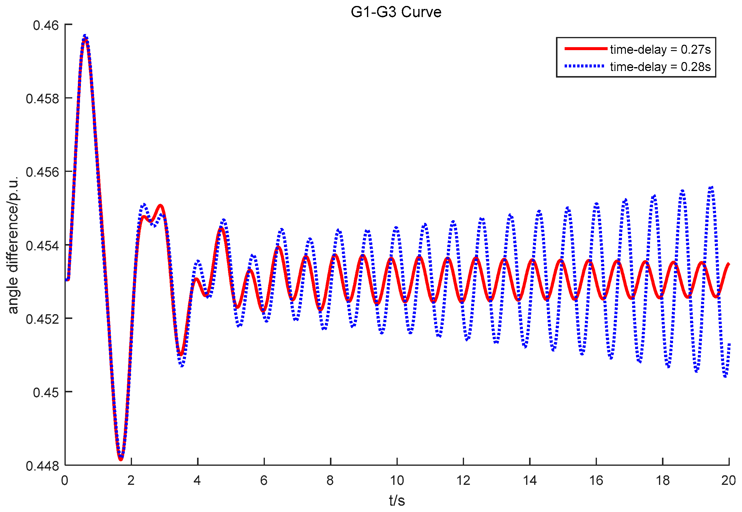
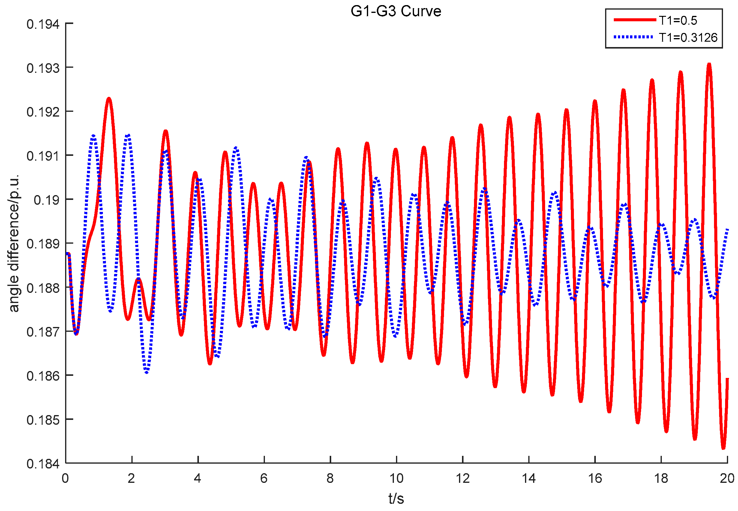
4.4. System Stability Time-Delay Margin Calculation

When the WADC was at G1, the feedback signal was $\Delta {\delta }_1-\Delta {\delta }_3$ and $K=10$, $T_s=5$, $T_1=0.5$, and $T_2=0.05$. The time-delay was increased and the eigenvalue of ${\lambda }_1$ was calculated. When the real part is 0, the delay obtained is the stability margin, which means the system is asymptotically stable. In this case, the margin value obtained was 0.2736 s. Simulations were carried out with time-delays of 0.27 s and 0.28 s (Figure 13). Obviously, the system lost its dynamic stability when the time-delay reached 0.28 s.

Then, WADC parameter tuning was conducted and $T_1=0.3126$ was derived. Simulations were conducted with this parameter, and Figure 14 displays the comparative curves. It was revealed that the tuned parameter made the system resume its stability which demonstrates that the proposed method can extend the system’s delay margin and thus enhance its dynamic stability.

Then, the WADC was installed at G3 with the signal $\Delta {\delta }_3-\Delta {\delta }_1$ and the same parameters as the controller in G1. The margin was calculated to be 0.2537 s, which means that the WADC located at G1 had a better damping effect compared to that at G3. Thus, the margin can be an index for selecting the WADC location and feedback signals.

4.5. WADC Parameter Tuning in ECPG

Then, the method was applied in a real, large-scale system, the ECPG. This system consists of 64 generators, 294 nodes, and 628 lines. There are 63 modes in this system, among them, Mode FJ, which has a frequency 0.477 Hz, is an important mode and is poorly damped. The detailed parameters of ECPG are available in [27].

In accordance with the results of participation factors and controllability, WADC was installed at HS#D (G54). The feedback signal was selected to be the difference in power angle between GYC_D1 and GYC_D2, namely $\Delta {\omega }_{23}-\Delta {\omega }_{24}$. ${\tau }_{23}=0.1\mathrm{s}$, ${\gamma }_{23}=0.2$, ${\tau }_{24}=0.12\mathrm{s}$, and ${\gamma }_{24}=0.1$

WADC was tuned by the conventional and proposed methods. The results were 0.3157 and 0.5124 respectively. The eigen-analysis and simulations were carried out and are displayed in

Table 3. Objective mode tuned by different models in the Eastern China power grid (ECPG).

Mode	Real Part/Rad/s	Imaginary Part/Rad/s	Frequency/Hz	Damping Ratio
The conventional model	−0.18688	4.4643	0.7105	0.04183
The proposed model	−0.25484	4.8136	0.7661	0.05287

and Figure 15. The results demonstrate the proposed method effectively dampened the inter-area oscillation in ECPG as well.

Then, the time-delay margin calculation was conducted in this system. The WADC was at G54 with the signal $\Delta {\omega }_{23}-\Delta {\omega }_{24}$ and ${\gamma }_{23}={\gamma }_{24}=0$. The margin was 0.3067 s, which means it had a better tolerance to time-delay in ECPG than the 2A4M system. Thus, the ECPG is was shown to be more stable than the 2A4M system with the above WADC locations and parameters. Therefore, to some extent, the margin can be considered as a parameter to assess the stability of different systems.

5. Conclusions

The current investigation mainly focused on the impact brought about by data-loss and controller design to eliminate the negative impact based on some control methods of the nonlinear system, for example, the Lyapunov-based controller which has a better robustness and effect. These investigations showed that the proposed method in our paper can calculate the eigenvalues and DTI considering data-loss, which has a clear physical meaning and allows the analysis of the detailed impact mechanism. It can also the calculate system delay margin and be applied to design the WADC to suppress inter-area oscillations. Some conclusions from the model analysis and case study are as follows:

(1)

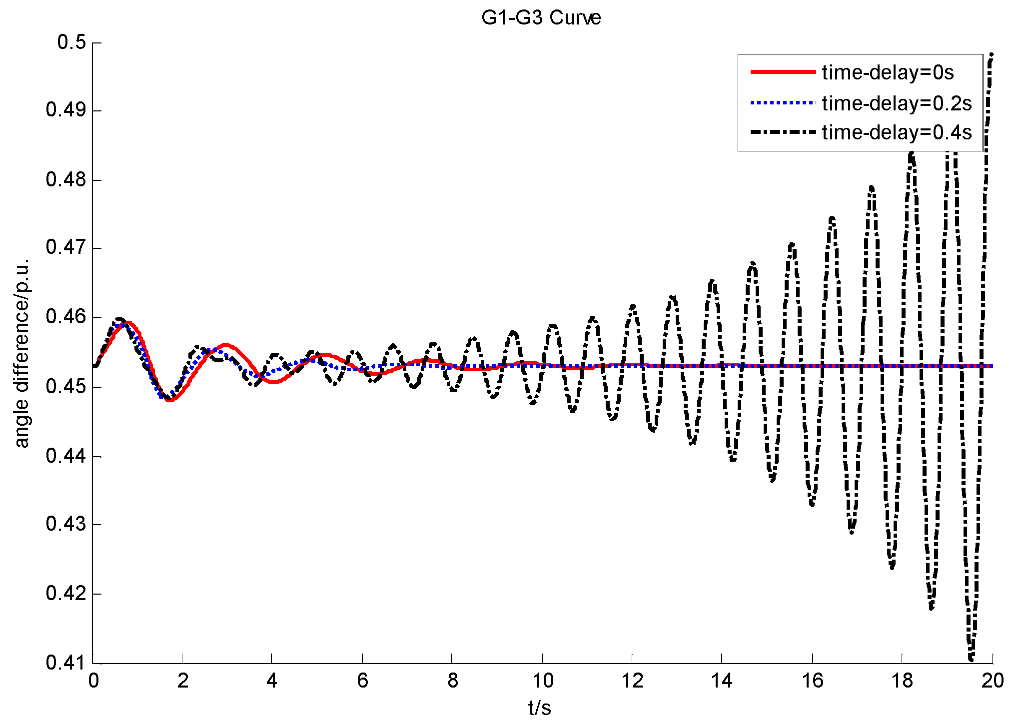
The impact mechanism of the time-delay on small-signal dynamics is complicated. An increase in the time-delay may increase the damping of one oscillation mode when it is relatively small. However, when the time-delay is over the stability margin, system stability will get worse rapidly.

(2)

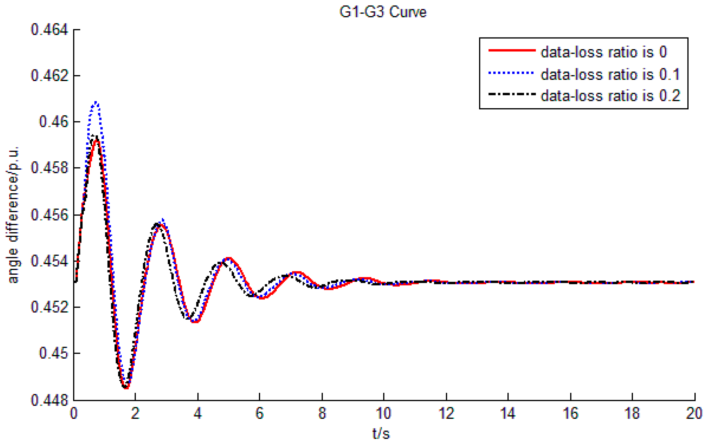
Data-loss can reduce the delay margin and system stability. However, the impact is relatively small as it generates an equivalent time-delay of ${\gamma }_i{\tau }_s$. Therefore, in practical applications, more attention should be paid to the negative impact brought about by time-delay than data-loss.

(3)

The system delay margin can be derived by using the proposed eigenvalue calculation model. It is an important parameter of the power system and is helpful for wide-area device improvement and signal selection. The parameter tuning method of WADC based on DTI can extend the system’s time-delay margin and thus enhance system dynamic performance.

In this paper, the WADC was designed to deal with fixed time-delay and data-loss. In practical applications, both time-delay and data-loss may be time-varying and stochastic. In addition, different types of delay, such as single data-loss or continuous data-loss, may exist and these deserve further research. Therefore, the time-varying and stochastic characteristics of data corruption and different delay types will be one of our future research directions.

References

1. Wu, X.; Dorfler, F.; Jovanovic, M.R. Input-Output Analysis and Decentralized Optimal Control of Inter-Area Oscillations in Power Systems. IEEE Trans. Power Syst. 2016, 31, 2434–2444. [Google Scholar] [CrossRef]
2. Nezam Sarmadi, S.A.; Venkatasubramanian, V.; Salazar, A. Analysis of November 29, 2005 Western American Oscillation Event. IEEE Trans. Power Syst. 2016, 31, 5210–5211. [Google Scholar] [CrossRef]
3. Che, Y.; Xu, J.; Shi, K.; Liu, H.; Chen, W.; Yu, D. Stability analysis of aircraft power systems based on a unified large signal model. Energies 2017, 10, 1–15. [Google Scholar] [CrossRef]
4. Salimian, M.R.; Aghamohammadi, M.R. Intelligent out of Step Predictor for Inter Area Oscillations Using Speed-Acceleration Criterion as a Time Matching for Controlled Islanding. IEEE Trans. Smart Grid 2018, 9, 2488–2497. [Google Scholar] [CrossRef]
5. Khandeparkar, K.V.; Soman, S.A.; Gajjar, G. Detection and Correction of Systematic Errors in Instrument Transformers Along with Line Parameter Estimation Using PMU Data. IEEE Trans. Power Syst. 2017, 32, 3089–3098. [Google Scholar] [CrossRef]
6. Liao, K.; Wang, Y. A comparison between voltage and reactive power feedback schemes of DFIGs for inter-Area oscillation damping control. Energies 2017, 10, 1206. [Google Scholar] [CrossRef]
7. Preece, R.; Milanović, J.V.; Almutairi, A.M.; Marjanovic, O. Damping of inter-area oscillations in mixed AC/DC networks using WAMS based supplementary controller. IEEE Trans. Power Syst. 2013, 28, 1160–1169. [Google Scholar] [CrossRef]
8. Yao, W.; Jiang, L.; Wen, J.; Wu, Q.H.; Cheng, S. Wide-area damping controller of Facts devices for inter-area oscillations considering communication time delays. IEEE Trans. Power Syst. 2014, 29, 318–329. [Google Scholar] [CrossRef]
9. Zhu, K.; Chenine, M.; Nordström, L. ICT Architecture Impact on Wide Area Monitoring and Control Systems’ Reliability. IEEE Trans. Power Deliv. 2011, 26, 2801–2808. [Google Scholar] [CrossRef]
10. Huang, D.; Chen, Q.; Ma, S.; Zhang, Y.; Chen, S. Wide-Area Measurement—Based Model-Free Approach for Online Power System Transient Stability Assessment. Energies 2018, 11, 958. [Google Scholar] [CrossRef]
11. Yang, B.; Sun, Y. A novel approach to calculate damping factor based delay margin for wide area damping control. IEEE Trans. Power Syst. 2014, 29, 3116–3117. [Google Scholar] [CrossRef]
12. Cai, G.; Yang, D.; Liu, C. Adaptive wide-area damping control scheme for smart grids with consideration of signal time delay. Energies 2013, 6, 4841–4858. [Google Scholar] [CrossRef]
13. Li, J.; Chen, Z.; Cai, D.; Zhen, W.; Huang, Q. Delay-Dependent Stability Control for Power System with Multiple Time-Delays. IEEE Trans. Power Syst. 2016, 31, 2316–2326. [Google Scholar] [CrossRef]
14. Jungers, R.M.; Kundu, A.; Heemels, W.P.M.H. Observability and Controllability Analysis of Linear Systems Subject to Data Losses. IEEE Trans. Automat. Contr. 2017, 63, 3361–3376. [Google Scholar] [CrossRef]
15. Li, C.; Li, G.; Wang, C.; Du, Z. Eigenvalue Sensitivity and Eigenvalue Tracing of Power Systems with Inclusion of Time Delays. IEEE Trans. Power Syst. 2018, 33, 3711–3719. [Google Scholar] [CrossRef]
16. Wang, X.; Song, Y.; Irying, M. Modern Power Systems Analysis; Springer: Berlin, Germany, 2011. [Google Scholar]
17. Li, Y.; Geng, G.; Jiang, Q. An Efficient Parallel Krylov-Schur Method for Eigen-Analysis of Large-Scale Power Systems. IEEE Trans. Power Syst. 2016, 31, 920–930. [Google Scholar] [CrossRef]
18. Sinha, N.K.; Bereznai, G.T. Optimum approximation of high-order systems by low-order models. Int. J. Control 1971, 14, 951–959. [Google Scholar] [CrossRef]
19. Nie, Y.; Zhang, P.; Ma, Y.; Zhang, Y.; Fang, B.; Lv, D. Time delay trajectory analysis of modes in wide-area power system based on Pade approximation. Dianli Xitong Zidonghua Autom. Electr. Power Syst. 2018, 42, 87–92. (In Chinese) [Google Scholar] [CrossRef]
20. Hwang, C.; Lee, Y.C. Multifrequency Pade approximation via Jordan continued-fraction expansion. IEEE Trans. Autom. Contr. 1989, 34, 444–446. [Google Scholar] [CrossRef]
21. Gurrala, G.; Sen, I. Synchronizing and damping torques analysis of nonlinear voltage regulators. IEEE Trans. Power Syst. 2011, 26, 1175–1185. [Google Scholar] [CrossRef]
22. Zhou, T.; Chen, Z.; Guo, R.X. Power System Stabilizer Parameter Tuning Based on Closed-loop Damping Torque Analysis Method. Autom. Electr. Power Syst. 2016, 40, 56–60. (In Chinese) [Google Scholar] [CrossRef]
23. Li, H.F.; Du, W.; Wang, H.F.; Xiao, L.Y. Damping torque analysis of energy storage system control in a multi-machine power system. IEEE PES Innov. Smart Grid Technol. Conf. Eur. 2011, 1–8. [Google Scholar] [CrossRef]
24. Du, W.; Bi, J.; Lv, C.; Littler, T. Damping torque analysis of power systems with DFIGs for wind power generation. IET Renew. Power Gener. 2017, 11, 10–19. [Google Scholar] [CrossRef] [Green Version]
25. Zhang, J.; Chung, C.Y.; Han, Y. A novel modal decomposition control and its application to PSS design for damping interarea oscillations in power systems. IEEE Trans. Power Syst. 2012, 27, 2015–2025. [Google Scholar] [CrossRef]
26. Klein, M.; Rogers, G.J.; Kundur, P. A fundamental study of inter-area oscillations in power systems. IEEE Trans. Power Syst. 1991, 6, 914–921. [Google Scholar] [CrossRef]
27. Wang, C.; Li, J.; Li, L.; Sun, W.; Ni, Q.; Zhang, J. Low frequency oscillation characteristics of east china power grid after commissioning of huainan-shanghai uhv project. Dianli Xitong Zidonghua Autom. Electr. Power Syst. 2013, 37, 120–125. (In Chinese) [Google Scholar] [CrossRef]
Figure 1. Illustrative diagram of the power system with a wide-area measurement system (WAMS). WADC: wide-area damping controller.
Energies 11 03186 g001
Figure 2. Linearized model of the feedback signal.
Energies 11 03186 g002
Figure 3. Diagram of the power system stabilizer (PSS) transfer function.
Energies 11 03186 g003
Figure 4. Linearized model of the WADC.
Energies 11 03186 g004
Figure 5. Effect of phase compensation of the PSS.
Energies 11 03186 g005
Figure 6. Network of the 2-area 4-machine (2A4M) system.
Energies 11 03186 g006
Figure 7. Comparative simulation curves of the G1–G3 angle difference according to the different models of data-loss.
Energies 11 03186 g007
Figure 8. G1–G3 angle difference curves with different time-delays.
Energies 11 03186 g008
Figure 9. Modal trajectory regulated by time-delay: (a) 0 s to 0.24 s, (b) 0.28 s to 0.4 s.
Energies 11 03186 g009aEnergies 11 03186 g009b
Figure 10. G1–G3 angle difference curves with different data-loss ratios.
Energies 11 03186 g010
Figure 11. Modal trajectory regulated by the data-loss ratio (0 to 0.2).
Energies 11 03186 g011
Figure 12. Plots of power angle differences between G1 and G3 tuned by different models.
Energies 11 03186 g012
Figure 13. G1–G3 power angle difference curves with time-delays near the threshold.
Energies 11 03186 g013
Figure 14. G1–G3 power angle difference curves before and after tuning.
Energies 11 03186 g014
Figure 15. Plots of power angle differences in ECPG.
Energies 11 03186 g015