Driving Cycles Based on Fuel Consumption

Abstract

Type-approval driving cycles currently available, such as the Federal Test Procedure (FTP) and the Worldwide harmonized Light vehicles Test Cycle (WLTC), cannot be used to estimate real fuel consumption nor emissions from vehicles in a region of interest because they do not describe its local driving pattern. We defined a driving cycle (DC) as the time series of speeds that when reproduced by a vehicle, the resulting fuel consumption and emissions are similar to the average fuel consumption and emissions of all vehicles of the same technology driven in that region. We also declared that the driving pattern can be described by a set of characteristic parameters (CPs) such as mean speed, positive kinetic energy and percentage of idling time. Then, we proposed a method to construct those local DC that use fuel consumption as criterion. We hypothesized that by using this criterion, the resulting DC describes, implicitly, the driving pattern in that region. Aiming to demonstrate this hypothesis, we monitored the location, speed, altitude, and fuel consumption of a fleet of 15 vehicles of similar technology, during 8 months of normal operation, in four regions with diverse topography, traveling on roads with diverse level of service. In every region, we considered 1000 instances of samples made of m trips, where m varied from 4 to 40. We found that the CPs of the local driving cycle constructed using the fuel-based method exhibit small relative differences (<15%) with respect to the CPs that describe the driving patterns in that region. This result demonstrates the hypothesis that using the fuel based method the resulting local DC exhibits CPs similar to the CPs that describe the driving pattern of the region under study.

1. Introduction

Currently, there is a need for local driving cycles. Existing type-approval driving cycles do not describe correctly the driving patterns of a region of interests causing large differences between the fuel consumption (FC) observed during every day normal use of the vehicle in that region and the FC reported by the manufactures [1].

At present, there is not a clear definition for driving patterns. This term is used vaguely to describe the way drivers drive. Authors describe driving patterns in terms of a set of characteristic parameters (CPs), also known as performance values (PVs). They are speed-time based variables such as average speed, percentage of idling time, average positive acceleration, positive kinetic energy, etc. It remains unclear which set of CPs properly describes a driving pattern but there is an agreement among authors that driving patterns influence vehicle fuel consumption [2,3].

Driving cycles (DC) are time series of speeds that represent driving patterns [2,4] They have been constructed in the way that the values of the CPs of the DC are approximately equal to the values of the CPs that describe the driving patterns. DCs describe the workloads imposed on the vehicles and therefore have been used for assessing the environmental impact of traffic [5], and for optimizing new vehicles’ powertrain configurations and engine control strategies to reduce fuel consumption (FC) [6]. In this manuscript, we distinguish two types of DC: local and type-approval DC.

Presently, the Worldwide harmonized Light vehicles Test Cycle (WLTC) and the Federal Test Procedure (FTP), are some of the most well-known type-approval DCs [7,8,9]. These two DCs, as all type-approval DCs, are mainly used for the determination of vehicles’ fuel consumption and the mass emission of air pollutants, for comparative and certification processes [10,11,12] Manufactures report the measured fuel consumption when the vehicle follows a type-approval DC as part of the introduction process of a new technology in the vehicles market [13,14]. However, these existing type-approval DCs do not describe correctly the real-world driving patterns of any particular region.

The key issue relative to local DCs is their representativeness of the real-world local driving patterns. Researchers look for DCs that provide a synthesized representation of the local driving patterns [5,15,16].

Two main approaches have been used to construct DCs. The first one is the micro-trips-based approach in which a large sample of time series of speeds (trips) are divided into micro-segments (known as micro-trips) which are speed vs. time sections with initial and final speeds equal to zero. Then, a set of micro-trips are selected “quasi-randomly” and spliced together to form a candidate representative DC. A clustering step is occasionally applied for gathering micro-trips with similar speed-acceleration values. The selected DC is the one with CPs values similar to the respective average values of CPs of the trips collected. LA92, Singapore, Hong Kong and Bangkok DCs were obtained with this micro-trips approach [12,15,17].

The second approach to construct DCs is based on Markov theory and uses the Monte Carlo technique. Some examples are found in [15,18,19]. In this second approach, speed and acceleration ranges are discretized into n and m sections, respectively. They configure a matrix of n x m states. The measured values of speed and acceleration from all the sampled trips are grouped into those states, forming the speed acceleration frequency distribution (SAFD) or the speed acceleration probability distribution (SAPD) when the SAFD is normalized. Next, an [(nxm) x (nxm)] probability transition matrix is computed. Similar to the SAPD, those probabilities are computed by counting the number the times that vehicles moved from one state to another and then normalizing with respect to the total number of transitions. Then, the Monte Carlo simulation technique is used to produce a candidate DC. The process consists of using a random number to select the next state in a manner in which transitions with the highest probabilities are the most likely to be chosen. The process is repeated until a given distance is covered or a given trip time has been completed. Finally, as in the micro-trips method, the representativeness of the candidate Monte Carlo simulated DC is evaluated with respect to a set of CPs whose average values are obtained from the entire set of sampled trips. Usually, an arbitrarily established threshold of ~15% defines the degree of similarity or maximum allowed differences [20,21,22]. Some authors use the SAPD with the same role of a CP and use a threshold of 10⁻³ as criteria of similitude between the SAPD of the driving patterns and the SAPD of the candidate local DC. The LA01 driving cycle was constructed using this approach [21]. The major drawback of these two approaches to construct DCs is that they are based on stochastic processes and therefore, although the methods are reproducible, they are not repeatable. That is, the resulting DC is different every time the methods are applied.

Some authors have suggested to express the representativeness of the DC in terms of vehicle FC, where FC is expressed as the volume of fuel consumed over the distance traveled (L/km) [4,23,24]. However, none of them has evaluated this alternative due to the lack of simultaneous measurements of FC and vehicle speed.

To advance in this alternative, in this study we propose to redefine a representative DC as the time series of speeds that when reproduced by a vehicle, the resulting FC is similar to the average FC of all vehicles of the same technology driven in the same region. In this line of thought, several alternatives can be used to construct a representative DC. As first approach, we propose to sample a large set of time series of speeds (trips), simultaneously with vehicle FC. Then, the trip with the FC closest to the average value of FC of the entire population of trips sampled is selected as the representative DC. This approach is repeatable and reproducible. This work aims to demonstrate that by using this fuel-based method to construct DCs, the representativeness of driving patterns is also implicitly achieved.

2. Material and Methods

As stated before a driving pattern is the way drivers drive their vehicles in a given region. A local DC is a time series of speeds that represent that pattern. Both, driving patterns and local DCs are described by a set of CPs, such as average speed and average positive acceleration. Therefore, a local DC represent a driven pattern when for each CP, the value of that CP for the local DC is similar to the value of that CP for the driving pattern. For example, when the average speed of the local DC is equal to the average speed of the drivers in the region of interest. Aiming to demonstrate that by defining representativeness of the DC in terms of fuel consumption, representativeness in terms of driving patterns is also achieved:

• We monitored, for long periods of time, FC and vehicle speed of a fleet of vehicles of the same technology, running on regions with diverse characteristics.
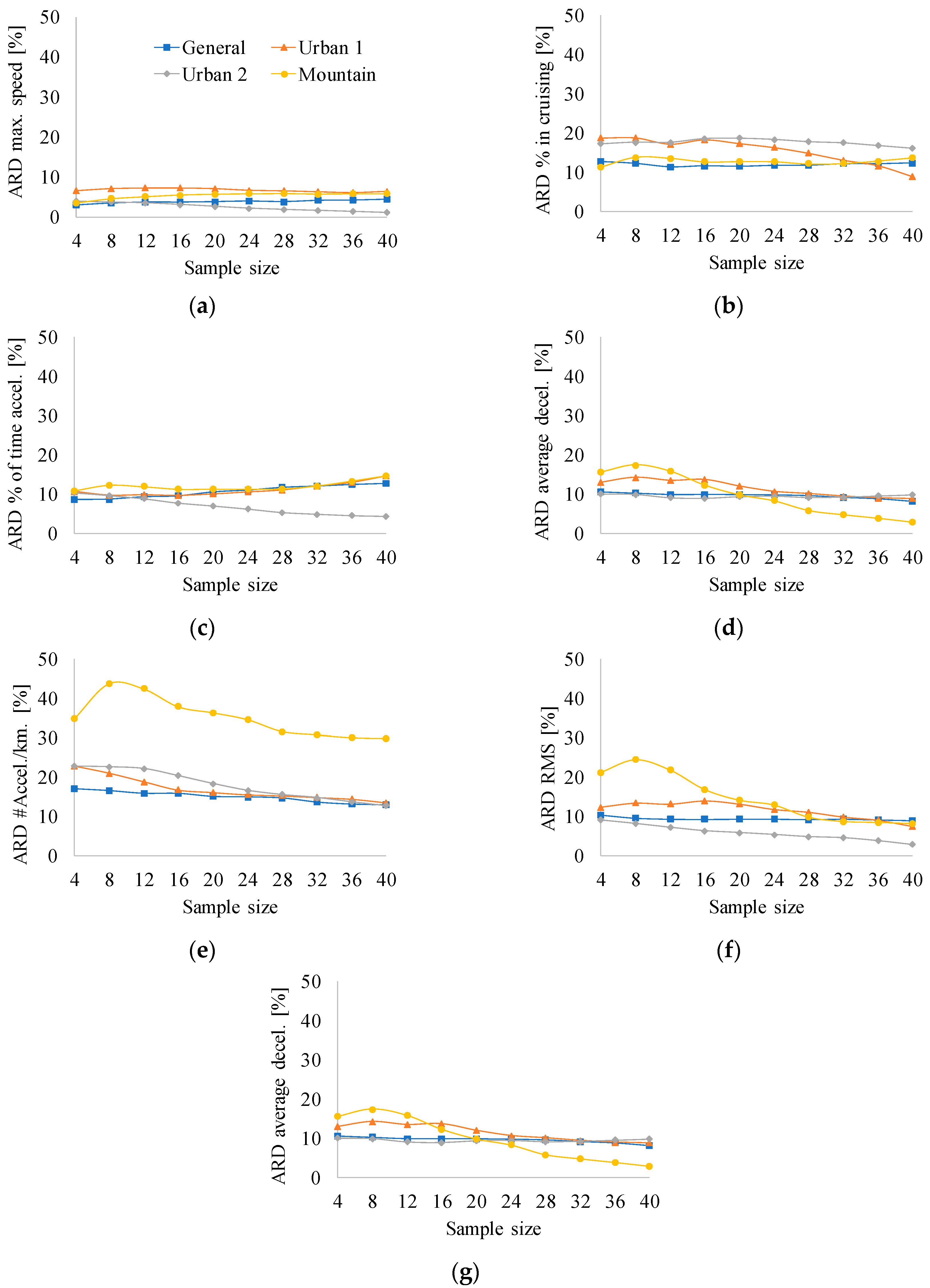
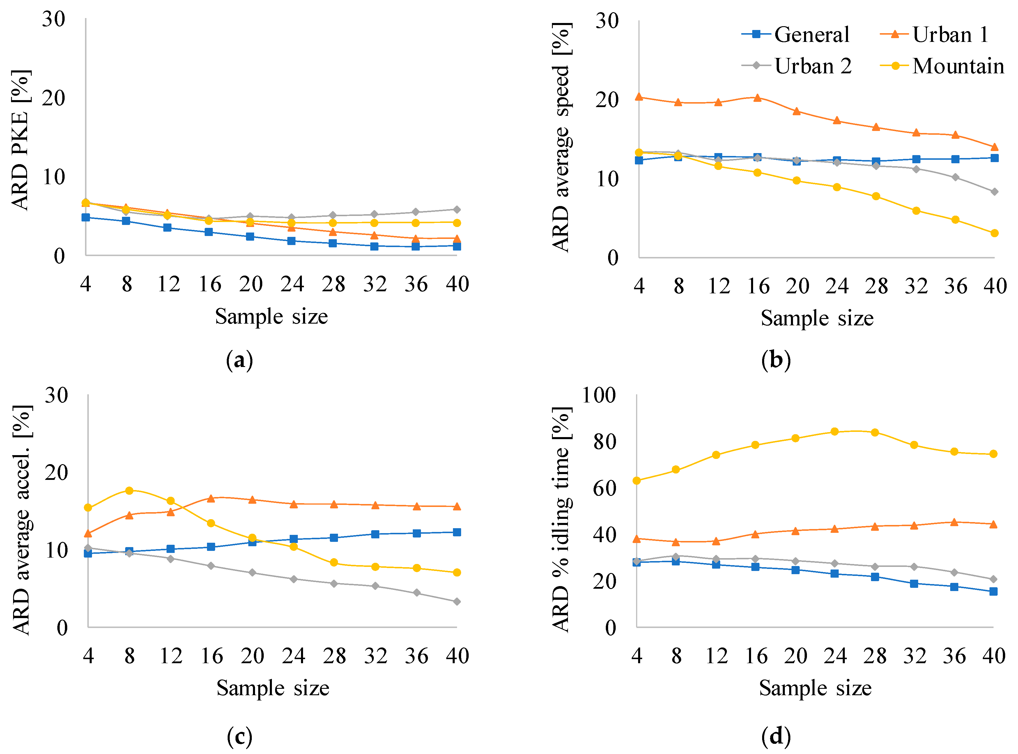
• We evaluated the relative differences of the CPs of the selected fuel-based-DC with respect to the average CPs of the trips sampled. We repeated the process for a large number of subsets of sampled trips.

Next, we describe the details of each of these tasks.

2.1. Regions of Study

With the goal of providing generality to our work, we looked for regions with different topographies, located at high altitudes, featuring well-maintained roads and with different level of services (LoS).

We selected regions open to private companies offering regular passenger and cargo transit services. We considered four cases (

Table 1. Characteristics of the roads considered in this work.

Parameter	Unit	Urban 1	Urban 2	Uphill	Mountain	General
Location	-	Mexico City	TOL	-	-	TOL-MEX
Facility	-	Local roadway	Arterial	Freeway	Freeway	Combined
Level of traffic	-	High	Medium	Medium	Low-Medium	Low-High
LoS *	-	F	E	C	C-B	B-F
Speed limit	km/h	60	60	80	110	60–110
Number of lanes	-	3	3	4	4	3–4
Length	km	11.5	18.8	16.1	41.3	71.6
Ave road grade	%	1.4	1.8	6.1	5.6	4.0
Max road grade	%	5.2	9.0	15.0	15.0	15.0
Min altitude	m.a.s.l.	2255	2611	2255	2233	2233
Max altitude	m.a.s.l.	2258	2637	3313	3313	3313

* LoS: Level of service. LoS is the level of quality of a traffic facility and represents a range of operating conditions, generally in terms of service measures such as speed and travel time, freedom to maneuver, traffic interruptions, and comfort and convenience. Classification was done according to the US Highway capacity manual [25].

).

• Urban 1, which corresponds to a flat, densely populated region. We arbitrarily selected a set of roads covering 11.5 km inside Mexico City (2255 m above sea level (m.a.s.l.)). These roads are characterized by highly congested traffic (i.e., LoS E or F).
• Urban 2, which corresponds to a flat region located on the outskirts of an urban region. We selected an 18.8 km-long road located on the outskirts of Toluca City (2611 m.a.s.l.), which has four lanes with a medium traffic flow (i.e., LoS E).
• Mountain, whose topography includes significant altitude changes (>500 m). We selected a 41.3 km-long highway connecting the cities of Toluca and Mexico. This region starts at 2255 m.a.s.l., ascends to 3313 m.a.s.l., and then it descends to 2611 m.a.s.l. with a maximum road grade of approximately 15%. It has four lanes with high traffic (~33,632 daily vehicles, i.e., LoS C).
• General, which is a combination of the previous cases. The selected set of regions spans 71.6 km, with altitude variations from 2233 to 3313 m.a.s.l. and a maximum road grade of approximately 15%. This set of regions has both urban and suburban sections.

2.2. Vehicles

We looked for vehicles of the same technology with similar maintenance conditions, aiming to eliminate their effects on our study. Our collaborating company has a fleet of 680 passenger buses, with 28 express buses that operate in the regions described previously, making no intermediate stops to pick up or drop off passengers. The fleet of buses used in this study were made between 2012 and 2014. They use diesel-fueled engines (Cummins ISM 425) that deliver 425 HP and 2102 Nm. These busses have a capacity of 49 passengers and their gross vehicle weight is 13,850 kg. They are 3.6 m tall, 12.85 m long and 2.6 m wide. They exhibit an aerodynamic drag coefficient of 0.64 and a rolling resistance coefficient of 0.006 [26].

2.3. Instrumentation

The measurement of instantaneous FC is essential to our work. Automotive diesel technology controls the amount of fuel injected into the engine combustion chamber by controlling the fuel injection time. This variable is available in the engine control unit (ECU) and can be read via the on-board diagnosis (OBD) system. We used the OBD interface provided by the engine manufacturer to read, report and store the instantaneous engine FC at a 1 Hz sampling period. We verified the accuracy of the data obtained using this interface by comparing the FC obtained via OBD with results obtained using an external graduated tank, which is the standard procedure to determine vehicle FC [27,28]. Based on the determination coefficient (R² > 0.9) and calibration slopes (m = 1.06) obtained in a correlation analysis between the results obtained by these two methods, we concluded that the determination of fuel consumption via OBD produces results comparable to the ones obtained using the calibrated tank.

High precision GPSs (

Table 2. Technical characteristics of the instruments used in this study

Variable	Instrument/Trademark	Technical Characteristics
Position: latitude, longitude and altitude Speed and time	GPS/Garmin 16x	Position: 3–5 m, 95% typical Frequency: 1 Hz Speed: 0.05 m/s RMS steady state PPS time: 1 microsecond at rising edge of PPS pulse
Instantaneous fuel consumption	-	Estimated through the injection time Reported by ECU through OBD2

GPS: global position system; OBD2: on-board diagnostic system, second generation; ECU: engine control unit.

) were used to monitor position, altitude and speed of the vehicles as functions of time. Algorithms were developed to identify events where data were missing or had atypical values. Trips with less than 90% of data availability were disregarded. It was observed that the speed values reported by GPS were equivalent to those reported by the OBD system. The GPS altitude was compared with manual measurements of altimetry. An additional algorithm was developed to correct frequent errors in the GPS-reported altitude.

2.4. Data Collection

Four monitoring campaigns were carried out to obtain real on-road driving data. One monitoring campaign was performed per region as described in Table 1 (Urban 1, Urban 2, Mountain and General). Each region was measured in both directions using the instrumented buses described in the previous section. Buses were driven by the company’s regular drivers, and the buses were in service while we monitored the driving variables (speed and time) along with altitude and instantaneous FC at a frequency of 1 Hz, minimizing any disruption to regular vehicle operation. The monitoring campaigns included trips during different hours of the day, different days of the week, including weekends, and different seasons of the year. The data quality was verified. Trips with less than 90% of data availability were disregarded. After QA/QC analyses, 46 trips per region were left with simultaneous measurements of position, altitude, speed, and FC.

2.5. Assessment Methodology

To gain generality in our conclusions, we studied the effects of the number of trips sampled on our results by randomly selecting sub-samples of trips out of the 46 trips sampled per region. The size of the sub-samples varied between 4 and 40. For each sample size, we repeated the sub-sampling process 1000 times.

At each instance, we applied the fuel-based method. This is, we selected the trip j with the FC closest to the mean value for the FC of the sub-sample ($\overline{FC}$ in Equation (1)):

$$DC=Arg\left\{mi{n}_j\left|F{C}_j-\left(\overline{FC}\right)\right|\right\}$$

(1)

Statistically speaking, the average FC calculated from the sub-sample is an estimation of the true mean FC of the whole population of busses monitored in each region. As we will show later, the FC in every region followed a normal distribution (Figure 1) and therefore, the average value of the sub-sample is a good descriptor the true mean FC.

We hypothesized that by using the fuel-based method, implicitly, the obtained DC represents the driving patterns. I.e., the characteristic parameter i of the obtained local DC (CP_i^*) will be close to the average value obtained for that parameter from the sampled trips (${\overline{CP}}_i$). To test this hypothesis, we calculated the relative difference of CP_i^* with respect to ${\overline{CP}}_i$ at each iteration of the analysis described previously. Then, for each of the CP_i listed in

Table 3. Characteristic parameters (CPs) that describe the driving patterns followed by drivers during the monitoring campaigns at every region considered in this study.

	CP	Unit	Regions
			General			Urban 1			Urban 2			Mountain			HD UDDS
Dynamics	RMS	m/s2	0.39	±	0.01	0.41	±	0.02	0.43	±	0.02	0.35	±	0.02	0.47
	PKE	m/s2	0.25	±	0.01	0.34	±	0.02	0.34	±	0.02	0.19	±	0.01	0.27
	Accelerations per kilometre	km−1	7.9	±	0.8	11.8	±	2.5	8.5	±	0.8	6.6	±	0.8	10.7
Operation modes	Percentage idling	%	14.7	±	1.7	21.9	±	3.9	20.3	±	2.7	2.6	±	0.9	33.3
	Percentage acceleration	%	27.6	±	1.0	27.6	±	1.9	28.8	±	1.7	27.3	±	1.4	22.2
	Percentage deceleration	%	24.6	±	0.8	25.9	±	1.5	25.0	±	1.7	24.3	±	1.2	20.2
	Percentage cruising	%	33.1	±	1.5	24.6	±	1.8	25.9	±	1.8	45.7	±	2.6	24.3
Speed	Average speed	m/s	10.5	±	0.7	6.8	±	0.9	7.9	±	0.7	16.6	±	1.2	8.4
	SD speed	m/s	9.0	±	0.2	6.2	±	0.5	7.3	±	0.2	8.6	±	0.6	8.9
	Maximum speed	m/s	28.6	±	0.5	21.9	±	1.0	26.5	±	0.6	28.5	±	0.5	25.9
Acceleration	Average acceleration	m/s2	0.43	±	0.01	0.46	±	0.01	0.46	±	0.02	0.37	±	0.01	0.57
	Average deceleration	m/s2	−0.48	±	0.01	−0.49	±	0.02	−0.52	±	0.02	−0.43	±	0.02	−0.64
	SD acceleration	m/s2	0.24	±	0.01	0.25	±	0.01	0.25	±	0.01	0.21	±	0.01	0.37
	SD deceleration	m/s2	0.35	±	0.02	0.35	±	0.01	0.39	±	0.02	0.31	±	0.02	0.40
	Maximum acceleration	m/s2	1.51	±	0.07	1.37	±	0.08	1.41	±	0.06	1.31	±	0.08	1.96
	Maximum deceleration	m/s2	−2.29	±	0.15	−1.96	±	0.10	−2.13	±	0.14	−2.05	±	0.16	−2.07

SD: standard deviation, RMS: root mean square, HD UDDS: heavy duty urban dynamometer driving schedule, PKE: positive kinetic energy. $PKE=\frac{1}{L}{\displaystyle \sum }_{i=2}^n{v}_i{}^2-v_{i-1}{}^2 ,\mathrm{for} v_i>v_{i-1}, \mathrm{otherwise}PKE=0$. L is the distance traveled and v_i is vehicle speed at second i.

, we reported the average relative differences (ARD_i) obtained for each sample size after n =1000 iterations (Equation (2)):

$$AR{D}_i={{\displaystyle \sum }}_{j=1}^n\frac{\left(C{P}_i{}^{*}-\overline{C{P}_i}\right)}{n\overline{C{P}_i}}$$

(2)

Additionally, we used the quality of fit (QoF) metric (Equation (3)), [29] to evaluate the degree of similarity of the speed-acceleration probability distribution (SAPD) of the selected fuel-based DC to the SAPD of the subset of sampled trips. In Equation (3), P_i,j^* is the probability that the vehicle travels within the bin i, j of speeds and accelerations, in the states matrix obtained for the selected DC. $\overline{P_{ij}}$ is the corresponding average probability obtained for the sub-sample of trips. This metric is independent of the number of bins used in the discretization of the speed and acceleration ranges and has a maximum value of 2:

$$QoF={\displaystyle \sum }_{i=1}^n{\displaystyle \sum }_{j=1}^m{(P_{i,j}^{*}-\overline{P_{ij}})}^2$$

(3)

3. Results and Discussion

3.1. Description of Driving Patterns

As stated before, driving patterns are described by CPs but currently it is unknown which set of CPs fully describe them. It is feasible that some CPs could be no good descriptors of the driving pattern and that some CPs could be redundant (linearly dependent of others). Furthermore, it is also feasible that additional CPs or metrics are needed to fully describe those patterns. This could be the case of driving patterns in mountain regions where metrics that directly influence FC, such as average road grade, should be added to the set of CPs.

As the primary objective of this work is not to determinate the CPs or metrics required to fully describe a driving pattern, we selected the CPs most used in the literature. Table 3 lists those CPs. It also includes their average values obtained from the 46 trips sampled during the monitoring campaign and their confidence intervals with confidence level of 95%. Additionally, for comparison purposes, we included the values of these CPs for the heavy duty urban dynamometer driving schedule (HD UDDS). As expected, the resulting values depend on the local conditions and therefore their inter-comparison is meaningless.

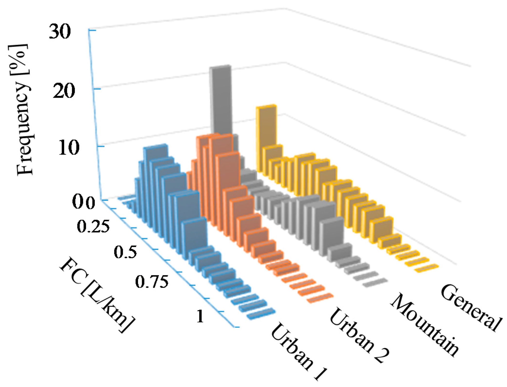
3.2. The SFC Distribution

As described in Section 2.5, we first needed a criterion to describe the mean FC of the subset of sampled trips. Classical statistics recommends the use of average values for this purpose, but this parameter is limited to cases in which the data exhibit a normal frequency distribution.

Figure 1 shows the FC frequency distribution obtained for all the buses in the regions considered in this study. We performed Anderson-Darling goodness-of-fit tests to evaluate if the FC of the vehicles were normally distributed and found p-values greater than 0.12 for all regions. This result indicates that, with a probability of 95%, those distributions fit a normal distribution. The 16 t buses monitored in this study showed a FC of 0.41 ± 0.04 L/km in the region with high traffic (Urban 1), and of 0.37 ± 0.02 L/km in the region with medium level of vehicular traffic (Urban 2), which represent an FC with relative differences of less than 11% with respect to the combined region (0.37 ± 0.03 L/km). Unexpectedly, the minimum FC was obtained in mountainous regions with an average of 0.36 ± 0.04 L/km. For the purposes of possible future comparisons, these vehicles showed an SFC of 0.62 ± 0.03 L/km when they were travelling uphill on an average road grade of 6.1% and at an average speed of 66.6 km/h.

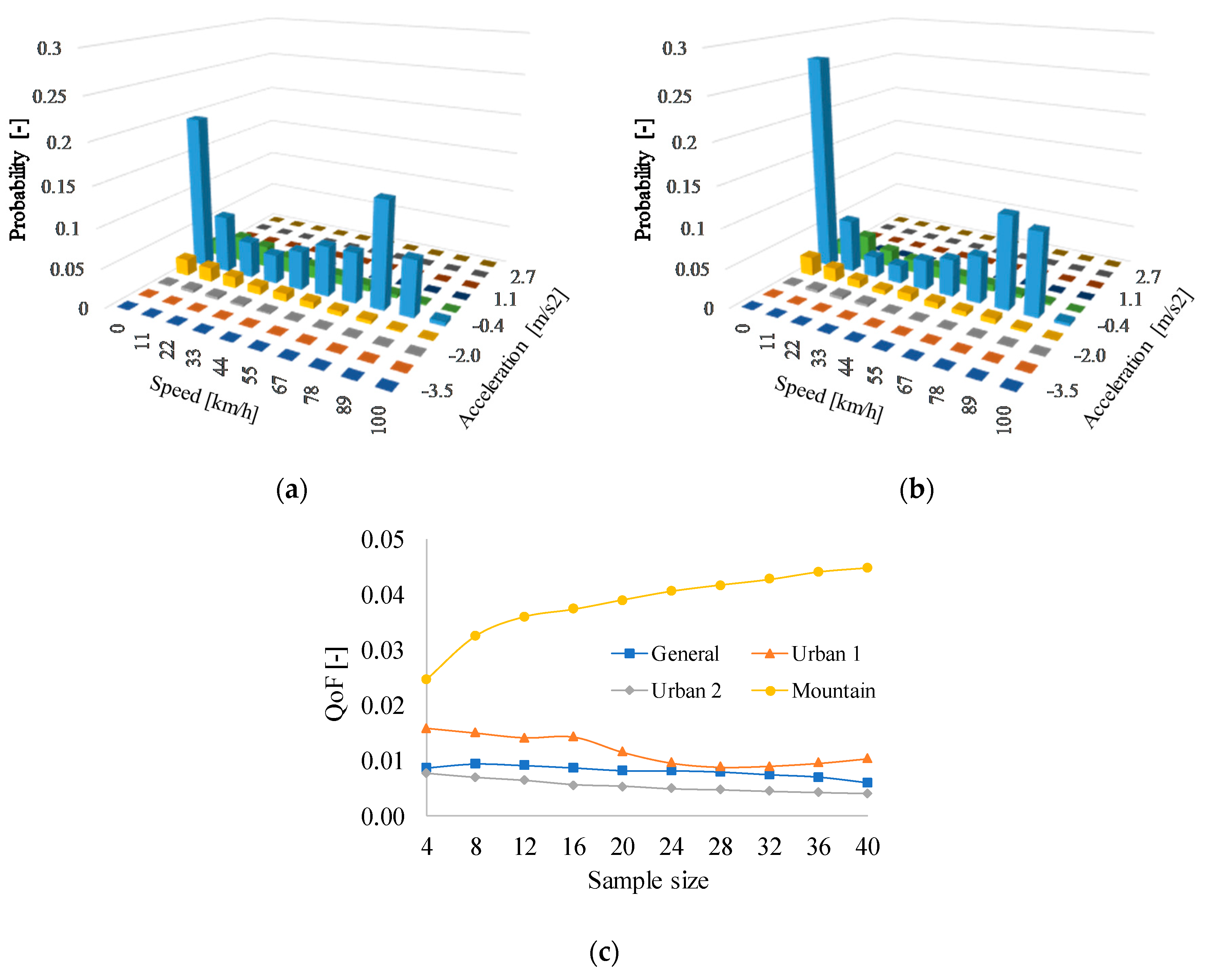
3.3. Similitude of CPs and SAFDs

As stated before, we aimed to demonstrate that the fuel-based DC exhibit CPs (CP_i^*) close to the respective average CPs of the sampled trips (${\overline{CP}}_i$). Figure 2 shows the average relative differences (ARD_i), as function of sample size, for some common CPs used to describe driving patterns.

Figure 2a shows the ARDs for the case of positive kinetic energy (PKE), which is a CP that directly influences FC. It shows that for all the regions, these differences are on average <10% after considering 1000 potential cases. These ARDs tend to decrease with the number of trips sampled, reaching a value of approximately 1.0% for a sample size of 40.

The same behavior was observed for the case of average speed (Figure 2b) and average acceleration (Figure 2c) but the ARDs were <20%. These percentage of relative differences continue being small, especially considering they could range from cero to infinity and that they were obtained after considering 1000 possible cases.

Figure 2d shows the results of the ARDs for case of the percentage of idling time. It shows that the ARDs exhibit the same behavior as in previous cases but these differences on average are smaller than 40%, except for the mountain region. In this last region, the obtained ARD can be high (<80%), and it does not always decrease with an increase in the number of trips sampled. Table 3 shows that in this region, the percentage of idling time is small (2.6%) and therefore small absolute variations on idling time make the relative difference (ARDs) high. Idling time is a CP that weakly influence FC. It could be considered as an external factor or a non-related-human-factor, in consideration that when travelling, drivers naturally do not stop unless external factors force them to stop.

Other CPs are shown in Appendix A. For all CPs, the ARDs obtained are smaller than 20% except for the mountain region that in some cases reached ARDs of up to 40%.

Several authors also use the speed-acceleration probability distribution (SAPD) as an alternative to describe DCs [4,11,17]. The SAPD can be thought of as a two-dimensional CP. We evaluated the level of closeness of the obtained SAPD for the selected fuel-based DC and the SAPD for the trips sampled, following the methodology described in Section 2.5.

Figure 3 shows (as an example) the SAPD obtained for a sample of 10 trips in the Urban 1 region (Figure 3a) and the corresponding SAPD obtained for the obtained fuel-based DC (Figure 3b). Qualitatively, they look similar. We used the quality of fit metric (QoF, Equation (3)) to quantify the level of similarity. Figure 3c shows the QoF metric as a function of the numbers of trips sampled. It shows that the QoF in all cases is smaller than 0.05, and those differences in probabilities expressed by the QoF tend to decrease with sample size, except for the case of the Mountain region. These values are negligible compared with the maximum value that this metric can assume (QoF = 2). Additionally, these values are also comparable to the ones found by Günther et al. [29] for the case of two similar DCs (QoF~10⁻³). These observations confirm that the SAPD of the DC with the FC closest to the average measured FC of the sample is similar to the SAPD of the sampled trips.

These results confirm that by using FC as the criterion of representativeness for a DC, the fuel consumption, CPs and SAPD of the fuel-based DCs are close to the measured fuel consumption, CPs and SAPD in flat regions.

Our experimental result for ARDs and QoFs also suggest that samples of 10 to 20 trips are sufficient to describe the driving patterns in flat regions. However, we highlight that this result is valid for a single vehicle technology used with a single purpose, which is the scope of our work reported in this manuscript.

4. Conclusions

Large differences currently observed in fuel consumption (FC) with respect to the FC reported by manufactures are mainly due to the lack of representativeness of the local driven conditions contained in the type-approval driving cycles used by manufactures during the introduction process of new vehicle technologies in the market.

A driving cycle (DC) represents the typical driving pattern of a given region when its characteristic parameters (CP*s) exhibit similar values to the average CPs that describe the driving pattern in that region. Current alternatives to construct DC are repeatable but no reproducible, and there is no evidence that the resulting DC reproduce real vehicle fuel consumption (FC).

To address these two issues we followed the suggestion of several author of using FC as criteria to construct those DCs. We hypothesized that by re-defining a DC as the time series of speeds that when followed by a vehicle, its FC is similar to the average FC of all vehicles of similar technology operating in the same region, implicitly, the resulting DC describes the driving patterns in that region. Thus, we proposed to sample a large set of time series of speeds (trips), simultaneously with vehicle FC. Then, the trip with the FC closest to the average value of FC of the entire population of trips sampled is selected as the representative DC.

To demonstrate this hypothesis, we simultaneously monitored at a frequency of 1 Hz, for 8 months, the location, speed, altitude, and FC of a fleet of 15 vehicles of similar technology operating under normal conditions of use, in four regions of diverse topography and on roads of diverse level of service (LoS). We observed the average relative difference (ARD) between the CP*s of the selected fuel-based DC and the CPs of the monitored driving pattern.

For the flat regions considered in this study, we obtained differences smaller than 15% for the CPs related to speed and acceleration that are directly influenced by the driver´s decisions, such as average speed, positive kinetic energy, and average positive acceleration. We also observed that the speed-acceleration probability distribution (SAPD) of the selected fuel-based DC is similar to the SAPD of the sampled trips (QoF ≤ 0.05). Furthermore, the level of similarity between CPs and SAPDs increased with the number of trips sampled.

These results confirmed our hypothesis. However, the percentage of idling time that could be considered an external factor (not a descriptor of driver patterns) showed the highest relative differences (up to 80% for the case of mountain regions). These differences could still be considered acceptable taking into consideration that: (1) this variable range from 0 to infinity; (2) we obtained those results after considering 1000 possible cases and (3) for the case of the mountain region the time spent by vehicles idling was short and therefore any small absolute difference has a large value when expressed as relative difference. Nevertheless, additional work is required to confirm the results described in this manuscript for several other vehicles technologies, and to establish the methodology to implement the resulting DC in a chassis dynamometer, specially, for the case of mountain regions.

References

1. Tietge, U.; Mock, P.; Franco, V.; Zacharof, N. From laboratory to road: Modeling the divergence between official and real-world fuel consumption and CO2 emission values in the German passenger car market for the years 2001–2014. Energy Policy 2017, 103, 212–222. [Google Scholar] [CrossRef]
2. Brundell-Freij, K.; Ericsson, E. Influence of street characteristics, driver category and car performance on urban driving patterns. Transp. Res. Part D Transp. Environ. 2005, 10, 213–229. [Google Scholar] [CrossRef]
3. Ericsson, E. Independent driving pattern factors and their influence on fuel use and exhaust emission factors. Transp. Res. Part D Transp. Environ. 2001, 6, 325–345. [Google Scholar] [CrossRef]
4. Tong, H.Y.; Hung, W.T. A framework for developing driving cycles with on-road driving data. Transp. Rev. 2010, 30, 589–615. [Google Scholar] [CrossRef]
5. Achour, H.; Olabi, A.G. Driving cycle developments and their impacts on energy consumption of transportation. J. Clean. Prod. 2016, 112, 1778–1788. [Google Scholar] [CrossRef]
6. Ashtari, A.; Bibeau, E.; Shahidinejad, S.; Ashtari, A. Using Large Driving Record Samples and a Stochastic Approach for Real-World Driving Cycle Construction: Winnipeg Driving Cycle. Transp. Sci. 2014, 48, 170–183. [Google Scholar] [CrossRef]
7. Giakoumis, E.G. Driving and Engine Cycles; Springer: Cham, Switzerland, 2017; p. 422. ISBN 978-3-319-49033-5. [Google Scholar]
8. Huang, D.; Xie, H.; Ma, H.; Sun, Q. Driving cycle prediction model based on bus route features. Transp. Res. Part D 2017, 54, 99–113. [Google Scholar] [CrossRef]
9. Ko, J.; Jin, D.; Jang, W.; Myung, C.L.; Kwon, S.; Park, S. Comparative investigation of NOxemission characteristics from a Euro 6-compliant diesel passenger car over the NEDC and WLTC at various ambient temperatures. Appl. Energy 2017, 187, 652–662. [Google Scholar] [CrossRef]
10. Barlow, T.; Latham, S.; Mccrae, I.; Boulter, P. A Reference Book of Driving Cycles for Use in the Measurement of Road Vehicle Emissions; TRL Published Project Report; Transport Research Laboratory: Wokingham, UK, 2009. [Google Scholar]
11. Brady, J.; Mahony, M.O. Development of a driving cycle to evaluate the energy economy of electric vehicles in urban areas. Appl. Energy 2016, 177, 165–178. [Google Scholar] [CrossRef]
12. Tamsanya, N.; Chungpaibulpatana, S. Influence of driving cycles on exhaust emissions and fuel consumption of gasoline passenger car in Bangkok. J. Environ. Sci. 2009, 21, 604–611. [Google Scholar] [CrossRef]
13. Pavlovic, J.; Ciuffo, B.; Fontaras, G.; Valverde, V.; Marotta, A. How much difference in type-approval CO2 emissions from passenger cars in Europe can be expected from changing to the new test procedure (NEDC vs. WLTP)? Transp. Res. Part A Policy Pract. 2018, 111, 136–147. [Google Scholar] [CrossRef]
14. Tutuianu, M.; Bonnel, P.; Ciuffo, B.; Haniu, T.; Ichikawa, N.; Marotta, A.; Pavlovic, J.; Steven, H. Development of the World-wide harmonized Light duty Test Cycle (WLTC) and a possible pathway for its introduction in the European legislation. Transp. Res. Part D Transp. Environ. 2015, 40, 61–75. [Google Scholar] [CrossRef]
15. Ho, S.; Wong, Y.; Chang, V.W. Developing Singapore Driving Cycle for passenger cars to estimate fuel consumption and vehicular emissions. Atmos. Environ. 2014, 97, 353–362. [Google Scholar] [CrossRef]
16. Shi, Q.; Zheng, Y.; Wang, R.; Li, Y. The study of a new method of driving cycles construction. Procedia Eng. 2011, 16, 79–87. [Google Scholar] [CrossRef]
17. Hung, W.T. Development of a practical driving cycle construction methodology: A case study in Hong Kong. Transp. Res. Part D 2007, 12, 115–128. [Google Scholar] [CrossRef]
18. Bishop, J.D.K.K.; Axon, C.J.; Mcculloch, M.D. A robust, data-driven methodology for real-world driving cycle development. Transp. Res. Part D Transp. Environ. 2012, 17, 389–397. [Google Scholar] [CrossRef]
19. Zhang, X.; Zhao, D.-J.; Shen, J.-M. Energy Procedia A Synthesis of Methodologies and Practices for Developing Driving Cycles. Energy Procedia 2012, 16, 1868–1873. [Google Scholar] [CrossRef]
20. Gong, Q.; Midlam-Mohler, S.; Marano, V.; Rizzoni, G. An Iterative Markov Chain Approach for Generating Vehicle Driving Cycles. SAE Int. 2011, 4, 1035–1045. [Google Scholar] [CrossRef]
21. Lin, J.; Niemeier, D.A. An exploratory analysis comparing a stochastic driving cycle to California’s regulatory cycle. Atmos. Environ. 2002, 36, 5759–5770. [Google Scholar] [CrossRef]
22. Shi, S.; Lin, N.; Zhang, Y.; Cheng, J.; Huang, C.; Liu, L.; Lu, B. Research on Markov property analysis of driving cycles and its application. Transp. Res. Part D 2016, 47, 171–181. [Google Scholar] [CrossRef]
23. Huertas, J.I.I.; Díaz, J.; Cordero, D.; Cedillo, K. A new methodology to determine typical driving cycles for the design of vehicles power trains. Int. J. Interact. Des. Manuf. 2018, 12, 319–326. [Google Scholar] [CrossRef]
24. Liu, J.; Wang, X.; Khattak, A. Customizing driving cycles to support vehicle purchase and use decisions: Fuel economy estimation for alternative fuel vehicle users. Transp. Res. Part C Emerg. Technol. 2016, 67, 280–298. [Google Scholar] [CrossRef]
25. National Academies of Science. Highway Capacity Manual 2010; National Academies of Science: Washington, DC, USA, 2010; ISBN 0738-6826. [Google Scholar]
26. Huertas, J.I.; Álvarez Coello, G.A. Accuracy and precision of the drag and rolling resistance coefficients obtained by on road coast down tests. In Proceedings of the International Conference on Industrial Engineering and Operations Management, Bogota, Colombia, 25–26 October 2017. [Google Scholar]
27. Pīrs, V.; Jesko, Ž.; Lāceklis-Bertmanis, J. Determination methods of fuel consumption in laboratory conditions. Eng. Rural Dev. 2008, 1, 154–159. [Google Scholar]
28. SAE International. J1321: Fuel Consumption Test Procedure—Type II; SAE International: Warrendale, PA, USA, 2012. [Google Scholar]
29. Günther, R.; Wenzel, T.; Wegner, M.; Rettig, R. Big data driven dynamic driving cycle development for busses in urban public transportation. Transp. Res. Part D 2017, 51, 276–289. [Google Scholar] [CrossRef]
Figure 1. Frequency distribution of the FCs measured of all trips considered in this study.
Energies 11 03064 g001
Figure 2. Average relative differences (ARD) of common characteristic parameters (CPs) used to describe driving cycles (DC) as a function of the number of trips sampled and the type of regions used in this study. (a) positive kinetic energy (PKE); (b) average speed; (c) percentage of time with positive acceleration; (d) percentage of idling time.
Energies 11 03064 g002
Figure 3. Comparison of the speed-acceleration probability distribution (SAPD) obtained for: (a) The sampled trips and; (b) The SFC closest to the average measured SFC of the sampled trips; (c) QoF as a function of the number of sampled trips.
Energies 11 03064 g003