An Online Data-Driven Model Identification and Adaptive State of Charge Estimation Approach for Lithium-ion-Batteries Using the Lagrange Multiplier Method

Abstract

Reliable and accurate state of charge (SOC) monitoring is the most crucial part in the design of an electric vehicle (EV) battery management system (BMS). The lithium ion battery (LIB) is a highly complex electrochemical system, which performance changes with age. Therefore, measuring the SOC of a battery is a very complex and tedious process. This paper presents an online data-driven battery model identification method, where the battery parameters are updated using the Lagrange multiplier method. A battery model with unknown battery parameters was formulated in such a way that the terminal voltage at an instant time step is a linear combination of the voltages and load current. A cost function was defined to determine the optimal values of the unknown parameters with different data points measured experimentally. The constraints were added in the modified cost function using Lagrange multiplier method and the optimal value of update vector was determined using the gradient approach. An adaptive open circuit voltage (OCV) and SOC estimator was designed for the LIB. The experimental results showed that the proposed estimator is quite accurate and robust. The proposed method effectively tracks the time-varying parameters of a battery with high accuracy. During the SOC estimation, the maximum noted error was 1.28%. The convergence speed of the proposed method was only 81 s with a deliberate 100% initial error. Owing to the high accuracy and robustness, the proposed method can be used in the design of a BMS for real time applications.

1. Introduction

Rechargeable batteries are becoming the energy tanks and power sources for a wide range of applications, ranging from low power cellphones and notebooks to large high-power submarine, aircraft, satellite, smart grid, electric vehicle (EV), and hybrid electric vehicle (HEV) applications [1,2,3,4]. Lithium-ion batteries are becoming increasingly popular in many applications owing to their high energy/power density, environmental friendliness, low self-discharge rate, and long lifetime [5,6,7]. An effective and robust battery management system (BMS) is needed to enhance the lifetime, efficiency, and reliability of lithium ion batteries. The main function of BMS is to monitor and measure the state of health (SOH), state of power, and specifically the state of charge (SOC) [8,9,10]. The SOC is defined as the ratio of the present capacity to the total capacity [11]. The SOC of energy storage systems (ESSs) is the key state variable to monitor and to avoid over charge/discharge and regulating energy dispatch [12]. Despite the importance, the precise and reliable determination of the SOC is still a bottleneck for researchers because the SOC is an internal state of a battery and a battery has very nonlinear and time-variable characteristics. Therefore, it cannot be measured directly using any physical sensor.

In the past, an assortment of techniques have been presented to estimate or determine the SOC of battery packs or cells [13,14,15,16,17,18,19,20]. Every technique has its own merits and demerits. The methods of SOC estimation can be divided into two main categories: (i) non-model-based methods and (ii) model-based methods. Non-model-based methodologies for estimating the SOC are Ampere-hour counting (Coulomb counting) and the open circuit voltage (OCV) methods. The Ampere-hour counting method is quite simple, reliable and easily implementable using very low-priced current sensors [13,14,15,16,17,18,19,20,21]. This method requires a very precise initial estimate of the SOC, which is almost impossible to measure in real applications. In addition, the lack of a feedback mechanism and the effect of noise on the current sensor are also other demerits. The OCV method is a very simple and straightforward method with very high accuracy [14,15,16,17,18,19,20,21,22]. On the other hand, it requires a sufficient relaxing time to measure the OCV information accurately and the battery should be cut off or left to stand for some time until the output voltage of the battery reaches the OCV. Therefore, this method is impractical for use in real-time applications. Owing to the good adaptability and high accuracy, model-based approaches are the most well-known in the design and analysis of a BMS. The model-based SOC estimation method can be divided easily into three main categories: physical models [23,24], electrochemical models [25,26], and equivalent circuit models (ECMs) [27,28,29,30,31]. The physical models are designed only for a specific battery factor, such as the temperature model [23] and cycle life model [24]. Nevertheless, complete battery operation cannot be described using a single specific factor. The electro-chemical models have very high accuracy, but complex mathematical equations make the SOC estimation process arduous. Among these battery models, ECMs are most preferred, intuitive, simple and realistic than the others [14,15,16,17,18,19,20,21]. In ECMs, the dynamic behavior of a battery is represented using simple electrical components, such as resistors and capacitors [27,28,29,30,31,32]. In general, this approach resulting in a system of nonlinear ordinary differential equations or their discrete form for the states variables (internal voltages, SOC and temperature). ECMs can be treated with the methods of mathematical control, filter and system theory. ECMs can be divided further into three sub models: Thevenin-based electrical model [29,30], impedance-based electrical model [31], and runtime-based electrical model [32]. Every model has its own merits and demerits. The Thevenin-based model is used most commonly because of its simplicity, low computational complexity, and reasonable accuracy [14,15,16,17,18,19,20,21]. For precise estimations of any state of a battery, the accuracy and complexity of the battery model are the most important factors.

Among these models, the ECMs are most popular for estimating the SOC. Several adaptive filters have been merged with an ECM to estimate the state of batteries, which are usually classified into two main types: offline method and online method [33]. The offline method uses archived data to determine the battery parameters, but the online method has been applied to solve the battery model parameters in real time measurements. Several researchers have presented different offline method logics to calculate the model’s parameters. Hu et al. [34] constructed an adaptive Luenberger observer to estimate the SOC. Plett [20] proposed the use of an extended Kalman filter (EKF) to estimate the SOC. On the other hand, the EKF was quite unstable during linearization. Zou et al. [35] used an unscented Kalman filter (UKF) to design an estimator for SOC and a SOH estimation using lower order battery models. The overall performance of Kalman filters abruptly decreased in the presence of non-Gaussian noise. Gao et al. [36] introduced the idea that a particle filter (PF) can deal with highly non-linear and non-Gaussian models. PF is based on Monte-Carlo methods to estimate the posterior distribution. To estimate the SOC, the sliding mode observer [37] and H-infinity observer [38] have also been reported. These methods cannot achieve high precision because they are based on fixed battery parameters. The battery states are quite sensitive and can be affected by slight changes in temperature, discharge/charges current rate, and battery aging [39]. These environmental and system parameters are independent of the user control. This causes uncertainty in a battery model parameter determination and may result in an unavoidable perturbation in a SOC estimation. Therefore, online battery modelling has attracted considerable research attention because it not only estimates the SOC precisely under different conditions and aging levels, is but it is also useful for battery efficiency enhancement. Salkind et al. [40] used impedance spectroscopy and fuzzy logic to propose a SOC estimator. Chin et al. [41] used an adaptive online sequential extreme learning machine (AOS-ELM) to estimate SOC at different temperature. In these techniques, battery is considered as a “black box” and machine learning techniques were used to analyze the data. These techniques are highly efficient but require high storage and computational time. Piao et al. [42] proposed statistical methods for the online model identification of a battery. This method showed reasonable accuracy in a SOC estimation of a Ni-MH battery, but the SOC of a lithium ion battery cannot be estimated accurately using this method because a lithium ion battery has a flat OCV plateau. In recent years, a recursive least squares (RLS) method used widely for updating the battery parameter in real time with the conjunction of different adapting algorithms was used to estimate the SOC [30,33,43,44]. Hu et al. [45] proposed the using a dual extended Kalman filter (DUKF) to estimate the SOC in real time. A dual nonlinear predictive filter (DNPF) was also used to estimate the SOC and battery parameters [46]. Kang et al. [47] presented the black box approach. This technique does not require any battery dynamics, and the accuracy of the SOC depends mainly on the quality and quantity of data. Therefore, it requires higher computational power and storage. Although so many efforts have been made for online SOC estimations, the stability, robustness and low computational cost is still a challenging task.

This paper proposes a data-driven online model identification method. The Lagrange multiplier method was used to identify the battery model parameters in real time using the battery voltage and current. The first order RC (resistor and capacitor) battery model was taken to manage the tradeoff between the complexity and accuracy. The adaptive estimators were designed to estimate the OCV and SOC of LIB. Different experiments were performed to validate the robustness and accuracy of the proposed technique.

The remainder of the paper is organized as follows: Section 2 presents the battery modeling and data driven battery parameters estimation technique. The adaptive OCV and SOC estimator are described in Section 3. Details of the experimental setup are presented in Section 4. The results to validate the proposed technique are discussed in Section 5. The conclusions are summarized in the final section.

2. Battery Modelling and Parameter Estimation Technique

This section reports the details of the battery model and associated model parameter identification method.

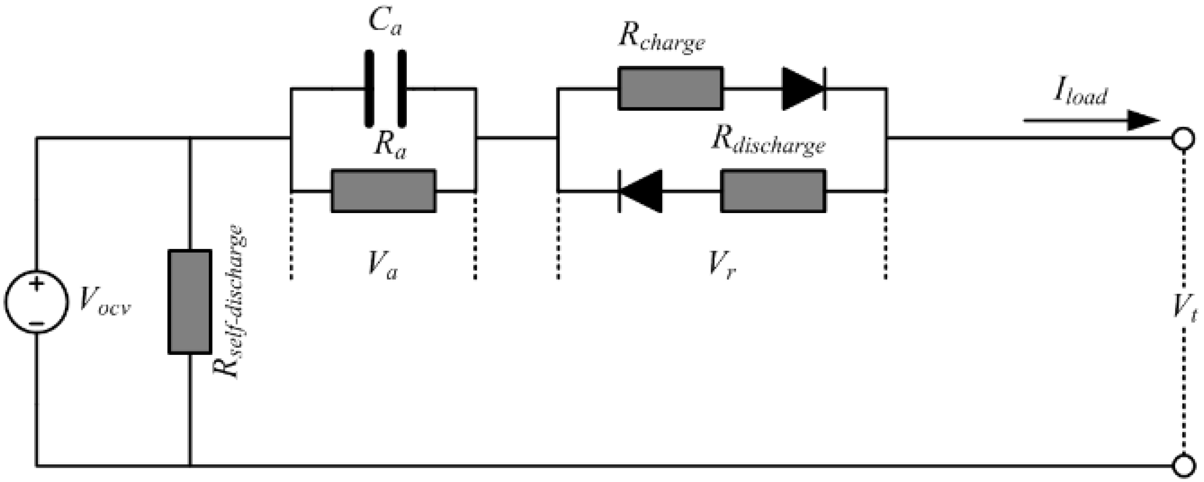
2.1. Modelling of Battery

To examine the state and dynamic behavior of a lithium-ion battery, an accurate and reliable battery model must be developed first. Several types of ECMs for the modelling of lithium-ion batteries have been reported [48]. Generally, the accuracy and battery dynamics are enhanced by increasing the order of ECM. In this case, however, the computing complexity of the system increases. Therefore, the first order resistor and capacitor (RC) network, as shown in Figure 1, was adopted to cope with the trade-off between the modelling accuracy and complexity. The battery model can be divided easily into four main parts. In the first part voltage source represents the open circuit voltage (V_ocv). In the second part, a self-discharge resistor (R_{self-discharge}) is used to describe the self-energy loss when the battery charge is stored for a long time. In a lithium-ion battery, the self-discharge can be ignored because self-discharge in a lithium-ion battery is 2%–10% per month, so R_{self-discharge} can be set to infinity [49]. The inner ohmic resistance of a battery (R_i) (R_charge at charge and R_discharge at discharge condition) is in the third part. In the last part, in the parallel RC network electrochemical diffusion resistance (R_a) and electrochemical diffusion capacitance (C_a) are used to model the transient dynamic behavior of a battery during the charging and discharging condition. The values of these battery parameters are highly depending upon the SOC and operating temperature of the battery. So, the accuracy of these battery parameters is so much important to measure SOC accurately.

Where $I_{load}$ is the load current. The electrical behavior of a used battery model can be expressed using the following equations:

$$\dot{V_a}=-\frac{1}{C_a{R}_a}{V}_a+\frac{1}{C_a}{I}_{load}$$

(1)

and:

$$V_t=V_{ocv}-V_a-V_r$$

(2)

where $V_a$ is the voltage across $C_a$ and $R_a$, and $V_r$ is the voltage across resistor $R_i$. Therefore:

$$V_r=\{\begin{array}{l}{I}_{load}\times R_{discharge} \left(discharge\right)\\ \begin{array}{l}-I_{load}\times R_{charge}\hspace{1em}\left(charge\right)\\ I_{load}{R}_i\end{array}\end{array}$$

(3)

The Samsung ICR18650-26F lithium cobalt oxide (LICoO₂) battery was used to perform the SOC-OCV; it has a rated capacity of 2600 mAh. The test was performed under a controlled temperature of 27 ± 1 °C. Initially, the battery was fully charged using the conventional technique (constant current constant voltage) until it reached the charge termination voltage (4.05 V [50]). When the battery was fully charged, the SOC of the battery was considered to be 100%. After pausing of 1 hour for depolarization, the battery was discharged using pulses of 1000 mA for an interval of 430 s until it reached the discharge cut-off voltage (2.75 V [50]). At the end of complete discharge, the SOC of the battery was considered to be 0%. The cell was left in the open circuit after each discharge pulse for a period of one hour to measure the discharge OCVs [51]. A similar process was performed to measure the charge OCVs of a battery from 0% to 100% SOC during charging. After the pulse charging and discharging test, the average charge and discharge OCVs were treated as the real OCVs. As the OCV and SOC is intrinsically nonlinear, the function of $V_{ocv}$ in terms of SOC can be expressed as:

$$V_{ocv}=f\left(z\right)=p_1{z}^7+p_2{z}^6+p_3{z}^5+p_4{z}^4+p_5{z}^3+p_6{z}^2+p_{7}z+p_8$$

(4)

where $z$ is the value of SOC of a battery. $p_1$, p₂, $p_3$, $p_4$, $p_5$, $p_6$, $p_7$, and $p_8$ are the extracted polynomial coefficients using the curve-fitting toolbox in MATLAB^TM; it fits the OCV values precisely under different SOC values, as shown in Figure 2. These equations can be used to formulate a complete state-space approach for the development of a BMS.

Table 1. Values of the polynomial Coefficients of the SOC-OCV function.

Polynomial Coefficients	Polynomial Coefficients Values
$p_1$	$4.649\times {10}^{-13}$
$p_2$	$-1.592\times {10}^{-10}$
$p_3$	$2.125\times {10}^{-08}$
$p_4$	$-1.402\times {10}^{-06}$
$p_5$	$4.938\times {10}^{-05}$
$p_6$	$-0.001067$
$p_7$	$0.02336$
$p_8$	$3.221$

lists the values of these coefficients.

2.2. Lagrange Multiplier Method for Online Model Identification

The discrete form of Equations (1) and (2) can be derived by using the zero order hold method [52] i.e., $H\left(z\right)=\left(1-z^{-1}\right)𝒵\left({ℒ}^{-1}\left\{\frac{H\left(s\right)}{s}\right\}\right)$. By applying Laplace transform to Equation (1), we get:

$$s{V}_a\left(s\right)-V_a\left(0\right)=-\frac{1}{C_a{R}_a}{V}_a\left(s\right)+\frac{1}{C_a}{I}_{load}\left(s\right)$$

(5)

By substituting $V_a\left(0\right)$ = 0 and rearranging Equation (5), it can be written as:

$$H\left(s\right)=\frac{V_a\left(s\right)}{I_{load}\left(s\right)}=\frac{1}{C_a\left(s+\frac{1}{C_a{R}_a}\right)}$$

(6)

By applying zero order hold method, Equation (6) can be reduced to:

$$H\left(z\right)=\frac{R_a\left(1-e^{-\frac{\Delta t_d}{C_a{R}_a}}\right)z^{-1}}{\left(1-z^{-1}{e}^{-\frac{\Delta t_d}{C_a{R}_a}}\right)}$$

(7)

By applying inverse $z$-transform, the discrete form of the above equation is the following:

$$V_a^{k+1}=V_a^k\mathit{exp}\left(\frac{-\Delta t_d}{R_a{C}_a}\right)+I_{load}^k{R}_a\left[1-\mathit{exp}\left(\frac{-\Delta t_d}{R_a{C}_a}\right)\right]$$

(8)

Similarly, Equation (2) can be rewritten in time discrete form as:

$$V_t^k=V_{ocv}^k-V_a^k-I_{load}^k{R}_i$$

(9)

where $\Delta t_d$ is the sampling interval; $k$ is discrete time index and it is a non-negative integer number because estimation starts at $t=0$ second. $V_t^k, V_{ocv}^k,$ and $V_a^k$ are the terminal, open circuit and diffusion voltages, respectively, at the $k$th sampling time, and the load current at the $k$th sampling time is $I_{load}^k$. Using Equation (8), Equation (9) becomes:

$$V_t^{k+1}=V_{ocv}^{k+1}-\left[V_a^k\mathit{exp}\left(\frac{-\Delta t_d}{R_a{C}_a}\right)+I_{load}^k{R}_a\left\{1-\mathit{exp}\left(\frac{-\Delta t_d}{R_a{C}_a}\right)\right\}\right]-I_{load}^{k+1}{R}_i$$

(10)

$E_t^k$ is defined as Equation (11):

$$E_t^k=V_t^k-V_{ocv}^k$$

(11)

Therefore, Equation (10) can be rewritten as:

$$E_t^{k+1}=-\left[V_a^k\mathit{exp}\left(\frac{-\Delta t_d}{R_a{C}_a}\right)+I_{load}^k{R}_a\left\{1-\mathit{exp}\left(\frac{-\Delta t_d}{R_a{C}_a}\right)\right\}\right]-I_{load}^{k+1}{R}_i$$

(12)

By putting the value of $V_a^k=-E_t^k-I_{load}^k{R}_i$ in the above Equation, it becomes:

$$E_t^{k+1}=E_t^k\mathit{exp}\left(\frac{-\Delta t_d}{R_a{C}_a}\right)+I_{load}^k{R}_i\mathit{exp}\left(\frac{-\Delta t_d}{R_a{C}_a}\right)-I_{load}^k{R}_a\left[1-\mathit{exp}\left(\frac{-\Delta t_d}{R_a{C}_a}\right)\right]-I_{load}^{k+1}{R}_i$$

(13)

By rearranging Equation (13), it becomes:

$$E_t^{k+1}=E_t^k\mathit{exp}\left(\frac{-\Delta t_d}{R_a{C}_a}\right)+\left(-R_i\right)I_{load}^{k+1}+\left(R_i\mathit{exp}\left(\frac{-\Delta t_d}{R_a{C}_a}\right)-R_a\left\{1-\mathit{exp}\left(\frac{-\Delta t_d}{R_a{C}_a}\right)\right\}\right)I_{load}^k$$

(14)

Therefore, the above Equation (14) can be rewritten as:

$$E_t^{k+1}={\beta }_1{E}_t^k+{\beta }_2{I}_{load}^k+{\beta }_3{I}_{load}^{k+1}$$

(15)

where:

$$\begin{array}{l}{\beta }_1=\mathit{exp}\left(\frac{-\Delta t_d}{R_a{C}_a}\right)\hfill \\ {\beta }_2=R_i\mathit{exp}\left(\frac{-\Delta t_d}{R_a{C}_a}\right)-R_a\left\{1-\mathit{exp}\left(\frac{-\Delta t_d}{R_a{C}_a}\right)\right\}\hfill \\ {\beta }_3=-R_i\hfill \end{array}\}$$

(16)

and:

$$\begin{array}{l}{R}_i=-{\beta }_3\hfill \\ R_a=\frac{{\beta }_1{\beta }_3+{\beta }_2}{{\beta }_1-1}\hfill \\ C_a=\frac{\left(1-{\beta }_1\right)\Delta t_d}{({\beta }_1{\beta }_3+{\beta }_2)\log \left({\beta }_1\right)}\hfill \end{array}\}$$

(17)

Defining:

$$\begin{array}{c}{E}_t^{k+i}=y \left(k+i\right);\hspace{1em}\hspace{1em}\hspace{1em}\hspace{1em}for i=1, 2, 3, \dots , N\\ E_t^{k+i}=x_1 \left(k+i+1\right);\hspace{1em}\hspace{1em}for i=0, 1, 2, \dots , N\\ I_t^{k+i}=x_2 \left(k+i\right);\hspace{1em}\hspace{1em}\hspace{1em}\hspace{1em}for i=1, 2, 3, \dots , N\\ I_t^{k+i}=x_3 \left(k+i+1\right);\hspace{1em}\hspace{1em}for i=0, 1, 2, \dots , N\\ \mathit{x}\left(k\right)=\left[\begin{array}{ccc}{E}_t^k& I_{load}^k& I_{load}^{k+1}\end{array}\right]\end{array}\}$$

(18)

Suppose:

$$\left[\begin{array}{c}y\left(k+1\right)\\ \begin{array}{c}y\left(k+2\right)\\ \begin{array}{c}⋮\\ y\left(k+N\right)\end{array}\end{array}\end{array}\right]=\left[\begin{array}{c}\begin{array}{cc}{x}_1\left(k+1\right)& \begin{array}{cc}{x}_2\left(k+1\right)& x_3\left(k+1\right)\end{array}\end{array}\\ \begin{array}{c}\begin{array}{cc}{x}_1\left(k+2\right)& \begin{array}{cc}{x}_2\left(k+2\right)& x_3\left(k+2\right)\end{array}\end{array}\\ \begin{array}{c}\begin{array}{ccc}⋮& \hspace{1em}\hspace{1em}⋮& \hspace{1em}\hspace{1em}⋮\end{array}\\ \begin{array}{cc}{x}_1\left(k+N\right)& \begin{array}{cc}{x}_2\left(k+N\right)& x_3\left(k+N\right)\end{array}\end{array}\end{array}\end{array}\end{array}\right]\left[\begin{array}{c}{\beta }_1\\ \begin{array}{c}{\beta }_2\\ {\beta }_3\end{array}\end{array}\right]$$

(19)

or:

$$y\left(k\right)=\mathit{x}\left(k\right)\mathit{\beta }\left(k\right)$$

(20)

$$\mathit{\beta }={\left[\begin{array}{ccc}{\beta }_1& {\beta }_2& {\beta }_3\end{array}\right]}^T$$

(21)

Suppose $\widehat{\mathit{\beta }}\left(k\right)$ and $\widehat{\mathit{\beta }}\left(k-1\right)$ are the adjacent weight vectors of the model describer in Equation (19). The objective is to find a weight vector $\mathit{\beta }$ with stable values that satisfy all the data, i.e., $\forall k=1, 2, 3, \dots , N.$ Thus, to achieve this, the target is to minimize the difference in the two consecutive weight vector steps as follows:

$$\delta \widehat{\mathit{\beta }}\left(k\right)=\widehat{\mathit{\beta }}\left(k\right)-\widehat{\mathit{\beta }}\left(k-1\right)$$

(22)

Subject to N constraints:

$$y\left(k+n\right)={\mathit{x}}^T\left(k+n\right)\widehat{\mathit{\beta }}\left(k+n\right)+ϵ\left(k+n\right);\hspace{1em}n=1,2,3,\dots ,N.$$

(23)

$ϵ$ is the difference of the model output and actual data at the kth sample time. Define a cost function using the Lagrange multiplier method to formulate the above problem into an optimization environment:

$$J\left(k\right)=\Vert \widehat{\mathit{\beta }}\left(k\right)-\widehat{\mathit{\beta }}{\left(k-1\right)\Vert }^2+{\displaystyle \sum }_{n=1}^N{\lambda }_k\left(\begin{array}{c}y\left(k+n\right)-{\mathit{x}}^T\left(k+n\right)\widehat{\mathit{\beta }}\left(k+n\right)\\ -ϵ\left(k+n\right)\end{array}\right)$$

(24)

where ${\lambda }_k$’s are the Lagrange multipliers and can be determined as follows:

$$\mathit{\lambda }={\left[{\lambda }_1, {\lambda }_2, {\lambda }_3, \dots ,{\lambda }_N\right]}^T$$

(25)

Using Equations (20), (23) and (25), Equation (24) can be rewritten as:

$$J\left(k\right)=\Vert \widehat{\mathit{\beta }}\left(k\right)-\widehat{\mathit{\beta }}{\left(k-1\right)\Vert }^2+{\left(\mathit{y}\left(k\right)-\mathrm{X}\left(k\right)\widehat{\mathit{\beta }}\left(k+n\right)-ϵ\left(k\right)\right)}^T\mathit{\lambda }$$

(26)

The extreme values of the above cost function can be found by differentiating it with respect to the weight vector and setting the first derivative equal to zero, i.e.:

$$\delta \widehat{\mathit{\beta }}\left(k\right)=\frac{1}{2}{\mathrm{X}}^T\left(k\right)\mathit{\lambda }$$

(27)

Using Equations (19) and (22), and Lagrange multiplier method we can find:

$$\mathit{\lambda }=2{\left(\mathrm{X}\left(k\right){\mathrm{X}}^T\left(k\right)\right)}^{-1}\mathit{e}\left(k\right)$$

(28)

and:

$$\mathit{e}\left(k\right)=\mathit{y}\left(k\right)-\mathrm{X}\left(k\right)\widehat{\mathit{\beta }}\left(k-1\right)$$

(29)

Substituting this value of the Lagrange multiplier vector into Equation (27) results in:

$$\delta \widehat{\mathit{\beta }}\left(k+1\right)={\mathrm{X}}^T\left(k\right){\left(\mathrm{X}\left(k\right){\mathrm{X}}^T\left(k\right)\right)}^{-1}\mathit{e}\left(k\right)$$

(30)

To apply the above-derived Equation in an adaptive algorithm, a controlling parameter could be added as follows. This parameter is used for convergence:

$$\delta \widehat{\mathit{\beta }}\left(k+1\right)=\mu {\mathrm{X}}^T\left(k\right){\left(\mathrm{X}\left(k\right){\mathrm{X}}^T\left(k\right)\right)}^{-1}\mathit{e}\left(k\right)$$

(31)

Equation (31) can be rewritten using Equation (22):

$$\widehat{\mathit{\beta }}\left(k+1\right)=\widehat{\mathit{\beta }}\left(k\right)+\mu {\mathrm{X}}^T\left(k\right){\left(\mathrm{X}\left(k\right){\mathrm{X}}^T\left(k\right)\right)}^{-1}\mathit{e}\left(k\right)$$

(32)

In some of cases, during application of this algorithm, numerical difficulties have been reported [53]. Therefore, to avoid such numerical difficulties, a parameter $\delta$ could be added (if required):

$$\widehat{\mathit{\beta }}\left(k+1\right)=\widehat{\mathit{\beta }}\left(k\right)+\mu {\mathrm{X}}^T\left(k\right){\left(\mathrm{X}\left(k\right){\mathrm{X}}^T\left(k\right)+\delta \mathrm{I}\right)}^{-1}\mathit{e}\left(k\right)$$

(33)

Figure 3 presents a flow chart of the proposed technique.

3. Adaptive SOC Estimator Design

Based on the data-driven identified parameters of battery model, an online estimation of SOC is designed in this section. The SOC of the battery can be inferred precisely using the inverse of Equation (4) if the OCV of the battery is known. The design of the OCV estimator discussed below.

3.1. Adaptive OCV Estimator Design

Using Equation (16), the discrete form of Equations (1) and (2) can be written as:

$$V_a^k=V_a^{k-1}{\beta }_1+I_{load}^{k-1}{R}_a\left[1-{\beta }_1\right]$$

(34)

$$V_a^{k-1}=V_{ocv}^{k-1}-V_t^{k-1}-I_{load}^{k-1}{R}_i$$

(35)

Placing Equation (35) into Equation (34) yields:

$$V_{ocv}^k=V_{ocv}^{k-1}{\beta }_1-[V_t^{k-1}+I_{load}^{k-1} R_i]{\beta }_1+I_{load}^{k-1} R_a\left[1-{\beta }_1\right]+V_t^k+I_{load}^k R_i$$

(36)

By assuming that the OCV is a slow varying function, then $V_{ocv}^k=V_{ocv}^{k-1}$, so the OCV can be solved as follows:

$$\widehat{V_{ocv}^k}=\frac{V_t^k+I_{load}^k{R}_i-[V_t^{k-1}+I_{load}^{k-1}{R}_i]{\beta }_1+I_{load}^{k-1}{R}_a\left[1-{\beta }_1\right]}{1-{\beta }_1}$$

(37)

A smaller sampling time has the advantage of producing an estimated model with better accuracy.

3.2. Adaptive SOC Estimator Design

The SOC of a battery can be defined as the percentage of currently available capacity with respect to the current maximum available battery capacity [8,9,10,11]. The SOC in terms of the time function can be written as:

$$z\left(t\right)=z\left(t_o\right)-\frac{1}{Q_m}{{\displaystyle \int }}_{t_o}^t\eta i\left(t\right)dt$$

(38)

where $z\left(t\right)$ is the SOC of a battery at the sampling time $t$, $z\left(t_o\right)$ is the initial SOC value, $i\left(t\right)$ is the instantaneous load current (considered positive for the discharging and negative for charging phase), and $Q_m$ is the present maximum available battery capacity. This differs from the rated capacity due to the aging effect of the battery. $\eta$ is the Columbic efficiency of a battery. The Columbic efficiency depends mainly on the temperature, capacity, and battery current. In this paper, $\eta$ = 1. Equation (38) can be written in discrete form as follows:

$$z^k=z^{k-1}-\frac{\eta i^k\Delta t_d}{Q_m}$$

(39)

From Equation (4), it is evident that the VOC is a function of the SOC, so it can be rewritten as:

$$\begin{array}{c}z=f^{-1}\left(V_{ocv}\right)\\ \widehat{z}=f^{-1}\left(\widehat{V_{ocv}}\right)\end{array}\}$$

(40)

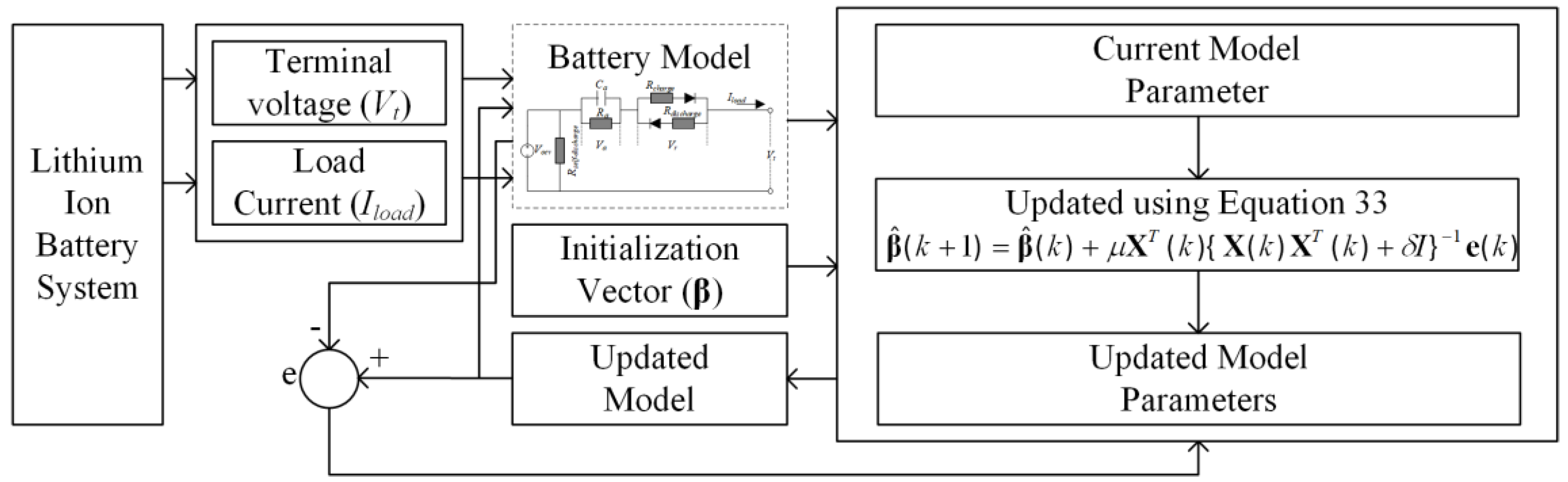
3.3. Algorithm Estimation Approach

From the above descriptions, the OCV of a battery has a direct relationship with the battery SOC estimation. An accurate and precise SOC estimation requires a reliable OCV estimator. In this paper, a Lagrange multiplier method was proposed to identify the data driven parameters. The proposed method provides accurate real-time parameters for a reliable SOC estimation. Figure 4 shows a general diagram of the proposed methodology.

Step 1: Data measurements. The real time battery current and voltage are monitored and measured during the battery charging and discharging time. The data is saved for each sample interval. In this work, MATLAB^TM was used to run the proposed algorithm. Although the battery data (voltage and current) are in non-real-time, it is a time series computation process; hence, the proposed methodology is appropriate for real time applications.

Step 2: Battery parameter identification. The voltage and current are measured during battery charging and discharging. The Lagrange multiplier method is used to calculate the data-driven battery parameters, as discussed in Section 2. The Lagrange method continuously trying to reduce the error to reach the optimal values of parameters.

Step 3: Adaptive SOC estimation. First, the data driven parameters are used to estimate the OCV of a battery using Equation (37). The estimated OCV is used to estimate the SOC of the battery using Equation (40).

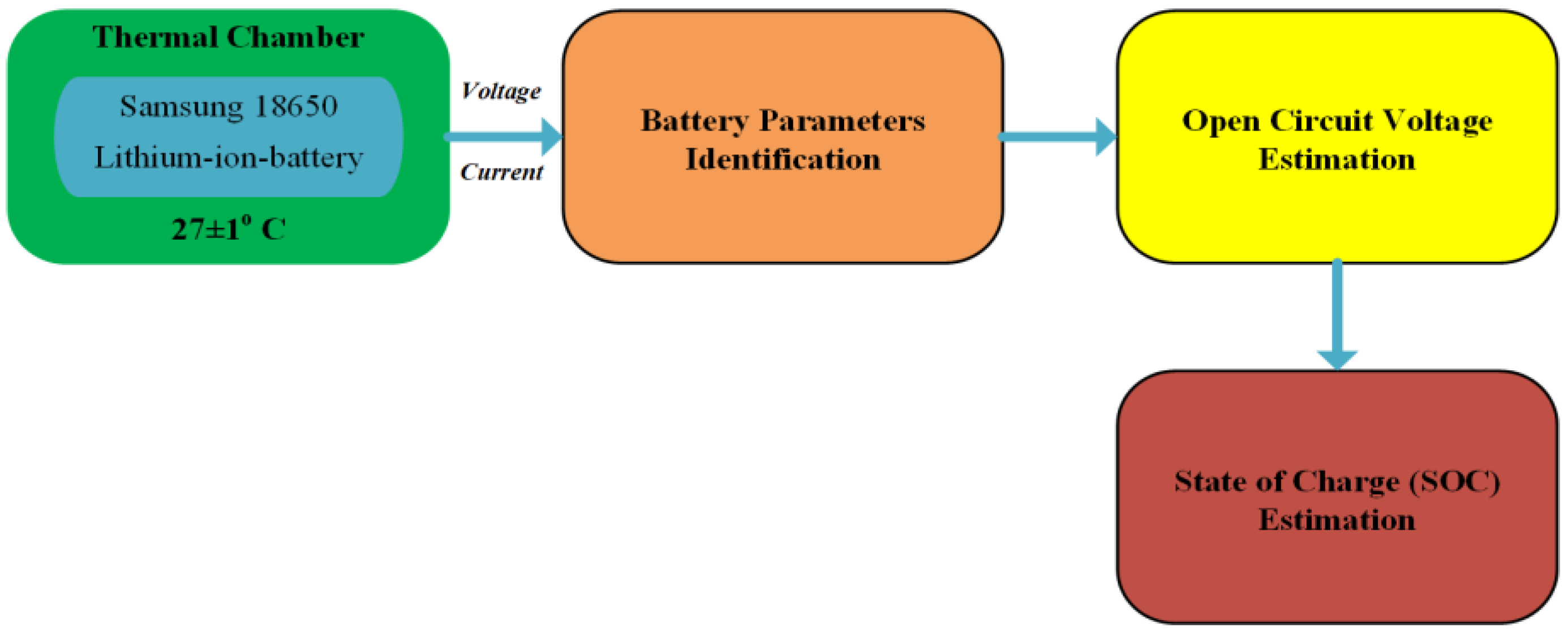
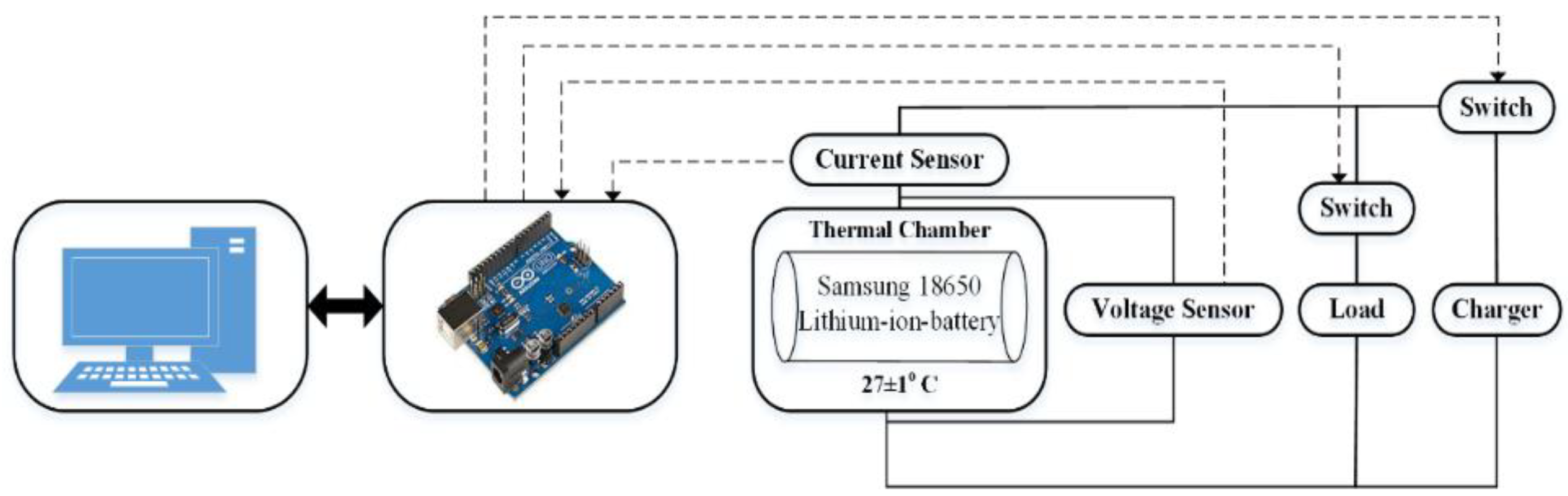
4. Experimental Setup

Figure 5 shows the experimental configuration of the test system. The Samsung 18650 lithium-ion-battery (2600 mAh) was used in the experiments. The battery was positioned inside a thermal chamber to maintain a battery temperature of 27 ± 1 °C. The voltage and current sensors were used to measure the voltage and charge/discharge current at 1 second sample rate. The sensors had a maximum inaccuracy of 0.5%. The Arduino Uno interfaced with MATLAB^TM Simulink was used to control the charge/discharge cycle and store sensor data in a computer. The battery was charged using a Naydrone Volter battery charger (Drong Zhang Co Ltd, Seoul, South Korea). The battery was discharged at different constant currents to check the validity of the proposed methodology. The actual SOC of the battery was measured using the ampere hour counting method. Other details of the experiment were discussed at the end of Section 2.1.

5. Results and Discussion

Rechargeable batteries play a pivotal role in renewable energy storage, EVs production, and portable electronic appliances. The BMS system of the battery must be well designed. The SOC of the battery is one of the major indicators in the BMS. The SOC can be perceived as the fuel gauge of the battery. Therefore, an estimation of the SOC is a crucial part of the BMS.

Figure 1 shows a schematic diagram of the battery model. The first order RC battery model was selected considering the tradeoff between the complexity and accuracy. Figure 2 presents the relationship between the OCV and SOC of the battery. The relationship between the OCV and SOC was developed using the curve-fitting toolbox in MATLAB^TM. Table 1 lists the polynomial coefficients. Figure 3 shows the flow chart to identify the data-driven parameters of the battery using the proposed technique. Figure 4 shows the general layout of the proposed methodology to estimate the OCV and SOC of the battery. Figure 5 presents the experimental setup of the proposed work. Figure 6a–c shows the online identified parameters of a lithium-ion-battery and their respective errors with the reference values. Figure 7 shows the estimated SOC of a battery using the proposed method and its comparison with the reference and fixed parameter SOC estimation. This also shows the error during the estimation of the SOC. Figure 8 shows the robustness and accuracy of proposed algorithm in hybrid pulse experiment. Figure 9 compares the reference and estimated SOC with different initial SOCs. Figure 10 presents the estimated remaining capacity of the battery.

Table 2. CPU time comparison of the proposed and other methodologies.

	Proposed Method	RLS [56]	VRLS-KF [55]	Non-Updating EKF [55]	RLS-EKF [55]
Computational time (µs)	63.472	59.379	66.525	75.762	107.385

and

Table 3. Performance comparison of the proposed and other methodologies.

	Proposed Method	RLS [56]	FBCRLS Based Observer [54]	RLS-EKF [54]
Convergence time (s)	81	305	167	268
MAE	0.94%	1.93%	0.81%	1.65%

summarize the performance of the proposed algorithm. Figure 11a–c shows the sensitivity analysis under different sampling time and sensors error.

The proposed Lagrange multiplier methodology was implemented on the experimental data acquired in discharge test using MATLAB^TM. To check the validity of the proposed methodology, the algorithm was initialized with a random value of battery parameters. In this study, the initializing battery parameters values were $R_i$ = 3 mΩ, $R_a$ = 35 mΩ, and $C_a$ = 2500 F.

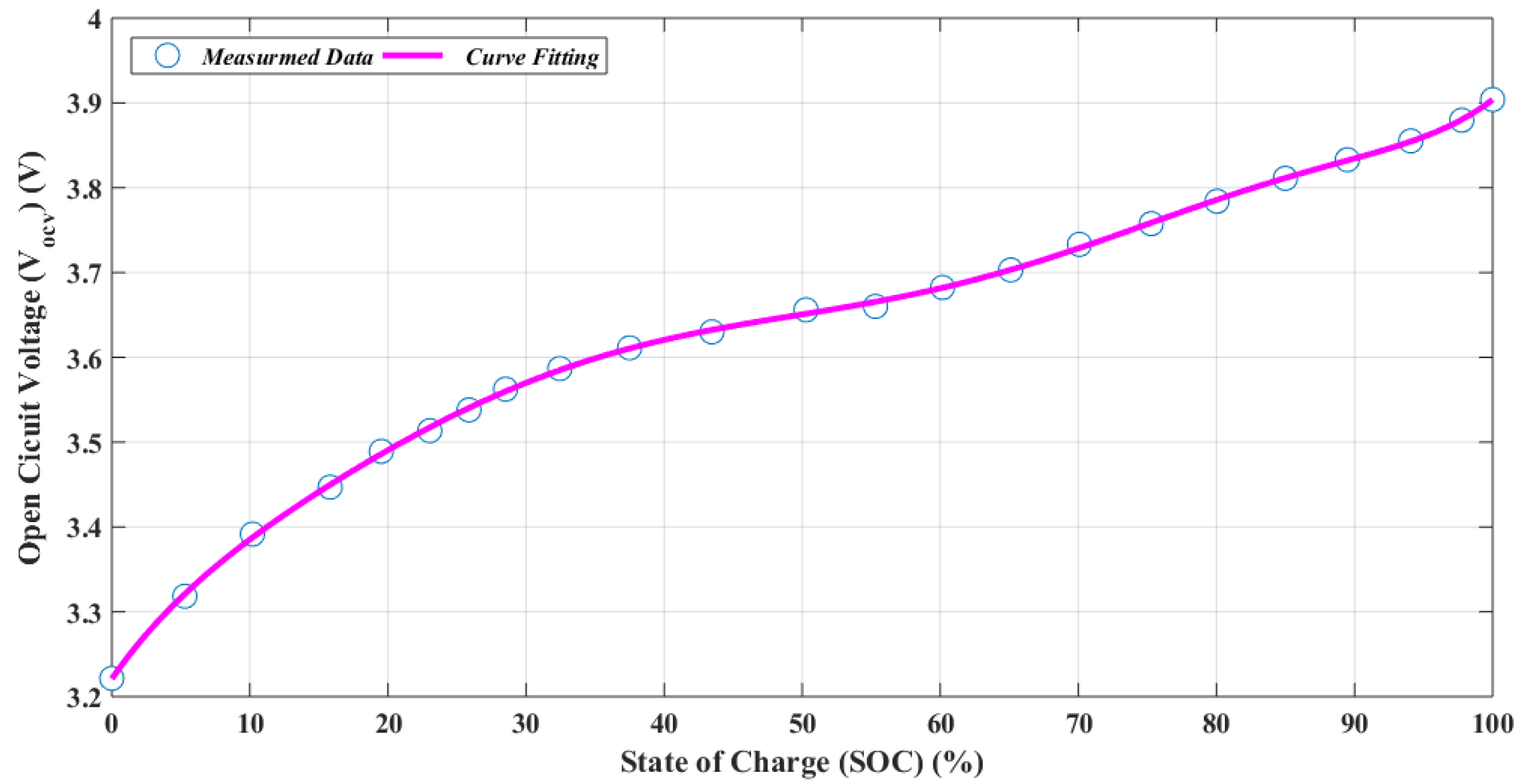
5.1. Battery Parameters Identification

The accuracy of the battery parameters is essential for estimating the SOC. To evaluate the accuracy of model identification, the reference value of the battery parameters should be known. The reference values of the battery parameters can be determined at the average points of the charge and discharge pulse test. These reference values were extracted offline, and the final reference value of each parameter was determined by taking the average of all points. The reference inner ohmic resistance of the battery, $R_i$, can be extracted by calculating the change in voltage and step change in current at each time point, i.e., $R_i=\left(V_{ocv}-V_t\right)/\Delta I_{load}$. Because $V_{ocv}$ and $V_r$ are calculated, the value of $V_a$ can be determined using Equation (2). The $R_a$ and $C_a$ can be extracted using the following equation [54]:

$$V_a^k=\left[V_a^{k-1}{I}_{load}^{k-1}\right]\left[\begin{array}{c}\mathit{exp}\left(\frac{-\Delta t_d}{R_a{C}_a}\right)\\ 1-\mathit{exp}\left(\frac{-\Delta t_d}{R_a{C}_a}\right)R_a\end{array}\right]$$

(41)

Figure 6a–c show the data driven identified parameters ($R_i$, $R_a$, and $C_a$) and their respective error with fixed values, respectively. All the parameters are time varying and dependent on the SOC, because fixed parameters are flawed in that they cannot adjust their values according to the working conditions and battery aging. The convergence rate of the proposed methodology was very high despite the erroneous initialization. This tracks the change in the model parameters accurately throughout the working cycle. The error was high at the start-up stage because the proposed methodology requires some time to converge from the initialization error.

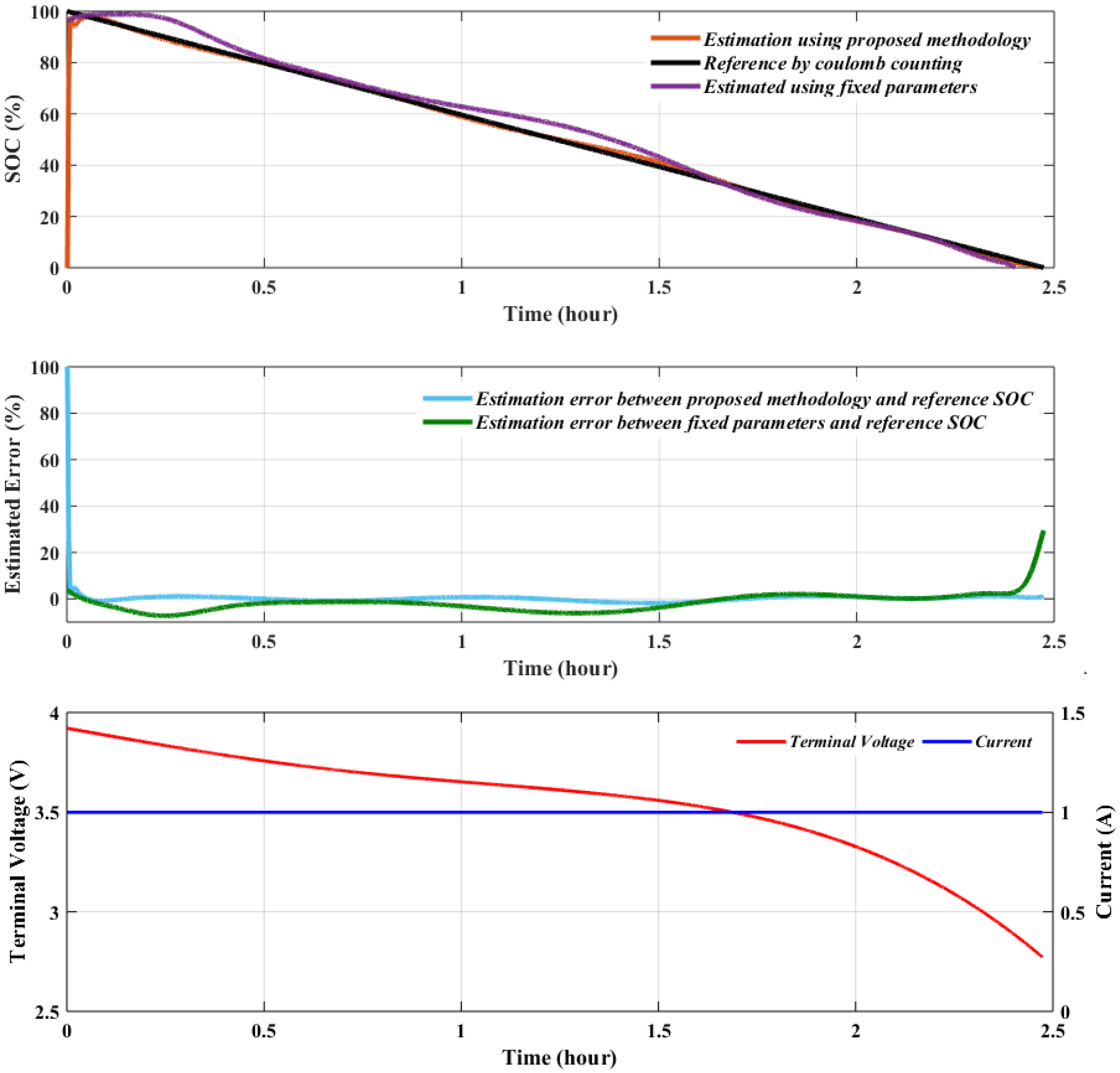
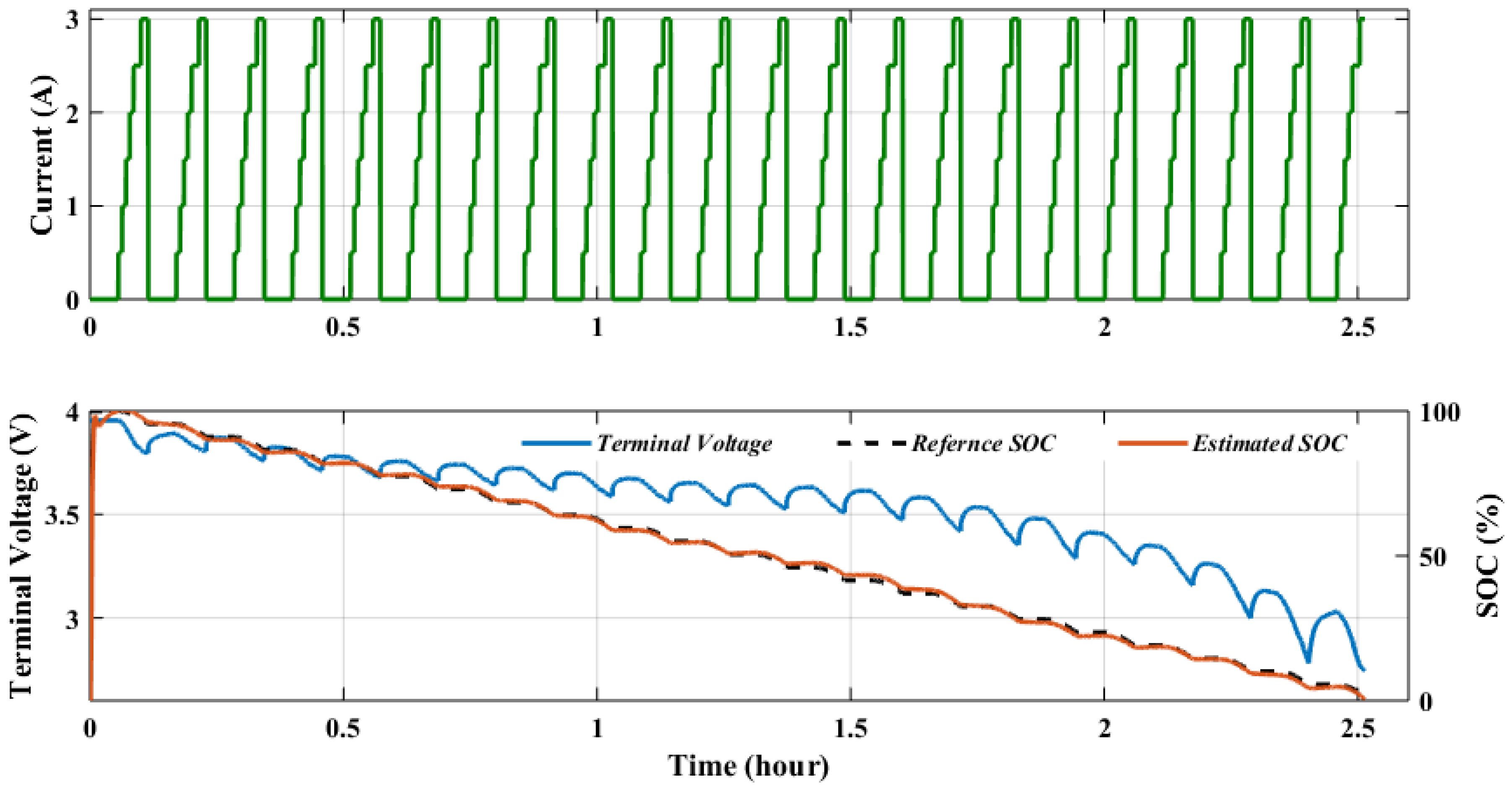
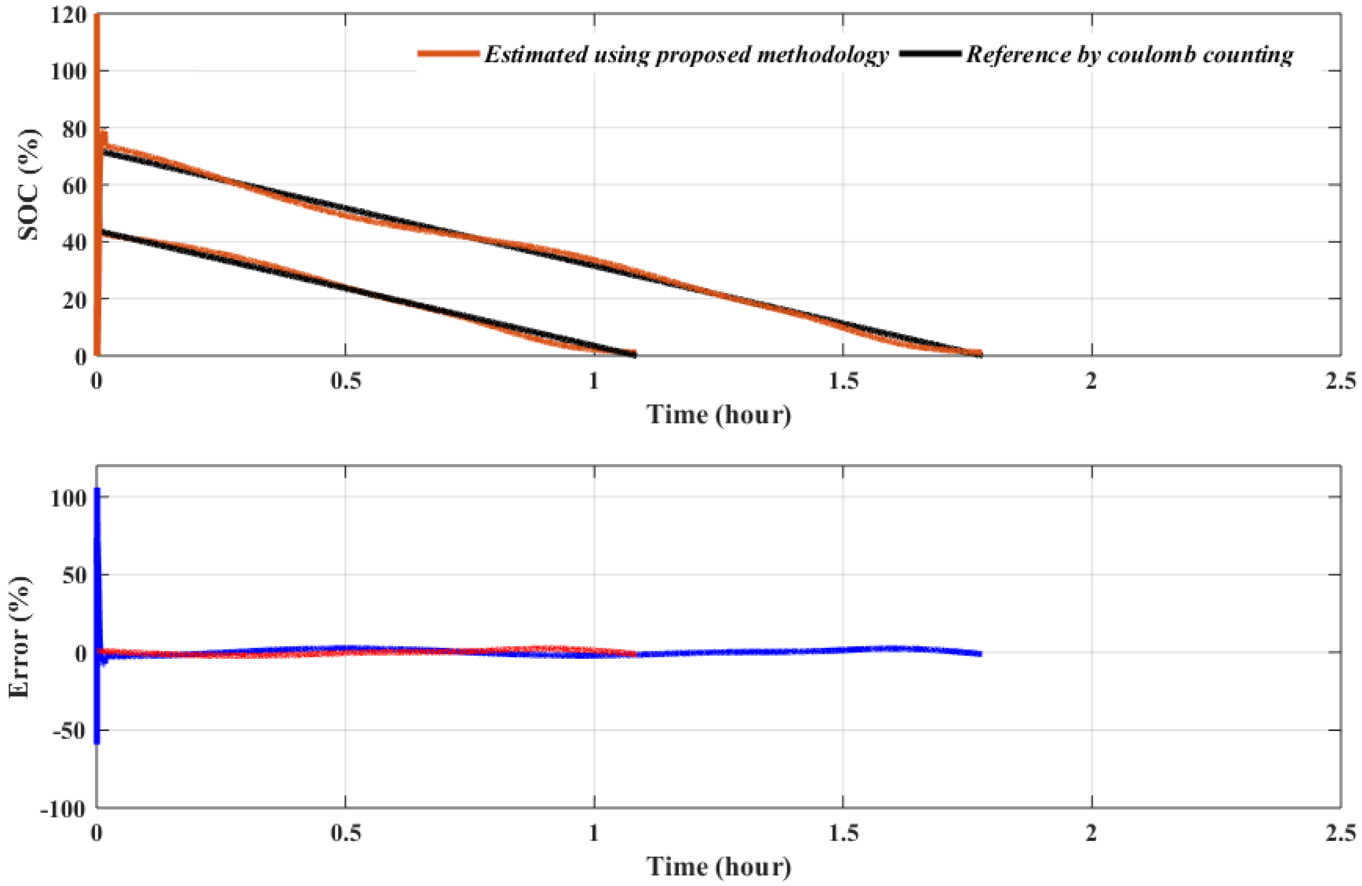
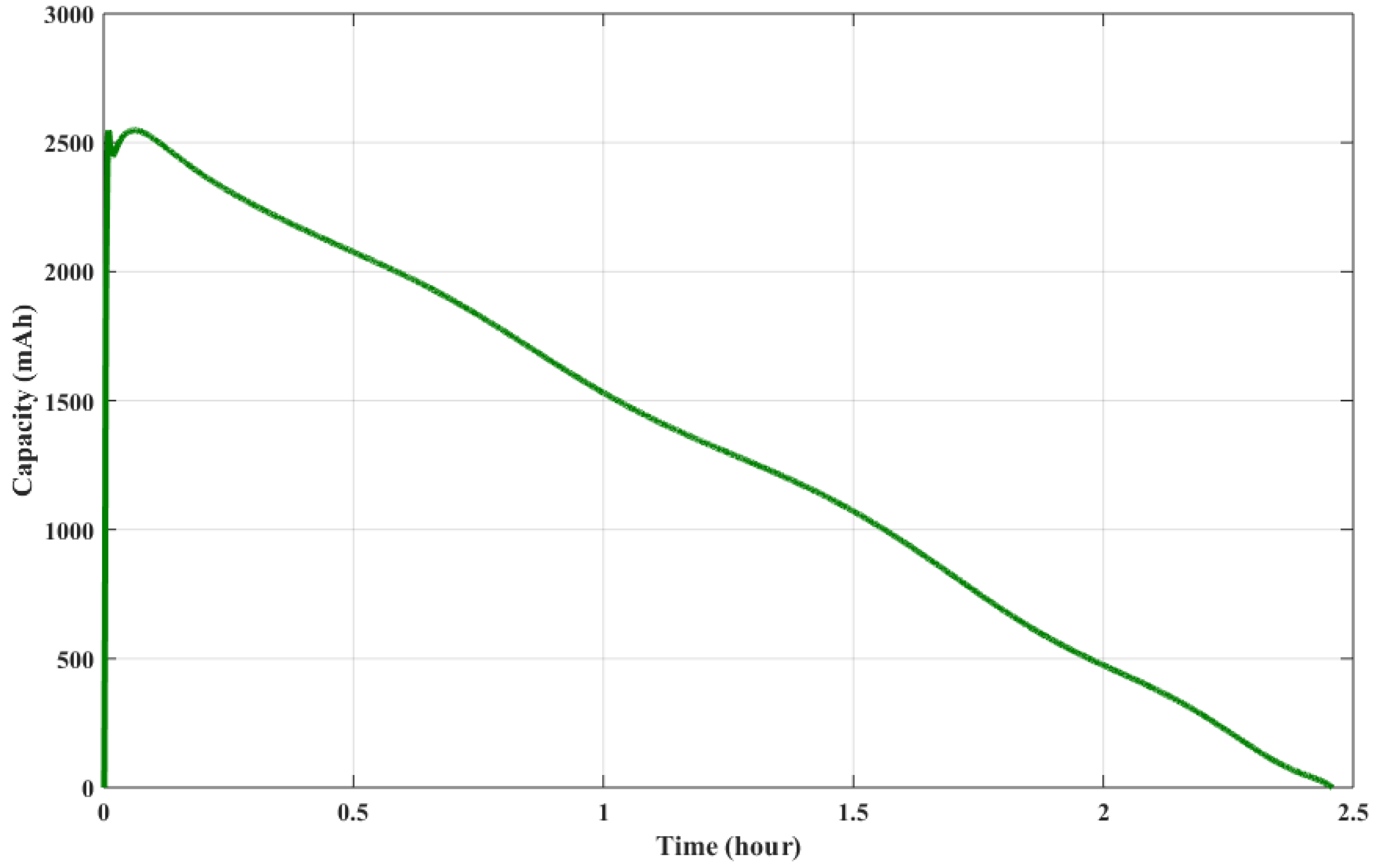
5.2. Performance of SOC Estimator of Battery

After determining the data-driven parameters of the battery, the OCV and SOC can be estimated at each sampling interval. Figure 7 shows the SOC and error profiles of the proposed methodology, fixed parameters estimation, and reference trajectory. It also shows the discharge current and terminal voltage profiles. The reference trajectory of the lithium-ion-battery was measured using the ampere-hour counting method. The initial SOC value was set to 100%. The proposed methodology tracked the reference SOC robustly, stably and accurately after an initial error correction. The proposed algorithm had a maximum error of 1.28% and the fixed parameters had a 7.28% maximum error during the entire estimation. The high error of the proposed method was between 45% to 35% SOC because at the particle point, the SOC-OCV curve shown in Figure 2 has a very small slope. The small slope causes some error in estimating the SOC in Equation (40). The presence of this error was also discussed by Wei et al. [54].

Figure 8 shows the results of the proposed approach for hybrid pulse experiment test. The proposed algorithm shows same robustness and accuracy in the presence of different discharging pulses. The terminal voltage, pulse discharge current, estimated SOC and reference SOC profiles has shown in Figure 8.

Figure 9 presents the estimated SOC with different initial SOCs and their respective errors. The proposed methodology showed a good convergence rate at different initial SOC. Figure 10 shows the estimated remaining capacity of the battery during discharge.

5.3. Computational Time

The computational complexity of the proposed methodology was compared with other existing methods reported in the literature [55]. A gradient approach-based optimization of a given problem has been used frequently in the past. Such algorithms have a favorable position because of their less computational efforts and efficient convergence in constrained and unconstrained environments. In particular, for a constraint environment, it would be beneficial is all the constraints and objective function could be combined in a single cost function that is extremized. The Lagrange multiplier method provides this feature to convert the given constraints to a function with a zero value and add them individually in the objective function. These added constraints have no effect in the function value of the objective function but at the same time, the objective function inherits the constraints defined in a particular problem. Therefore, the combination of the gradient approach and Lagrange multiplier method not only makes the problem simpler, but also solves it with less computational load and efficient convergence. To determine the computational complexity of the proposed methodology, the algorithm was run 10 times. The proposed algorithm was run on a desktop-PC, with the following specifications: 3.4 GHz CPU and 8.0 GB RAM. Table 2 compares the CPU time comparison of the methodologies.

The proposed estimator used 40.89% less time than the RLS-EKF. The KF approaches were too complex as compare with the proposed methodology, which is why the computational time of the KF are high.

5.4. Convergence Rate

The evaluate the performance of the proposed algorithm, the mean absolute error (MAE) was used to compare the accuracy of the proposed algorithms with other algorithms published in the literature [54,55,56]. The convergence time is defined as an estimation error within 5% [54]. This is used to evaluate the convergence characteristics of the algorithms. Table 3 compares the proposed and other methodologies.

The convergence speed of the proposed methodology was remarkably low in the presence of erroneous initialization. The convergence time can be decreased further using the SOC close to a real value, and estimated using the OCV before start of the algorithm. In this study, the initial SOC was set to 0% to check the convergence speed of the proposed methodology.

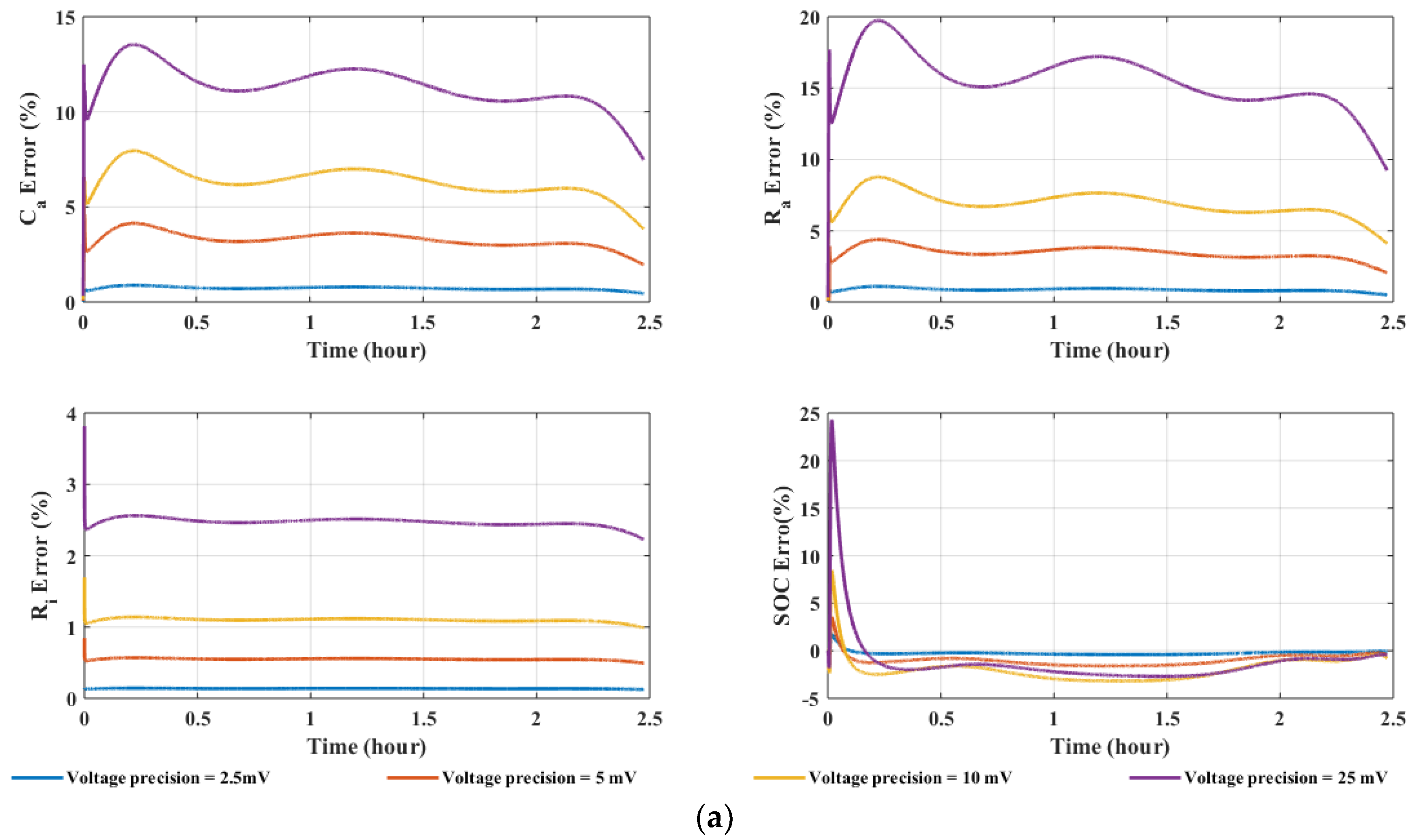
5.5. Sensitivity Analysis

In this section, the accuracy of the parameter identification and SOC estimation has been evaluated using simulations under following scenarios: (i) voltage sensor accuracy (±2.5, ±5, ±10, and ±25 mV), (ii) current sensor accuracy (±5, ±50, ±100, and ±500 mA) and (iii) sampling time (0.1, 0.4, 0.7, and 0.95 s). The estimated parameters were compared with reference values to determine the effect on the accuracy.

Figure 11a–c show the error results of the battery parameters and SOC estimation with their respective reference value under different voltage sensor accuracy, current sensor accuracy and sampling time. Figure 11a shows that the accuracy of parameters and SOC estimation decreases as the accuracy of the voltage sensor decreases. It is evident from Figure 11a that the voltage sensor accuracy has the high effect on the SOC estimation. Figure 11b show the error results of the current sensor accuracy. It was noted that at the minimum current sensor accuracy (500 mA) the maximum noted error of C_a, R_a, R_i, and SOC were 1.83%, 2.03%, 0.94%, and 0.53% respectively. It reveals that the current sensor accuracy has the low impact on the parameter identification and SOC estimation accuracy. Figure 11c shows the error profiles at different sampling interval. The lower sampling time reduced the accuracy of C_a and R_a, which also changed the estimation accuracy of SOC. According to the Lyapunov’s first stability criterion, perturbation caused by noise and unmodeled dynamics has significant effect on the accuracy of battery parameter identification [57]. In other words, the sampling period must be chosen in a way that the substantial changes in the system can be captured.

6. Conclusions

The non-adaption of the battery model is a significant issue for an accurate OCV estimation because if the estimated OCV has poor accuracy then the SOC cannot be estimated precisely and accurately. To overcome this issue, this paper presents a data driven online model parameter identification approach using the Lagrange multiplier. The proposed method tracked the battery parameters robustly and accurately at each sampling interval using the battery voltage and current in real time. Based on data driven parameters, an adaptive SOC estimator was designed, which shows high accuracy and a fast convergence rate. The proposed methodology has the potential to show high accuracy at different aging levels of the battery. The experimental results show that the proposed SOC estimator has low computational complexity and high accuracy compared to the KF approaches. As this technique has a maximum error below 1.5%, it can be utilized to design the BMS in EVs.

References

1. Wang, X.Y.; Hao, H.; Liu, J.L.; Huang, T.; Yu, A.S. A novel method for preparation of macroposous lithium nickel manganese oxygen as cathode material for lithium ion batteries. Electrochim. Acta 2011, 56, 4065–4069. [Google Scholar] [CrossRef]
2. Xie, Z.; Ellis, S.; Xu, W.; Dye, D.; Zhao, J.; Wang, Y. A novel preparation of core–shell electrode materials via evaporation-induced self-assembly of nanoparticles for advanced li-ion batteries. Chem. Commun. 2015, 51, 15000–15003. [Google Scholar] [CrossRef] [PubMed]
3. Khan, M.A.; Zeb, K.; Sathishkumar, P.; Ali, M.U.; Uddin, W.; Hussain, S.; Ishfaq, M.; Khan, I.; Cho, H.G.; Kim, H.J. A novel supercapacitor/lithium-ion hybrid energy system with a fuzzy logic-controlled fast charging and intelligent energy management system. Electronics 2018, 7, 63. [Google Scholar] [CrossRef]
4. Nengroo, S.; Kamran, M.; Ali, M.; Kim, D.-H.; Kim, M.-S.; Hussain, A.; Kim, H. Dual battery storage system: An optimized strategy for the utilization of renewable photovoltaic energy in the United Kingdom. Electronics 2018, 7, 177. [Google Scholar] [CrossRef]
5. Dai, H.F.; Yu, C.C.; Wei, X.Z.; Sun, Z.C. State of charge estimation for lithium-ion pouch batteries based on stress measurement. Energy 2017, 129, 16–27. [Google Scholar] [CrossRef]
6. Wu, J.; Wang, Y.J.; Zhang, X.; Chen, Z.H. A novel state of health estimation method of li-ion battery using group method of data handling. J. Power Sources 2016, 327, 457–464. [Google Scholar] [CrossRef]
7. Ali, M.U.; Nengroo, S.H.; Khan, M.A.; Zeb, K.; Kamran, M.A.; Kim, H.J. A real-time simulink interfaced fast-charging methodology of lithium-ion batteries under temperature feedback with fuzzy logic control. Energies 2018, 11, 1122. [Google Scholar] [CrossRef]
8. Zhang, C.P.; Wang, L.Y.; Li, X.; Chen, W.; Yin, G.G.; Jiang, J.C. Robust and adaptive estimation of state of charge for lithium-ion batteries. IEEE Trans. Ind. Electr. 2015, 62, 4948–4957. [Google Scholar] [CrossRef]
9. Hu, X.S.; Jiang, J.C.; Cao, D.P.; Egardt, B. Battery health prognosis for electric vehicles using sample entropy and sparse bayesian predictive modeling. IEEE Trans. Ind. Electr. 2016, 63, 2645–2656. [Google Scholar] [CrossRef]
10. Rahimi-Eichi, H.; Ojha, U.; Baronti, F.; Chow, M.Y. Battery management system an overview of its application in the smart grid and electric vehicles. IEEE Ind. Electr. Mag. 2013, 7, 4–16. [Google Scholar] [CrossRef]
11. Dong, G.Z.; Wei, J.W.; Chen, Z.H. Kalman filter for onboard state of charge estimation and peak power capability analysis of lithium-ion batteries. J. Power Sources 2016, 328, 615–626. [Google Scholar] [CrossRef]
12. Hu, X.; Zou, C.; Zhang, C.; Li, Y. Technological developments in batteries: A survey of principal roles, types, and management needs. IEEE Ind. Electr. Mag. 2017, 15, 20–31. [Google Scholar] [CrossRef]
13. Liu, T.H.; Chen, D.F.; Fang, C.C. Design and implementation of a battery charger with a state-of-charge estimator. Int. J. Electr. 2000, 87, 211–226. [Google Scholar] [CrossRef]
14. Yang, N.X.; Zhang, X.W.; Li, G.J. State of charge estimation for pulse discharge of a lifepo4 battery by a revised ah counting. Electrochim. Acta 2015, 151, 63–71. [Google Scholar] [CrossRef]
15. Hannan, M.A.; Lipu, M.S.H.; Hussain, A.; Mohamed, A. A review of lithium-ion battery state of charge estimation and management system in electric vehicle applications: Challenges and recommendations. Renew. Sustain. Energy Rev. 2017, 78, 834–854. [Google Scholar] [CrossRef]
16. Fotouhi, A.; Auger, D.J.; Propp, K.; Longo, S.; Wild, M. A review on electric vehicle battery modelling: From lithium-ion toward lithium–sulphur. Renew. Sustain. Energy Rev. 2016, 56, 1008–1021. [Google Scholar] [CrossRef]
17. Chang, W.-Y. The state of charge estimating methods for battery: A review. ISRN Appl. Math. 2013, 2013. [Google Scholar] [CrossRef]
18. Plett, G.L. Extended kalman filtering for battery management systems of lipb-based hev battery packs—Part 1. Background. J. Power Sources 2004, 134, 252–261. [Google Scholar] [CrossRef]
19. Plett, G.L. Extended kalman filtering for battery management systems of lipb-based hev battery packs—Part 2. Modeling and identification. J. Power Sources 2004, 134, 262–276. [Google Scholar] [CrossRef]
20. Plett, G.L. Extended kalman filtering for battery management systems of lipb-based hev battery packs—Part 3. State and parameter estimation. J. Power Sources 2004, 134, 277–292. [Google Scholar] [CrossRef]
21. Plett, G.L. Battery Management Systems, Volume II: Equivalent-Circuit Methods; Artech House: London, UK, 2015. [Google Scholar]
22. Coleman, M.; Lee, C.K.; Zhu, C.; Hurley, W.G. State-of-charge determination from emf voltage estimation: Using impedance, terminal voltage, and current for lead-acid and lithium-ion batteries. IEEE Trans. Ind. Electr. 2007, 54, 2550–2557. [Google Scholar] [CrossRef]
23. Quanshi, C.; Chengtao, L. Summarization of studies on performance models of batteries for electric vehicle. Autom. Technol. 2005, 3, 1–5. [Google Scholar]
24. Ning, G.; White, R.E.; Popov, B.N. A generalized cycle life model of rechargeable li-ion batteries. Electrochim. Acta 2006, 51, 2012–2022. [Google Scholar] [CrossRef]
25. Li, J.F.; Wang, L.X.; Lyu, C.; Pecht, M. State of charge estimation based on a simplified electrochemical model for a single licoo2 battery and battery pack. Energy 2017, 133, 572–583. [Google Scholar] [CrossRef]
26. Xu, J.; Mi, C.C.; Cao, B.G.; Cao, J.Y. A new method to estimate the state of charge of lithium-ion batteries based on the battery impedance model. J. Power Sources 2013, 233, 277–284. [Google Scholar] [CrossRef]
27. Zhao, X.W.; Cai, Y.S.; Yang, L.; Deng, Z.W.; Qiang, J.X. State of charge estimation based on a new dual-polarization-resistance model for electric vehicles. Energy 2017, 135, 40–52. [Google Scholar] [CrossRef]
28. Zhang, C.; Li, K.; Deng, J.; Song, S.J. Improved realtime state-of-charge estimation of lifepo4 battery based on a novel thermoelectric model. IEEE Trans. Ind. Electr. 2017, 64, 654–663. [Google Scholar] [CrossRef]
29. Wu, G.; Zhu, C.; Chan, C.C. Comparison of the first order and the second order equivalent circuit model applied in state of charge estimation for battery used in electric vehicles. J. Asian Electr. Veh. 2010, 8, 1357–1362. [Google Scholar] [CrossRef]
30. Xiong, R.; Sun, F.C.; Gong, X.Z.; Gao, C.C. A data-driven based adaptive state of charge estimator of lithium-ion polymer battery used in electric vehicles. Appl. Energy 2014, 113, 1421–1433. [Google Scholar] [CrossRef]
31. Buller, S.; Thele, M.; De Doncker, R.W.A.A.; Karden, E. Impedance-based simulation models of supercapacitors and li-ion batteries for power electronic applications. IEEE Trans. Ind. Appl. 2005, 41, 742–747. [Google Scholar] [CrossRef]
32. Hageman, S.C. Simple pspice models let you simulate common battery types. Electr. Des. News 1993, 38, 117–129. [Google Scholar]
33. Xiong, R.; Sun, F.C.; He, H.W.; Nguyen, T.D. A data-driven adaptive state of charge and power capability joint estimator of lithium-ion polymer battery used in electric vehicles. Energy 2013, 63, 295–308. [Google Scholar] [CrossRef]
34. Hu, X.S.; Sun, F.C.; Zou, Y.A. Estimation of state of charge of a lithium-ion battery pack for electric vehicles using an adaptive luenberger observer. Energies 2010, 3, 1586–1603. [Google Scholar] [CrossRef]
35. Zou, C.F.; Manzie, C.; Nesic, D.; Kallapur, A.G. Multi-time-scale observer design for state-of-charge and state-of-health of a lithium-ion battery. J. Power Sour. 2016, 335, 121–130. [Google Scholar] [CrossRef]
36. Gao, M.; Liu, Y.; He, Z. Battery state of charge online estimation based on particle filter. In Proceedings of the 2011 4th International Congress on Image and Signal Processing, Shanghai, China, 15–17 October 2011; pp. 2233–2236. [Google Scholar] [CrossRef]
37. Chen, X.P.; Shen, W.X.; Dai, M.X.; Cao, Z.W.; Jin, J.; Kapoor, A. Robust adaptive sliding-mode observer using rbf neural network for lithium-ion battery state of charge estimation in electric vehicles. IEEE Trans. Veh. Technol. 2016, 65, 1936–1947. [Google Scholar] [CrossRef]
38. Lin, C.; Mu, H.; Xiong, R.; Shen, W.X. A novel multi-model probability battery state of charge estimation approach for electric vehicles using h-infinity algorithm. Appl. Energy 2016, 166, 76–83. [Google Scholar] [CrossRef]
39. Zou, C.F.; Manzie, C.; Nesic, D. A framework for simplification of pde-based lithium-ion battery models. IEEE Trans. Control Syst. Technol. 2016, 24, 1594–1609. [Google Scholar] [CrossRef]
40. Salkind, A.J.; Fennie, C.; Singh, P.; Atwater, T.; Reisner, D.E. Determination of state-of-charge and state-of-health of batteries by fuzzy logic methodology. J. Power Sources 1999, 80, 293–300. [Google Scholar] [CrossRef]
41. Chin, C.; Gao, Z. State-of-charge estimation of battery pack under varying ambient temperature using an adaptive sequential extreme learning machine. Energies 2018, 11, 711. [Google Scholar] [CrossRef]
42. Piao, C.H.; Fu, W.L.; Lei, G.H.; Cho, C.D. Online parameter estimation of the ni-mh batteries based on statistical methods. Energies 2010, 3, 206–215. [Google Scholar] [CrossRef]
43. Rahimi-Eichi, H.; Baronti, F.; Chow, M.Y. Online adaptive parameter identification and state-of-charge coestimation for lithium-polymer battery cells. IEEE Trans. Ind. Electr. 2014, 61, 2053–2061. [Google Scholar] [CrossRef]
44. Wei, Z.B.; Lim, T.M.; Skyllas-Kazacos, M.; Wai, N.; Tseng, K.J. Online state of charge and model parameter co-estimation based on a novel multi-timescale estimator for vanadium redox flow battery. Appl. Energy 2016, 172, 169–179. [Google Scholar] [CrossRef]
45. Hu, C.; Youn, B.D.; Chung, J. A multiscale framework with extended kalman filter for lithium-ion battery soc and capacity estimation. Appl. Energy 2012, 92, 694–704. [Google Scholar] [CrossRef]
46. Hua, Y.; Cordoba-Arenas, A.; Warner, N.; Rizzoni, G. A multi time-scale state-of-charge and state-of-health estimation framework using nonlinear predictive filter for lithium-ion battery pack with passive balance control. J. Power Sources 2015, 280, 293–312. [Google Scholar] [CrossRef]
47. Kang, L.W.; Zhao, X.; Ma, J. A new neural network model for the state-of-charge estimation in the battery degradation process. Appl. Energy 2014, 121, 20–27. [Google Scholar] [CrossRef]
48. Hu, X.S.; Li, S.B.; Peng, H. A comparative study of equivalent circuit models for li-ion batteries. J. Power Sources 2012, 198, 359–367. [Google Scholar] [CrossRef]
49. Chen, M.; Rincon-Mora, G.A. Accurate electrical battery model capable of predicting runtime and iv performance. IEEE Trans. Energy Convers. 2006, 21, 504–511. [Google Scholar] [CrossRef]
50. Samsung, S. Specification of Product for Lithium-ion Rechargeable Cell Model: Icr18650-26f. Available online: http://gamma.spb.ru/media/pdf/liion-lipolymer-lifepo4-akkumulyatory/ICR18650-26F.pdf (accessed on 14 June 2018).
51. Abu-Sharkh, S.; Doerffel, D. Rapid test and non-linear model characterisation of solid-state lithium-ion batteries. J. Power Sources 2004, 130, 266–274. [Google Scholar] [CrossRef]
52. Ogata, K. Discrete-Time Control Systems; Prentice Hall: Englewood Cliffs, NJ, USA, 1995; Volume 2. [Google Scholar]
53. Haykin, S.S. Adaptive Filter Theory; Pearson Education: London, UK, 2008. [Google Scholar]
54. Wei, Z.B.; Meng, S.J.; Xiong, B.Y.; Ji, D.X.; Tseng, K.J. Enhanced online model identification and state of charge estimation for lithium-ion battery with a fbcrls based observer. Appl. Energy 2016, 181, 332–341. [Google Scholar] [CrossRef]
55. Wei, Z.B.; Zhao, J.Y.; Ji, D.X.; Tseng, K.J. A multi-timescale estimator for battery state of charge and capacity dual estimation based on an online identified model. Appl. Energy 2017, 204, 1264–1274. [Google Scholar] [CrossRef]
56. Young, P.C. Recursive Estimation and Time-Series Analysis: An Introduction; Springer: Berlin, Germany, 2012. [Google Scholar]
57. Yuan, S.; Wu, H.; Ma, X.; Yin, C. Stability analysis for li-ion battery model parameters and state of charge estimation by measurement uncertainty consideration. Energies 2015, 8, 7729–7751. [Google Scholar] [CrossRef]
Figure 1. Schematic diagram of first order RC battery model.
Energies 11 02940 g001
Figure 2. SOC and V o c v curve of Samsung ICR18650-26F lithium-ion battery at 27 ± 1 °C.
Energies 11 02940 g002
Figure 3. Flow chart of data driven parameters using Lagrange multiplier method.
Energies 11 02940 g003
Figure 4. General diagram of the proposed methodology.
Energies 11 02940 g004
Figure 5. Schematic diagram of the experimental setup.
Energies 11 02940 g005
Figure 6. Online data driven parameters of a lithium-ion-battery: (a) R i (top plot) and its error with the fixed value (44.70 mΩ) (bottom plot); (b) R a (top plot) and its error with the fixed value (7.48 mΩ) (bottom plot); (c) C a (top plot) and its error with the fixed value (222.65 F) (bottom plot).
Energies 11 02940 g006
Figure 7. Result of SOC estimation.
Energies 11 02940 g007
Figure 8. Terminal voltage, current, estimated SOC and reference SOC profiles for hybrid pulse experiment.
Energies 11 02940 g008
Figure 9. Result of estimated SOC with different initial SOCs.
Energies 11 02940 g009
Figure 10. Estimated remaining capacity of battery.
Energies 11 02940 g010
Figure 11. Parameters and SOC estimation error results: (a) at different voltage sensor accuracy; (b) at different current sensor accuracy; (c) at different sample time.
Energies 11 02940 g011aEnergies 11 02940 g011b