Forecasting China’s Natural Gas Consumption Based on AdaBoost-Particle Swarm Optimization-Extreme Learning Machine Integrated Learning Method

Abstract

With the orderly advancement of ‘China’s energy development strategic action plan’, the natural gas industry has achieved unprecedented development. Currently, it is planned that by 2020, China’s natural gas consumption will account for at least 10% of the total primary energy consumption, have an orderly and improved energy structure, and achieved energy-saving and emission-reduction targets. Therefore, the accurate prediction of natural gas consumption becomes significantly important. Firstly, based on the research status of forecasting methods and the factors which affect natural gas consumption, this paper used the particle swarm optimization (PSO) algorithm to obtain the input layer weight, and used the optimized extreme learning machine (ELM) algorithm to obtain the hidden layer threshold; by using PSO-ELM as the base predictor and the AdaBoost algorithm, we have constructed the natural gas consumption integrated learning prediction model. Secondly, from the perspective of different provinces and industries, we deeply analyze the current status of natural gas consumption, and the random forest algorithm is used to extract the core influencing factors of natural gas consumption as the independent variables of the prediction model. Finally, data on China’s natural gas consumption from 1995 to 2017 are selected, then the feasibility analysis and comparative analysis with other methods are performed. The results show: 1) Using the random forest algorithm to extract the core influencing factors, economic growth, population, household consumption and import dependence degree are significantly representative. 2) Based on the AdaBoost integrated learning algorithm, transforming the weak predictor with poor prediction effect into a strong predictor with strong prediction effect, compared with PSO-ELM, AdaBoost-ELM and ELM algorithm, with R-Square as 0.9999, Mean Square Error (MSE) as 0.8435, Mean Absolute Error (MAE) as 0.2379, Mean Absolute Percentage Error (MAPE) as 0.0008, effectively validated the significant effect of the AdaBoost-PSO-ELM prediction model. 3) Based on the AdaBoost-PSO-ELM prediction model, predict the natural gas core influencing factors and natural gas consumption in the year of 2018–2030. There is an apparent growth trend in the next 13 years, and the average growth rate of natural gas consumption has reached 7.68%.

1. Introduction

Because China’s economic development has brought increasing problems of environmental pollution, China urgently needs to speed up its clean energy supply and adjust the current energy structure to achieve sustainable development [1]. As a high-quality clean energy, natural gas complements nuclear energy and other low-carbon clean energies, further promoting the realization of China’s energy revolution [2].

Natural gas as a new type of strategic energy consumption; compared with coal and oil, the carbon emissions of natural gas are about 2/3 that of oil and 3/7 that of coal, basically achieving zero emissions. As the country pays more and more attention to carbon emissions, it shows that the future has great development potential [3]. According to the BP World Energy Statistical Yearbook (2017), China’s natural gas demand and total consumption has strongly grown, from 177.41×10⁸ m³ in 1995 to 2352×10⁸ m³ in 2017, with an average annual growth rate of 12.5% [4]. Furthermore, in the report of China’s 13th Five-Year Energy Development Plan and China’s Natural Gas Development 13th Five-Year Plan, the government advocated for accelerating the development of China’s natural gas industry and increasing the proportion of natural gas in primary energy consumption, providing a decision-making basis for China’s natural gas industry planning and policy formulation [5,6].

In recent years, many scholars have conducted deep research on the influencing factors and prediction methods of natural gas consumption. In view of the influencing factors of natural gas consumption, the existing literature focuses on the factors affecting the commonality of natural gas, such as economic growth [7,8,9,10,11,12,13], population [8,11,14], resident income [11,15], natural gas per capita consumption ratio [10,13,15], natural gas price [10,11,15,16], urban rate [11,14] and other factors [10,11,14,15,16]. Das et al. [7] analyzed natural gas consumption and real Gross Domestic Product (GDP) in Bangladesh from 1980 to 2010 by Granger causality test, the results show that GDP has a significant effect on natural gas consumption. Li et al. [8] analyzed the changes of natural gas consumption status and trends in China by scenario analysis method, and pointed out that GDP and population are the main influencing factors of natural gas consumption. Wang et al. [15] made the long-term forecast for the natural gas consumption demand of China’s residents, industry and commerce by co-integration analysis and error correction model. The research shows that the income of residents, the proportion of gas using population, natural gas price, alternative energy price and temperature are the main factors affecting China’s natural gas consumption. Xu et al. [9] used the logarithmic average discriminant index (LMDI) index decomposition method to analyze the factors affecting natural gas consumption. The results show that economic growth is the main influencing factor of China’s natural gas consumption growth. Luo et al. [10] used the improved BP neural network to point out the various factors affecting natural gas, including GDP, gas price, economic structure, per-capita gas consumption, and proportion in the energy consumption. On this basis, Wang et al. [11] conducted further research and found that the factors affecting natural gas, included economic growth, total amount of gas production, household consumption level, urbanization ratio, and Gas price. Zhen et al. [12] used factor decomposition to analyze natural gas consumption factors in economic output industries and non-economic output industries. The results show that rapid economic growth has promoted natural gas consumption. Aguliera et al. [16] analyzed and summarized the general factors affecting world natural gas prices and the special factors affecting regional natural gas. The results show that market demand and replacement prices are the main factors affecting the Asia-Pacific natural gas market. Apergis et al. [13] conducted further research on the relationship between natural gas consumption and economic growth, constructed the multi-error correction model for natural gas consumption of 67 countries during 1992–2005, and a heterogeneous panel cointegration test was carried out. The results show that there is a long-term equilibrium relationship between natural gas consumption and real GDP, total investment in real assets and the number of those in the labor force. Gao et al. [14] analyzed the influencing factors of natural gas in China’s cities by the logarithmic average discriminant index (LDMI), that is, nine effects (spatial expansion, pipe network density, population density, population urbanization, residential gasification rate, energy consumption elasticity, natural gas substitution, economic growth, and pipeline size), and quantitatively analyzed the contribution rate of the influencing factors on the change of urban natural gas consumption in China.

In the study of natural gas consumption prediction methods, it is divided into two different prediction basic theories. One is based on uncertain information for prediction. They use grey theory [17,18], Bayesian average model [19], logistic model [20], etc. The other is predicted by a combined intelligent algorithm. That is, genetic algorithm [17,21], neural network algorithm [5,11,22,23], support vector machine [24,25,26,27,28], particle swarm algorithm [11,17,25], simulated annealing algorithm [21] and other combinations. In the research results of natural gas consumption forecasting, considering the prediction of uncertainties in natural gas consumption, the concepts of grey theory [17,18], Bayesian average model [19], logistic model [20], etc. are adopted; Intelligent algorithm effectively improves prediction accuracy, namely genetic algorithm [17,21], neural network algorithm [11,22,23,29], support vector machine [24,25,26,27,28], particle swarm optimization [11,17,25], simulated annealing algorithm [21] and other combinations. Jolanta Szoplik et al. [22] used the neural network method and Bai et al. [24] used Support Vector Machines, constructed the prediction model of natural gas consumption, and calculated the forecast of daily natural gas consumption. Wang et al. [11] analyzed the main influencing factors of natural gas consumption of China, constructed the hybrid prediction model based on particle swarm optimization algorithm and wavelet neural network (PSO-WNN), used the PSO algorithm to optimize the initial weight and wavelet parameters, and through dynamic learning rate to update, to improve training speed, prediction accuracy, and reduce WNN fluctuations. Fazil Kaytez et al. [25] proposed the least squares support vector machine (LS-SVM) prediction model. Yusuf Karadede et al. [21] proposed Population Genetic algorithm and Seed Hybrid algorithm for simulated annealing algorithm based on nonlinear regression, and forecasted natural gas consumption with a small error rate. Fan et al. [17] through use of the grey model (GM (1,1)), the self-adapting intelligent grey model (SIGM) and Genetic Algorithm (GA), proposed the GM-S-SIGM-GA combination forecasting model for natural gas demand consumption. P.J. García Nieto et al. [26] optimized the Support Vector Machine (SVM) parameters and improved prediction accuracy by using particle swarm optimization. Iranmanesh, H. et al. [23] proposed a hybrid method based on the neuro-fuzzy model for long-term demand forecasting. Barman, M. et al [27] proposed a hybrid prediction model that combines the grasshopper optimization algorithm and SVM. Zeng et al. [29] proposed back-propagation neural network (BPNN) supported by an adaptive differential evolution algorithm, forecasting natural gas consumption. Wu et al. [18] proposed an improved grey prediction model for predicting China’s natural gas consumption, it has the ability to reflect the priority of new information. Zhang et al. [19] constructed the Bayesian average model to predict China’s natural gas consumption, which effectively solves the uncertainty of model structure and parameters and improves the prediction accuracy. Wei et al. [28] used the factor selection algorithm and optimized support vector regression to predict natural gas consumption in the short term. Shaikh, F. et al. [20] used the logistic model coupled with the Levenberg–Marquardt Algorithm to predict China’s natural gas consumption.

In summary, the current research has achieved rich results in the research on the factors affecting natural gas consumption and the prediction methods, but it also shows certain defects. First, most of the current research only considers the general factors affecting energy consumption. According to the National Development and Reform Commission, as of August 2018, the apparent consumption of natural gas in China was 180.4 billion cubic meters, and the external dependence reached 40.37% [30]. High external dependence directly affects the sustainable development of China’s natural gas supply and demand market. Second, the natural gas consumption supply and demand market is a dynamic system involving the whole society. The existing intelligent combination algorithms in the existing research show good prediction accuracy, but it is difficult to effectively reflect the uncertainty between the economic variables. Based on this, the innovation of this paper is mainly reflected in the following three aspects:

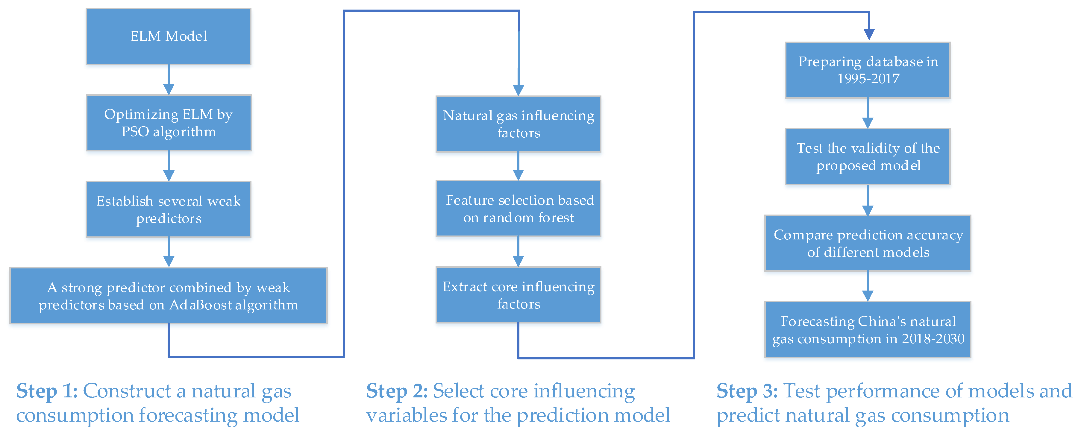
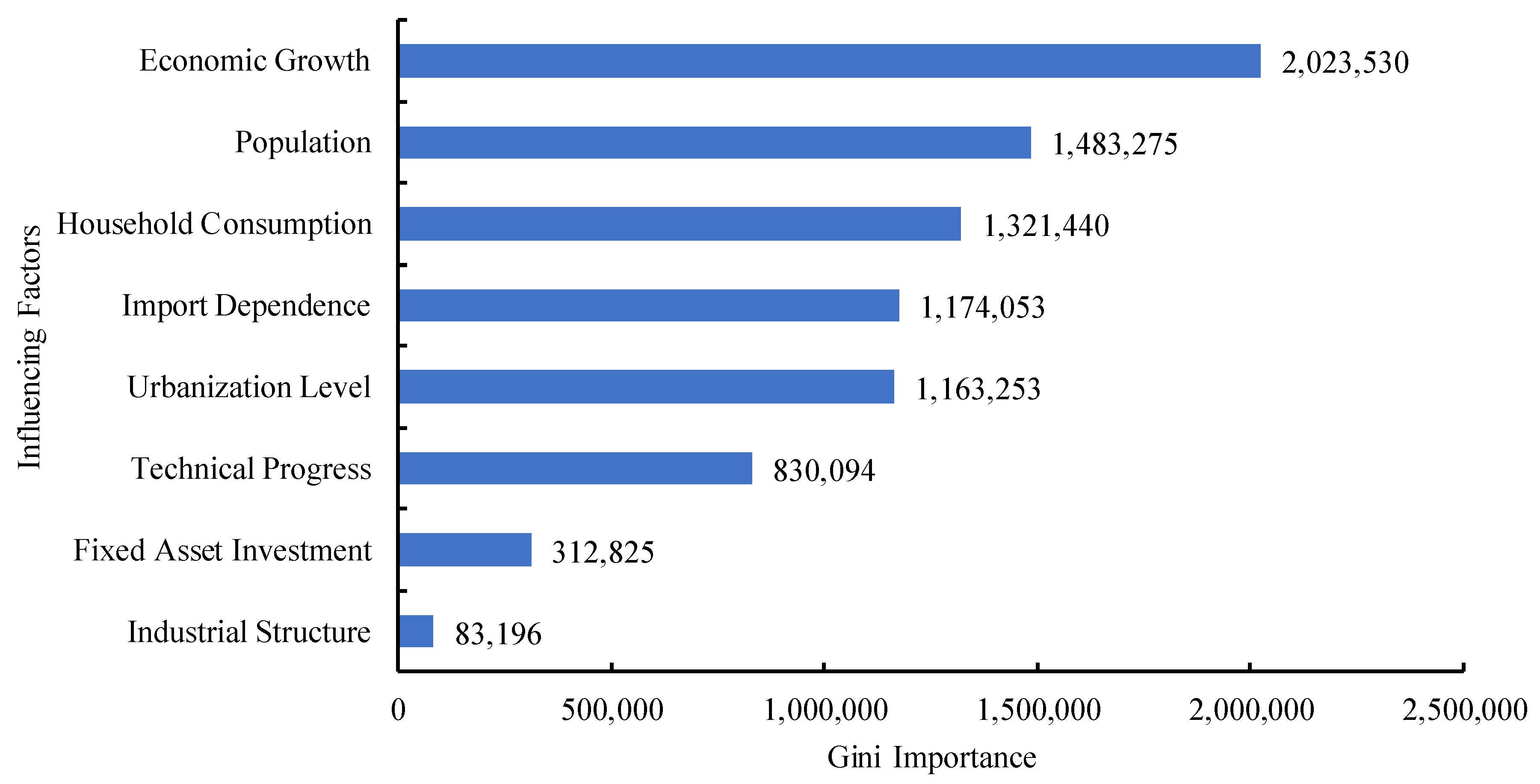
• When analyzing the factors affecting China’s natural gas, this paper considers the factors of previous research and combines the current development status of China’s natural gas consumption, focusing on the unique influencing factors of natural gas consumption, namely import dependence. At the same time, in order to avoid problems such as multi-collinearity and over-fitting, the random forest algorithm is used to calculate the Gini Importance of each factor, and the core factors of China’s natural gas are extracted as the independent variables of the established prediction model.
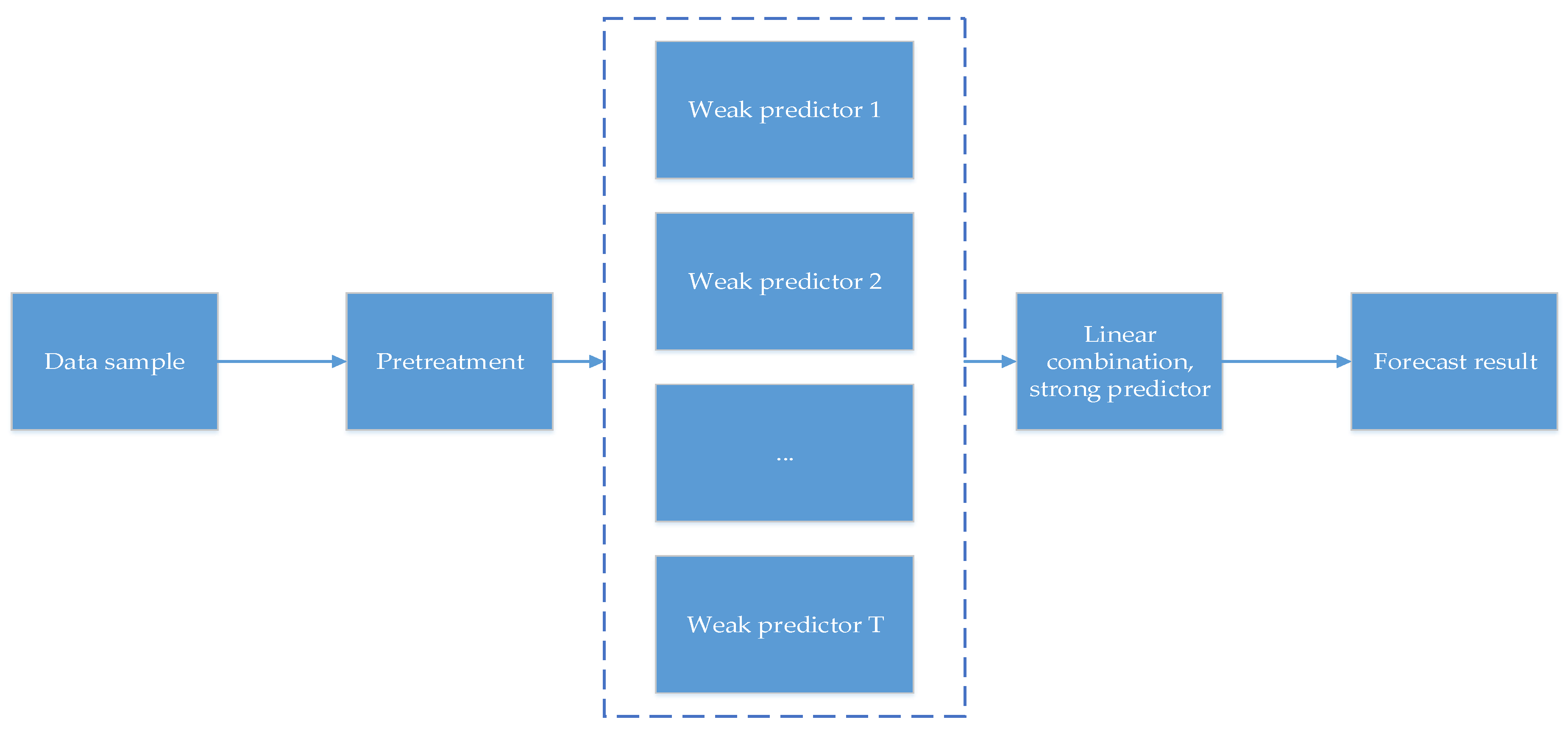
• Based on the advantages of the combined prediction method, this paper uses the PSO algorithm to optimize the input weight matrix and hidden layer deviation of the ELM method, which leads to improvement of the generalization ability of the ELM algorithm. At the same time, the AdaBoost algorithm is used to integrate several weak predictors into a high-precision strong predictor, and the Chinese natural gas consumption prediction model is constructed to further improve the prediction accuracy.
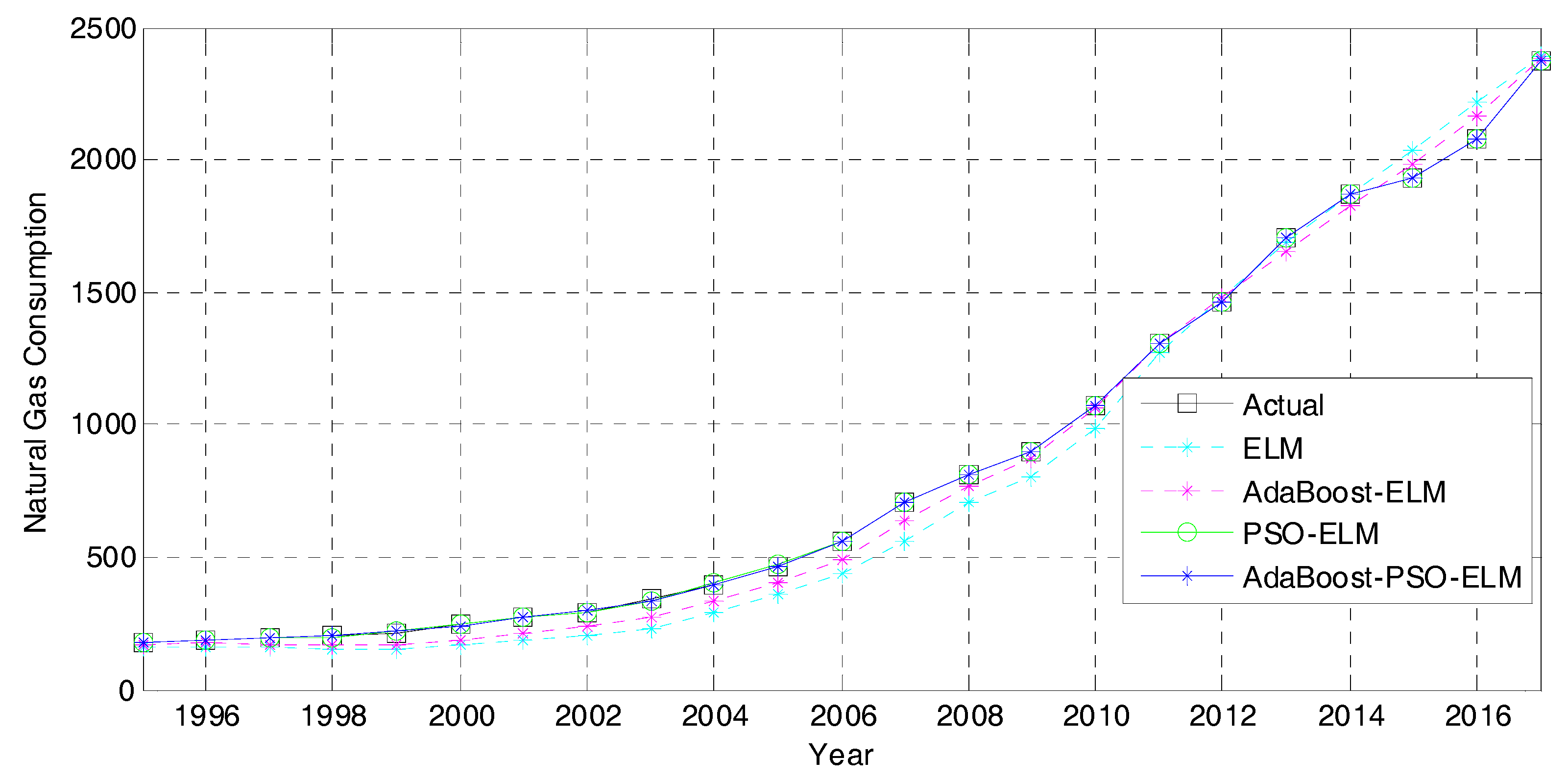
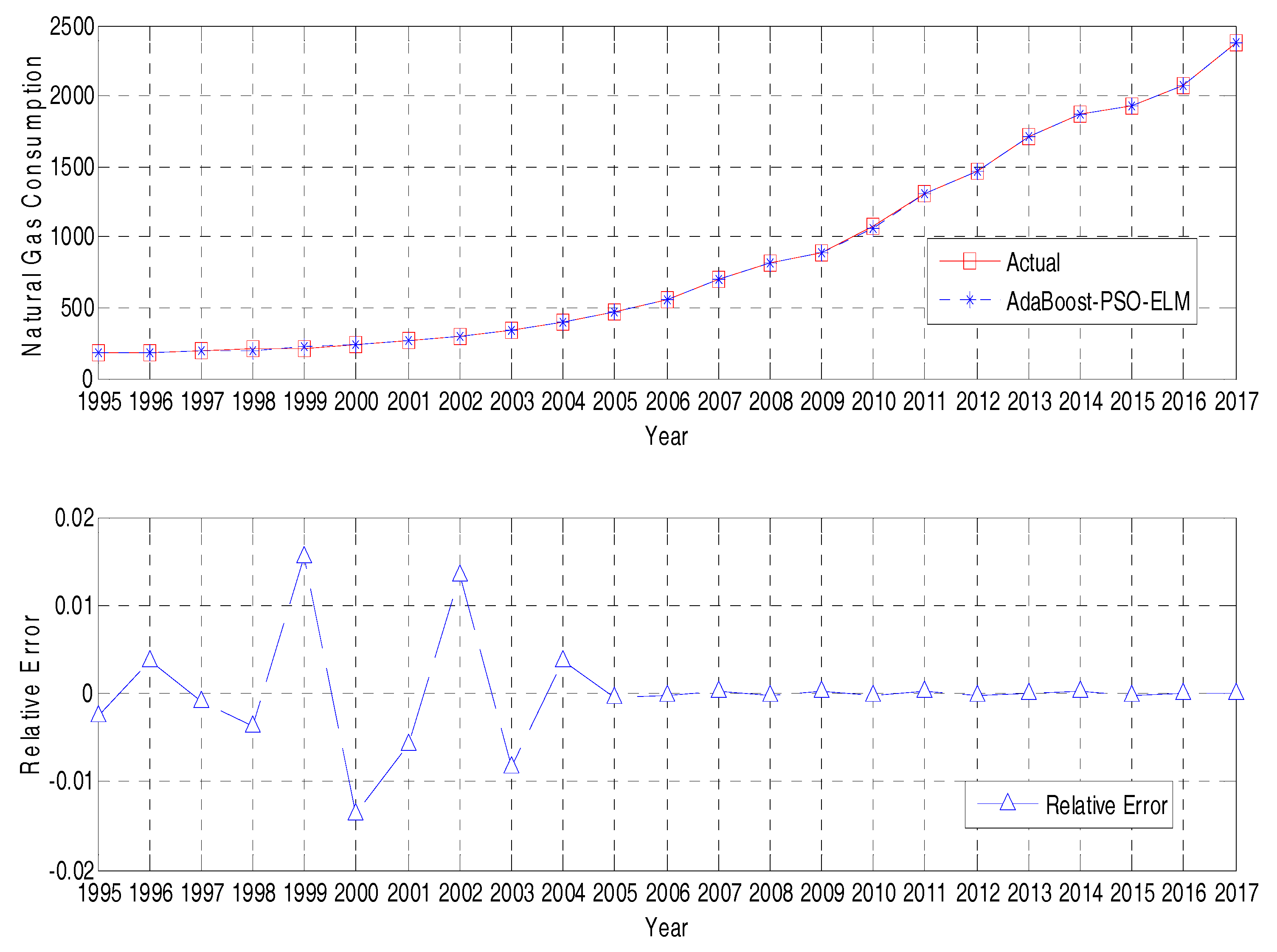
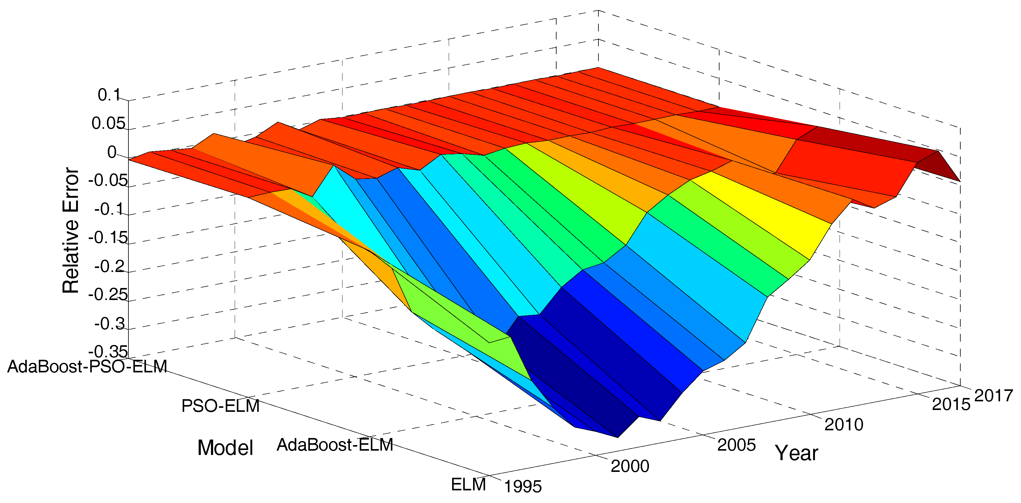
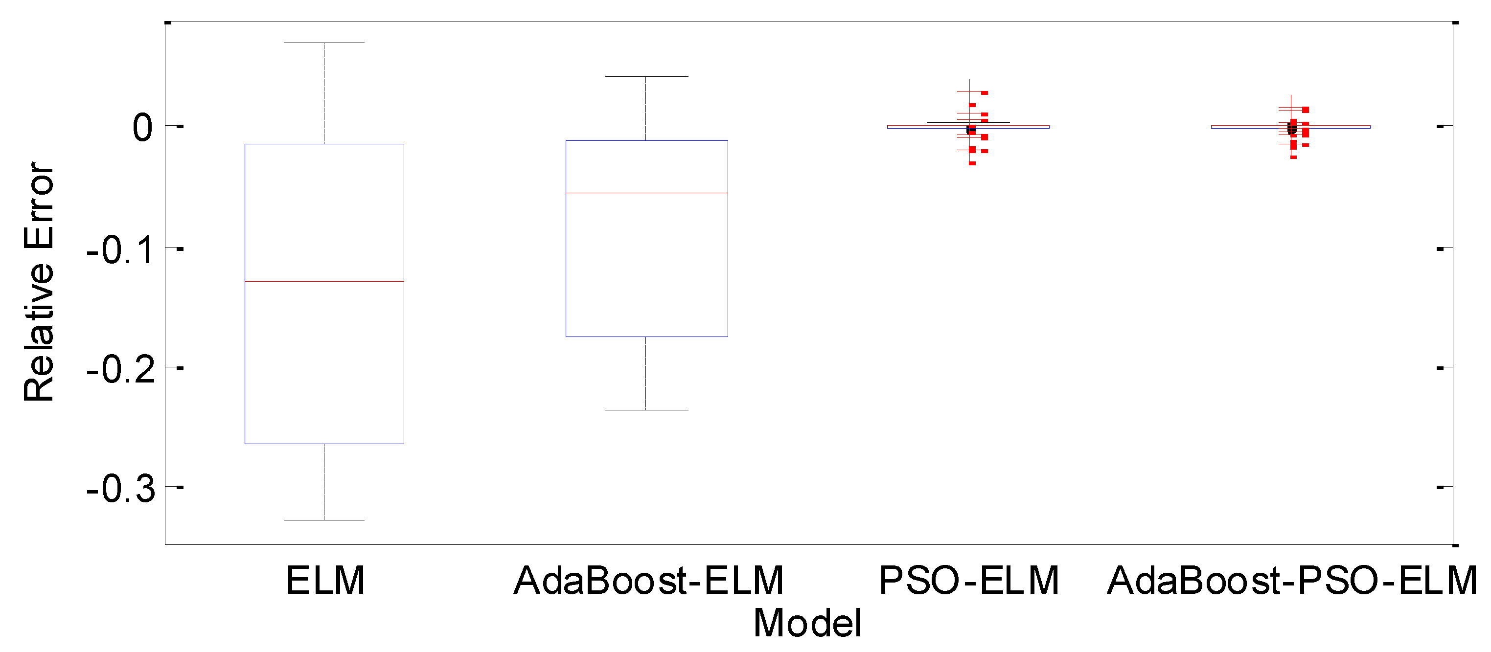
• This paper verifies the superiority of the AdaBoost-PSO-ELM method by comparing the relative error and prediction accuracy of PSO-ELM, AdaBoost-ELM and ELM. Then combined with the prediction model training parameters and the time series prediction results of each core influencing factors, the trend of natural gas consumption in 2018–2030 is predicted, which provides a reference for future policy formulation.

The reminder of the paper is organized as follows. In Section 2, we explain the theory of Random Forest algorithm, AdaBoost algorithm, optimizing PSO and improving ELM, and construct the natural gas consumption prediction model based on AdaBoost-PSO-ELM. In Section 3, we analyze the development status of China’s natural gas consumption from different regions and industries, and use the random forest method to extract the core influencing factors of natural gas consumption. Section 4 contains the empirical research and Section 5 summarizes the conclusions of the study.

The flow chart of this study is shown in Figure 1.

2. Methodology

The main methods used for this paper are the Random Forest Algorithm, Extreme Learning Machine, Particle Warm Optimization and AdaBoost algorithm; here, we briefly describe it as follows.

2.1. Random Forest Algorithm

The random forest algorithm was proposed by scholars Leo Breiman and Adele Cutler in 2001 [31,32]. Compared with other methods, it overcomes the problems of local optimal solution and over-fitting. The core idea of the algorithm is to use the bootstrap resampling technique to repeatedly extract some samples from the original training sample set to generate a new training sample set, and then generate multiple decision trees according to the self-service sample set to form a random forest. The decision result of the data is determined by the score formed by the decision tree voting.

In addition, the random forest algorithm has an important feature that can calculate the importance value of each variable. When all training samples are not used, some samples will be left for each sample, called Out of Bag (OOB) [31], which is used to obtain the classification or prediction accuracy of random forests, simplifying the individual test samples. Therefore, when calculating the importance value of a certain predictor, first randomly discard the value corresponding to the variable in the OOB sample set. Then, the accuracy of the random forest before the disorder and the accuracy of the disorder are obtained respectively. By using the difference between the two, the replacement importance value of each variable can be obtained.

Assuming that the original sample content is $N$, and each base variable is $x_1,x_2,\cdots ,x_m$, $b$ new samples are randomly selected by the bootstrap method, and form $b$ classification trees thereby. Samples that have not been sampled constitute out-of-bag data, which can be used as a test sample to assess the importance of each variable in prediction or classification. The process is as follows:

• Using the bootstrap sample to form each decision tree, and predicting or classifying the corresponding OOB, then obtaining the voting score of each sample in the OOB in the $b$ samples, recorded as $rat{e}_1,rat{e}_2,\cdots ,rat{e}_b$;
• Randomly change the value of the variable in the OOB sample to form a new OOB test sample, and then use the established random forest to predict or classify the new OOB. According to the number of correct samples, the voting score of each sample is obtained, namely:

  $$\left[\begin{array}{ccccc}rat{e}_{11}& rat{e}_{12}& rat{e}_{13}& \cdots & rat{e}_{1b}\\ rat{e}_{21}& rat{e}_{22}& rat{e}_{23}& \cdots & rat{e}_{2b}\\ rat{e}_{31}& rat{e}_{32}& rat{e}_{33}& \cdots & rat{e}_{3b}\\ ⋮& ⋮& ⋮& ⋮& ⋮\\ rat{e}_{p1}& rat{e}_{p2}& rat{e}_{p3}& \cdots & rat{e}_{p4}\end{array}\right]$$

  (1)
• Subtracting the $i$-th row vector corresponding to the matrix (1) by $rat{e}_1,rat{e}_2,\cdots ,rat{e}_b$, summing the average and then dividing by the standard error to obtain the importance score of the variable $X_i$, namely:

  $$scor{e}_i=({\displaystyle \sum _{j=1}^b(rat{e}_j-rat{e}_{ij})/}b)/S_E,(1\le i\le p),$$

  (2)

2.2. AdaBoost Algorithm

The AdaBoost algorithm was proposed by Schapire and Freund in 1995 and is based on the machine learning algorithm of Boosting [33]. The basic idea is to obtain the training sample weights by repeatedly searching the sample feature space, and it is necessary to constantly adjust the weight of the training samples in the iterative process. The advantage of this algorithm is that it can increase the sample weight with low prediction accuracy and reduce the sample weight with high prediction accuracy, and significantly improve the prediction performance of the whole learning algorithm by linearly combining into a strong predictor [34]. Furthermore, as the AdaBoost algorithm does not have to acquire the lower precision limit of the weak prediction learning algorithm in advance, it is widely used in various practical problems. The specific operation is shown in Figure 2.

2.3. Improved ELM Theory Based on PSO Algorithm

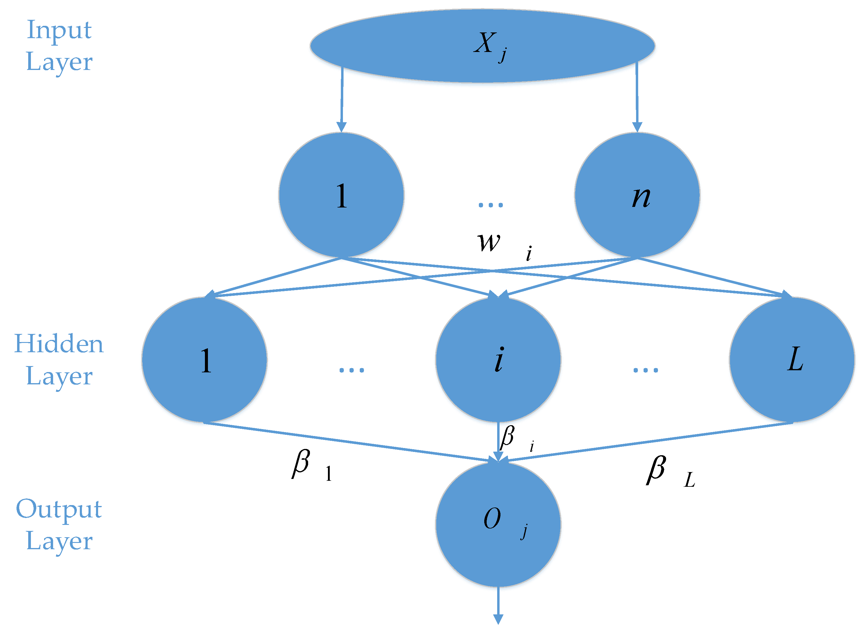
2.3.1. Extreme Learning Machine

ELM, which was proposed by Professor Huang Guangbin, is a fast and efficient single-layer feedforward neural network algorithm [35]. Compared with other traditional algorithms, it has the characteristics of small training error, fast learning speed and simple structure, which makes up for the shortcomings of traditional feedforward neural network and is widely used in many fields [35]. In the actual extreme learning training process, the ELM only needs to determine the number of neurons in the hidden layer. Therefore, without adjusting the connection weight between the input layer neurons and the hidden layer neurons and the bias of the hidden layer neurons, the hidden layer output weight matrix can be calculated. The algorithm flow is shown in Figure 3.

Set N initial training sample as $\left(x_i,t_i\right)$, input sample as $x_i={[x_{i1},x_{i2},\dots ,x_{in}]}^T\in R^n$, and output sample as $t_i={[t_{i1},t_{i2},\dots ,t_{im}]}^T\in R^m$ that contains $L\left(N_0\ge L\right)$ hidden layer nodes and the activation function $g\left(x\right)$, which is

$${\displaystyle \sum _{i=1}^L{\beta }_i{g}_i\left(x_i\right)={\displaystyle \sum _{i=1}^L{\beta }_{i}g\left(w_i\cdot x_j+b_i\right)=o_j,j=1,2,\dots ,N},}$$

(3)

wherein, $w_i={\left[w_{i1},w_{i2},\dots ,w_{in}\right]}^T$ is used to connect the input weight vector of hidden layer nodes and input nodes; ${\beta }_i={\left[{\beta }_{i1},{\beta }_{i2},\dots ,{\beta }_{im}\right]}^T$ is used to connect the output weight vector of hidden layer nodes and output nodes; $b_i$ is bias of the i-th hidden layer node; $w_i\cdot x_j$ is the inner product of $w_i$ and $x_j$.

To minimize the learning outcome output, it needs to meet.

$${\displaystyle \sum _{j=1}^N\Vert o_j-t_j\Vert =0},$$

(4)

Thus, the existence of ${\beta }_i,w_i$ makes the formula (4).

$${\displaystyle \sum _{i=1}^L{\beta }_{i}g\left(w_i\cdot x_j+b_i\right)=t_j,j=1,2,3,\dots ,N},$$

(5)

Then, the formula (5) can transfer to the formula (6).

$$H\beta =T,$$

(6)

$$H\left(w_1,\dots ,w_L,b_1,\dots ,b_L,x_1,\dots ,x_L\right)={\left[\begin{array}{ccc}g\left(w_1\cdot x_1+b_1\right)& \dots & g\left(w_L\cdot x_1+b_L\right)\\ ⋮& \ddots & ⋮\\ g\left(w_1\cdot x_N+b_1\right)& \dots & g\left(w_L\cdot x_N+b_L\right)\end{array}\right]}_{N\times L},\beta ={\left[\begin{array}{c}{\beta }_1^T\\ ⋮\\ {\beta }_L^T\end{array}\right]}_{L\times M},T={\left[\begin{array}{c}{t}_1^T\\ ⋮\\ t_N^T\end{array}\right]}_{N\times M},$$

(7)

wherein, $H$ is the output matrix of the neural network hidden layer nodes, and the i-th column represents the i-th hidden layer node output matrix. And, when the activation function is infinitely differentiable, the input connection weight $w_i$ and the implicit layer bias $b_i$ can be randomly initialized for training and modification, which ensuring the output connection weight $\beta$ the least squares solution, the specific is as follows:

$$\min \Vert H\beta -T\Vert ,$$

(8)

Therefore, in the ELM neural network algorithm, it can randomly input the connection weight $w_i$ and the implicit layer bias $b_i$, and determine the hidden layer output matrix $H$. Meanwhile, after training the ELM neural network, it can be transformed into a linear system $H\beta =T$. Then, the output weight $\beta$ can be determined.

$$\widehat{\beta }=H^{+}T,$$

(9)

where, $H^{+}$ is the Moore–Penrose Generalized Inverse of hidden layer output matrix $H$, and the norm of $\widehat{\beta }$ is the smallest and unique. However, when using the ELM algorithm to predict natural gas consumption, there are two main reasons affecting the fitting error: one is the input layer weight and the other is the hidden layer threshold.

2.3.2. Particle Swarm Optimization

The PSO algorithm was proposed by Kennedy and Eberhart in 1995, and has the characteristics of being quickly converging, easily implemented, with great calculation accuracy [36]. By introducing stochastic searching problems in $D$ dimensional space, objective function maximization and minimization can be solved effectively [36]. In $D$ dimensional space, there are $n$ populations $X=\left(X_1,X_2,\dots ,X_n\right)$ consisting of particles. Each particle $i$ consists of one position vector $x_i=\left(x_{i1},x_{i2},\dots ,x_{iD}\right)$ of the $D$ dimensional space and one velocity vector $v_i=\left(v_{i1},v_{i2},\dots ,v_{iD}\right)$. When particle $i$ searching $D$ dimensional space, the best position $P_{best}^i={\left(P_{best}^{i1},P_{best}^{i2},\dots ,P_{best}^{iD}\right)}^T$ is the local optimal solution, and the best location searched by the whole particle swarm $g_{best}={\left(g_{bsest}^{b1},g_{bsest}^{b2},\dots ,g_{bsest}^{bD}\right)}^T$ is the global optimal solution. The velocities and positions of particles can be obtained by the following formula.

$$v_i\left(t+1\right)=w{v}_i\left(t\right)+c_1{v}_1\left(P_{best}^i\left(t\right)-x_i\left(t\right)\right)+c_2{v}_2\left(P_{best}^i\left(t\right)-x_i\left(t\right)\right),$$

(10)

$$x_i\left(t+1\right)=x_i\left(t\right)+v_i\left(t+1\right),$$

(11)

where,$i=1,2,\dots ,N$, $N$ is the total number of population particles, $w$ is inertia factor. The value of $w$ is nonnegative. When the value is large, the global search ability is strong and the local search ability is weak. When the value is small, the global search ability is weak and the local search ability strong. Dynamic $w$ can get better results. Presently, the most widely used strategy is the linear decreasing weight strategy:

$$w^{\left(t\right)}=\left(w_{ini}-w_{end}\right)\left(i{t}_{\max }-t\right)/i{t}_{\max }+w_{end},$$

(12)

where, $i{t}_{\max }$ is the maximum number of iterations, $w_{ini}$ is the initial inertia weight, and the typical value is $w_{ini}=0.9$. The inertia weight $w_{end}$ is 0.4 when reaching the maximum number of iterations. The range of value of local and global learning factors $c_1,c_2$ is $0\le c_1,c_2\le 2$, usually, $c_1=c_2=2$. $r_1,r_2$ are two random numbers, ranging from 0 to 1. In order to increase the randomness of searching and prevent blind search of particles, the positions and velocities of particles are limited to $\left[-x_{\max },x_{\max }\right],\left[-v_{\max },v_{\max }\right]$. $Pbes{t}_i$ is the local best position of particle $i$ while $gdes{t}_i$ is the global optimal position.

2.3.3. Calculation Steps of PSO Optimizing ELM Algorithm

In order to effectively improve the prediction accuracy of natural gas consumption in this paper, we use PSO to optimize the above two main parameters to determine the fitness function, as follows:

Step1: Determine the parameters of PSO. Based on a given training sample, we can determine population size $N$, maximum evolutionary iterations $M$, linear decreasing inertia factor $w$, and learning factor $c$.

Step2: Determine the fitness function. We generally take the mean square error of the training sample and the simulated fitting value as the fitness function. Since the ELM can approximate the nonlinear function infinitely, the fitness function will lead to over-fitting, which will reduce the generalization ability of the model.

Step3: Initialize the population. Each particle in the population represents a solution, and each particle contains an input weight matrix and threshold vector information. We calculate the initial fitness value of the population $f$, and set it as the historical optimal value of the respective particles $P_{best}^i$. Further, we mark the position of the particle $i$ with the smallest fitness function as the global optimal value. Further, we set the particle position corresponding to the particle $i$ with the smallest fitness function as $P_{best}^i$, and set it as the global optimal value $g_{best}$.

Step4: Update the population. The particle position and velocity are updated according to the particle swarm algorithm. If the particle is in a stagnant state, the particle position and velocity will be reinitialized.

Step5: Update particle history optimal values and global optimal values. We first calculate a new fitness value $f_n$ of $n$-th iteration. If $i$-th particle corresponds to $f_n^i<P_{best}^i$, then $P_{best}^i=f_n^i$, and conversely unchanged. Assume that in this iteration, the particle position corresponding to $j$-th particle with the smallest fitness function is $P_{best}^j$. If $P_{best}^i<g_{best}$, then $P_{best}^i<g_{best}$, otherwise the global optimum value remains unchanged.

Step6: The iteration ends. When the iterative end condition is satisfied, the iteration is stopped. At this time, the particle corresponding to the global optimal value is the input weight and threshold of the optimal hidden layer node.

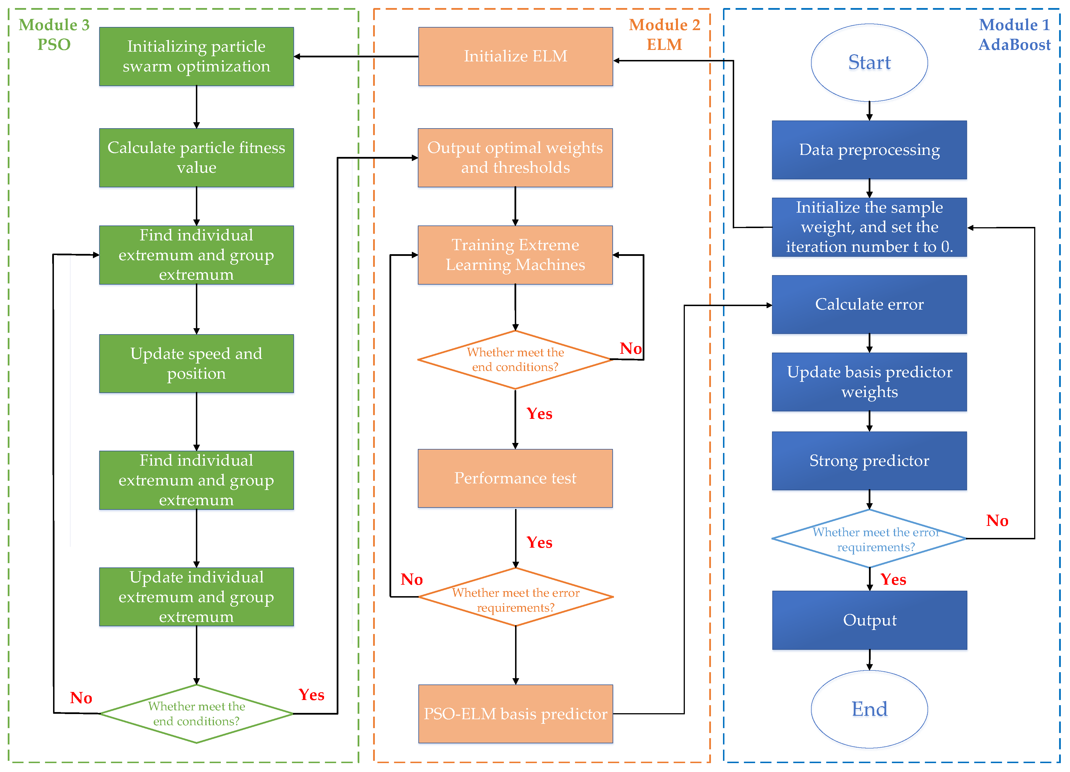
2.4. Establishing Natural Gas Consumption Forecasting Model based on AdaBoost-PSO-ELM Integrated Learning

The natural gas consumption prediction model includes two stages: In the first phase, we use PSO to optimize the input layer weight and the hidden layer threshold of ELM to overcome the lack of generalization ability of the ELM. In the second phase, we use PSO-ELM to build weak predictors. Then, AdaBoost is used to combine several weak predictors with poor prediction effects into strong predictors with better prediction effects.

Suppose there are $N$ training samples $S=\left\{\left(x_i,y_i\right)|i=1,2,\dots ,N\right\}$, there are $T$ predictors output function $f_t\left(x\right),t=1,2,\dots ,T$ trained by PSO-ELM base predictor. Then we can get a strong predictor consisting of $T$ base predictors through AdaBoost. The calculation steps are as follows:

Step1: Initialize the weights of $N$ training samples, sample $D_1$ tends to be uniformly distributed:

$$D_1\left(i\right)=\raisebox{1ex}{$1$}\!\left/ \!\raisebox{-1ex}{$N$}\right.,$$

(13)

where $D_t\left(i\right)$ represents the weight assigned to the sample $\left(x_i,y_i\right)$ in the $t$-th iteration.

Step2: According to the sample distribution $D_t,t=1,2,\dots ,T$, we use Bootstrap to sample training set $S$ and get $S_t$. We train the $t$-th PSO-ELM weak predictor according to the above sample, and then use the trained PSO-ELM to predict the output value of the training data. The absolute value of the weak prediction error is as follows,

$$E_i=\Vert f_t\left(x_i\right)-y_i\Vert ,$$

(14)

Step3: Calculate the weight coefficient of the weak predictor $w_t$ based on ${\epsilon }_t$,

$${\epsilon }_t={\displaystyle {\sum }_{i:e_i>\varphi }{D}_t\left(i\right),i=1,2,\dots ,N},$$

(15)

$$w_t=\frac{1}{2}\ln \frac{1-{\epsilon }_t}{{\epsilon }_t},$$

(16)

Step4: Adjusting the weight of the next round of training samples according to the weight coefficient $w_t$,

$$\begin{array}{l}{D}_{t+1}\left(i\right)=\{\begin{array}{c}\frac{\exp \left(w_t\right)\times D_t\left(i\right)}{Z_t},e_i>\varphi \\ \frac{\exp \left(-w_t\right)\times D_t\left(i\right)}{Z_t},e_i\le \varphi \end{array},\end{array}$$

(17)

where, $\varphi$ is the prediction error threshold and $Z_t$ is the normalization factor.

Step5: After training $T$ rounds, we get $T$ weak predictor functions based on PSO-ELM. Then, we combine them to get strong predictor functions,

$$F\left(x\right)={\displaystyle \sum _{t=1}^T{w}_t\times f_t}\left(x\right),$$

(18)

In summary, after several weak predictors are repeatedly updated and adjusted in our framework, a strong predictor is formed, which is natural gas consumption prediction model based on AdaBoost-PSO-ELM integrated learning. The specific framework and process are shown in Figure 4.

3. Extraction of Core Factors Affecting Natural Gas Consumption

Based on the study of natural gas consumption in different regions and industries in China, this paper combines literature analysis, economic meaning and random forest algorithm to extract the core influencing factors of natural gas consumption as the independent variables of the later prediction model.

3.1. Analysis of Current Natural Gas Consumption

Along with the changing of China’s clean energy consumption structure, total natural gas consumption has grown rapidly, and China has gradually constructed the natural gas supply system of “West-to-East Gas Transmission, North-to-South Gas Transmission, Sea-to-Air Landing and Liquefaction Point Supply” [5,6]. As natural gas has the characteristics of being high quality, clean, and highly efficient, its proportion in primary energy consumption is increasing [5,6]. At the same time, China has entered a stage of high development of industrialization and urbanization, resulting in rising energy demand. Therefore, according to the China Energy Statistical Yearbook (2017), China’s natural gas consumption has shown a rapid growth trend from different provinces and different industries [4].

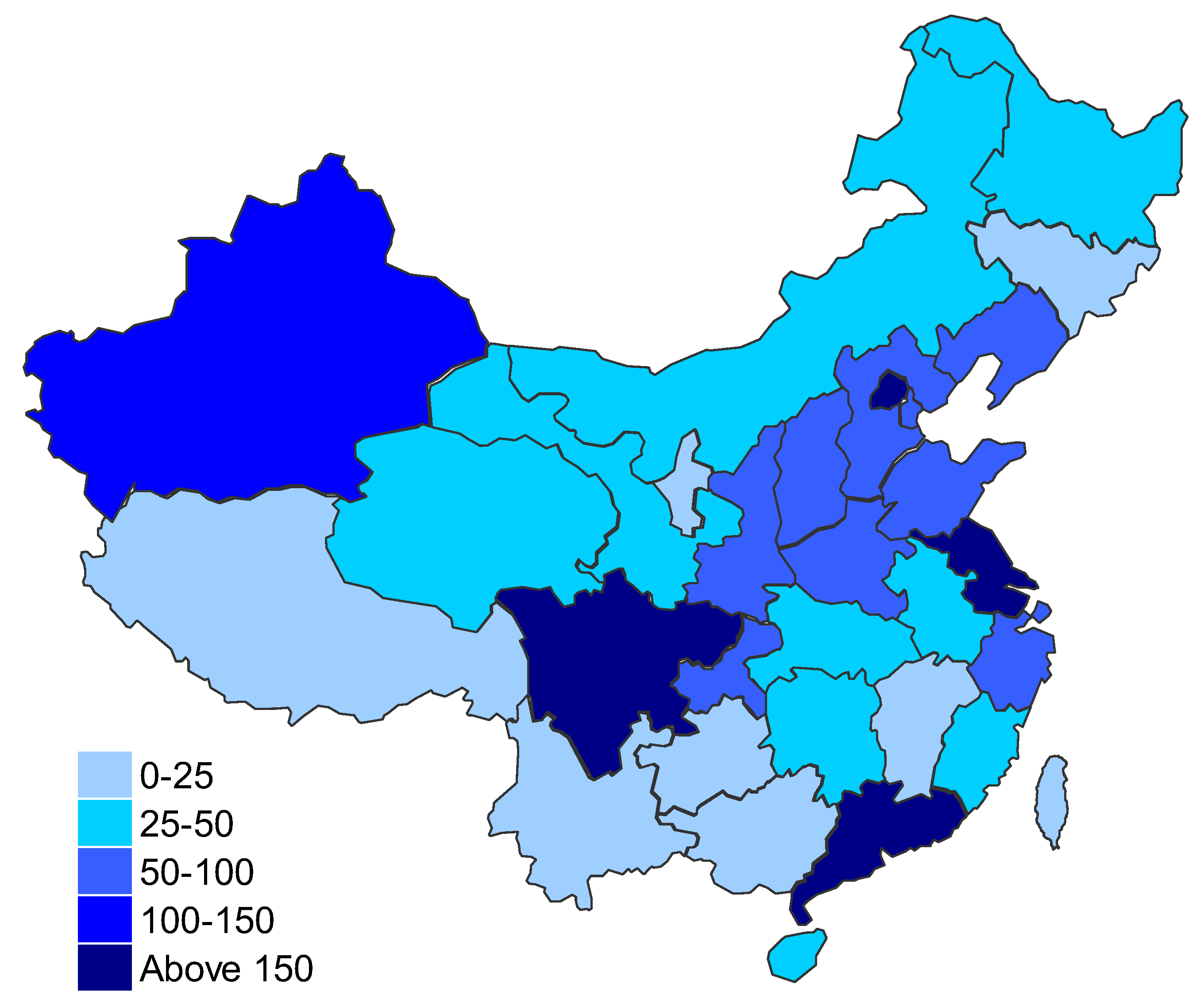
• From the perspective of different provinces, natural gas consumption is mainly in North China, Yangtze River Delta and Pearl River Delta; while Sichuan Province has become the largest consumer of natural gas, as shown in Figure 5.
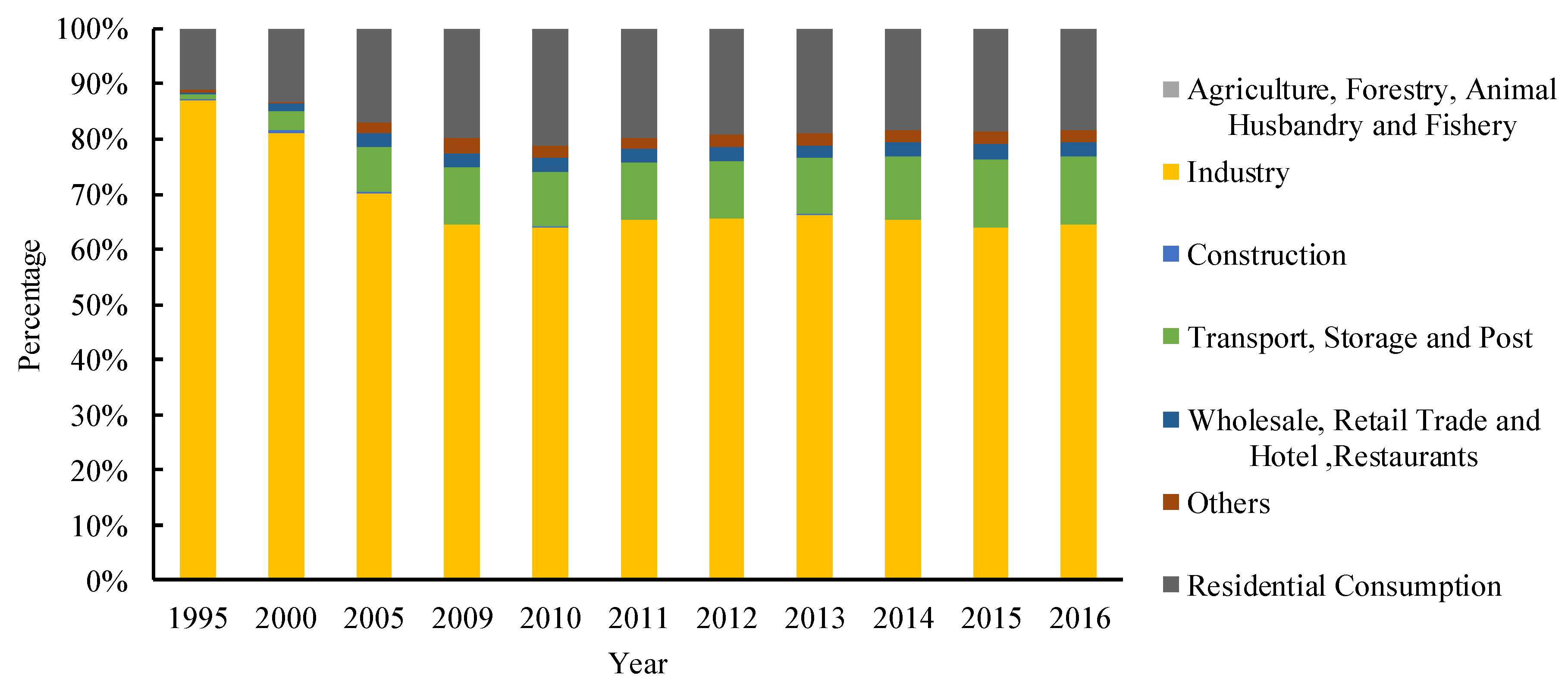
• From the perspective of different industries, the proportion of industrial consumption in total is stable at around 60%, the proportion of residential consumption is stable at around 20%, and the consumption of transportation, storage and post accounts for about 15%; in addition, 5% is used in other industries, as shown in Figure 6.

3.2. Extraction of Core Factors Affecting Natural Gas Consumption

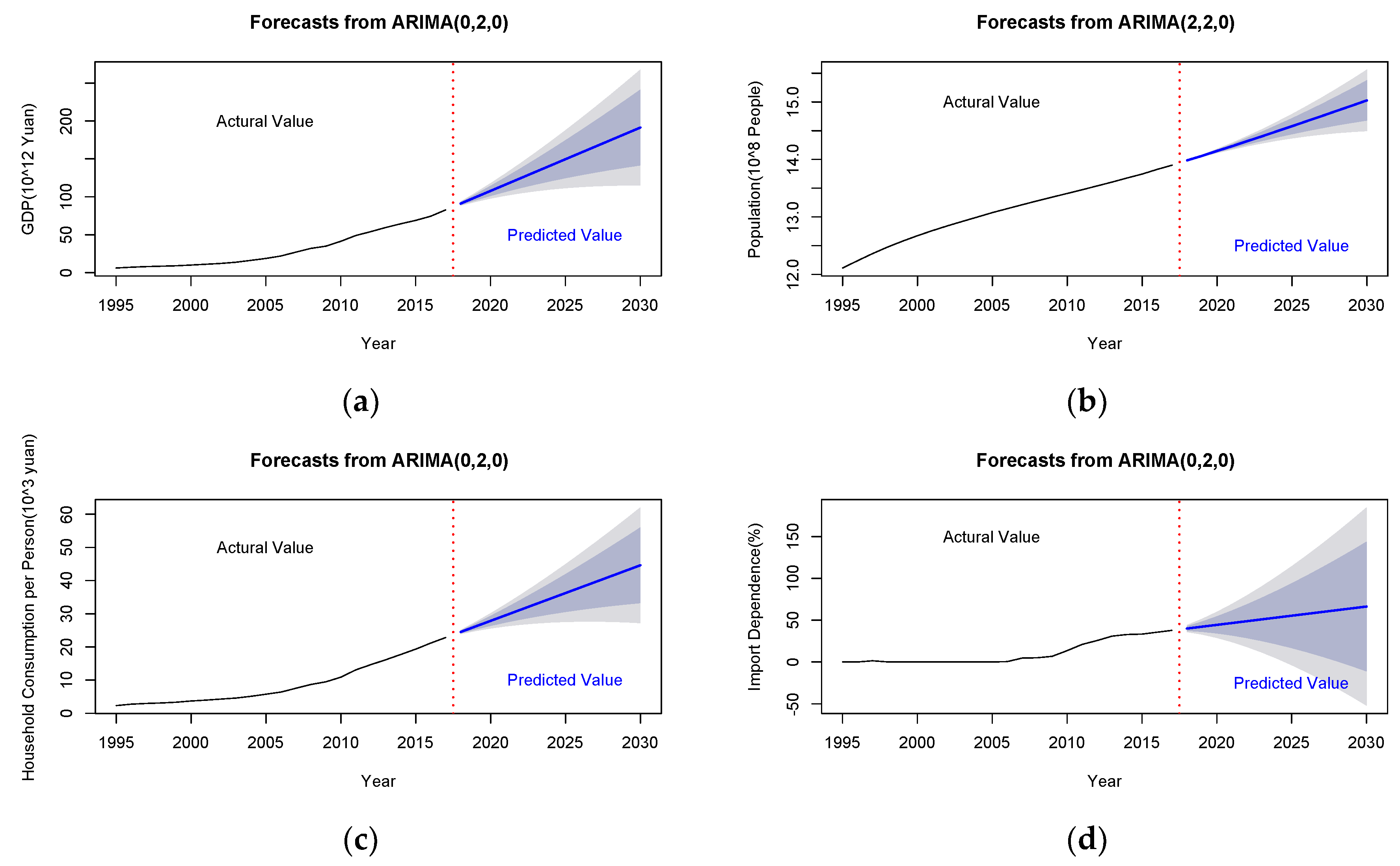
Choosing factors affecting natural gas consumption is the basis of this study. Based on literature analysis and economic implications, we selected eight variables to be further studied, including population, economic growth, urbanization level, industrial structure, household consumption, technological advances, import dependence and fixed asset investment, marked as $x_i,i=1~8$. According to the energy conversion coefficient stipulated by the national standard (GB2589-81), 1 cubic meter of natural gas can be converted into 1.2143 kilograms of standard coal, and we use the electric heating power equivalent calculation method to calculate the natural gas consumption data over the years.

In order to select the core influencing factors, the random forest is used to calculate the importance index of each influencing factor. The concept of the algorithm and the calculation formula of the index have been introduced in Section 2.1. Then, Gini Importance of each independent variable is calculated, which is shown in Figure 7.

Figure 7 is the Gini Importance of each variable calculated from the random forest model. According to Gini Importance, the order of each variable from big to small is $x_2>x_1>x_5>x_7>x_3>x_6>x_8>x_4$. Therefore, we choose the four variables with the largest Gini Importance value as the independent variable, including economic growth, population, household consumption, and import dependence.

• Economic growth ($x_2$): Since mankind entered the industrial era, energy has become an important factor in a country’s economic development and social progress, and it provides the necessary impetus for economic growth. Economic development is inseparable from energy, so economic growth will promote the consumption of natural gas.
• Population ($x_1$): Population is the most fundamental component of the social system, and the consumption of natural gas is generated by people. In the absence of changes in other conditions, the population has a positive relationship with the total demand for natural gas, that is, the larger the population, the greater the demand for natural gas consumption.
• Household consumption ($x_5$): With the continuous improvement of people’s living and consumption levels, the demand for clean energy continues to increase, directly driving the growth of natural gas consumption. At the same time, the negative impact of traditional energy on the ecological environment has prompted changes in the existing energy consumption structure. Therefore, the level of household consumption is a core factor in the consumption of natural gas.
• Import dependence ($x_7$): Import dependence = import quantity/(yield quantity + import quantity − export quantity), the import dependence of natural gas reflects the contradiction between supply and demand of natural gas. Since 2017, due to the tightening of China’s environmental protection policies and the “coal to gas” program, China’s natural gas consumption has been growing rapidly. In the future, China’s natural gas supply gap will still be large, and imported pipeline gas and Liquefied Natural Gas (LNG) will still be important ways to make up for the tightness of the gas source. Therefore, the index of import dependence can be used as a core factor affecting natural gas consumption.

Currently, we choose the four variables with the largest Gini Importance value as the independent variables, the dependent variable is China’s natural gas consumption. At this point, we have chosen the independent and dependent variables, which provide variables for the later prediction models.

4. Empirical Research

4.1. Database

Data of empirical research includes a dependent variable (natural gas consumption), four independent variables (economic growth, population, household consumption, import dependence), and the interval is 1995–2017, as shown in

Table 1. Historical data.

Year	Natural Gas Consumption (108 Cu.m)	GDP (108 Yuan)	Population (104 People)	Household Consumption per Person (Yuan)	Import Dependence (%)
1995	177.41	61,340	121,121	2318	0.13
1996	184.88	71,814	122,389	2750	0.00
1997	195.44	79,715	123,626	2963	1.43
1998	202.57	85,196	124,761	3112	0.13
1999	214.94	90,564	125,786	3332	0.12
2000	245.03	100,280	126,743	3707	0.01
2001	274.30	110,863	127,627	3973	0.00
2002	291.84	121,717	128,453	4288	0.00
2003	339.08	137,422	129,227	4592	0.00
2004	396.72	161,840	129,988	5123	0.00
2005	467.63	187,319	130,756	5754	0.00
2006	561.41	219,439	131,448	6399	0.47
2007	705.23	270,232	132,129	7553	4.68
2008	812.94	319,516	132,802	8685	5.03
2009	895.20	349,081	133,450	9491	6.75
2010	1069.41	413,030	134,091	10,892	13.56
2011	1305.30	489,301	134,735	13,102	21.01
2012	1463.00	540,367	135,404	14,663	25.64
2013	1705.37	595,244	136,072	16,150	30.91
2014	1868.94	643,974	136,782	17,732	32.86
2015	1931.75	689,052	137,462	19,349	33.35
2016	2078.06	743,586	138,271	21,166	35.60
2017	2373.00	827,122	139,008	22,841	37.80

. This paper uses Matlab R2014a for programming, and as for the test platform environment, we use the Intel Core i5-6200U, with 8G memory and the Windows 10 Professional Edition system.

4.2. Natural Gas Consumption Forecasting Based on AdaBoost-PSO-ELM model

4.2.1. Parameter Setting

We used the data from 1995 to 2009 as the training set, and used the data from 2010 to 2017 as the test set. Then we built the AdaBoost-PSO-ELM model for the training set and evaluated the model through the testing set.

The neural network in the PSO-ELM based predictor uses a 4-H-1 type 3-layer structure. The neuron transfer function is the tansig function, and the network learning rule is the gradient descent method. After repeated tests, PSO parameters were set as follows: population number M = 100, local search factor C1 = 2.4, global search factor C2 = 1.6, maximum iteration number T = 50.

Currently, there is no unified theory to select the ELM number of neurons in the hidden layer H. In addition, the increase in the number K of the base predictor can improve the prediction accuracy of the strong predictor, but if K is too large, the time and space cost will increase. Therefore, we use the empirical formula to select H = 20 to train the neural network, and take K = 5 to construct the AdaBoost-PSO-ELM strong predictor.

4.2.2. Forecasting Result

Based on the optimal parameters of the model obtained from the training set and the test set, we use the back substitution method to estimate the training set as well. The comparison between the predicted value and the actual value based on the AdaBoost-PSO-ELM model is shown in Figure 8.

In order to scientifically reflect the credibility of the predicted value relative to the true value, we introduce the Relative Error (RE) $RE=({\widehat{y}}_t-y_t)/y_t$, which is the ratio of the absolute error to the true value expressed as a percentage.

We use the back-generation estimation method to estimate the 23 sets in the data set. The contrast between the predicted value and the actual value is shown in the top of Figure 8; the line marked by the red box is the real value, and the line of the blue star is the prediction. The value; the relative error is shown in the bottom of Figure 8, where the blue dashed line indicates the predicted relative error for each sample.

The results show that the predicted trend of natural gas consumption and the actual trend of the AdaBoost-PSO-ELM model are basically consistent. At the same time, as the number of iterations increases, the prediction effect of the strong predictor is continuously improved. The natural gas consumption forecasting relative error is controlled within 0.02%, which effectively validates the prediction accuracy and reliable robustness of AdaBoost-PSO-ELM.

4.3. Discussion

4.3.1. Relative Error Analysis

Next, we compare the predicted performance of four different models, including a single ELM model without weight and threshold optimization, and AdaBoost-ELM (with integrated learning), PSO-ELM (with weight and threshold optimization) and AdaBoost-PSO-ELM (with integrated learning, weight and threshold optimization).

First, we compare the relative errors between different models, which are shown in Figure 9 and Figure 10.

It can be seen from Figure 9 and Figure 10 that the prediction trends of the four prediction models are basically the same, and the relative errors of the various prediction models will gradually decrease over time. The results show that the improvement effect of PSO on ELM is better than that of AdaBoost on ELM, which shows that PSO is more significant for weight optimization than simple integrated learning. The four predictive models are ranked from good to bad: AdaBoost-PSO-ELM> PSO-ELM> AdaBoost-ELM> ELM.

To show the forecasting accuracy of each model more intuitively, we use the boxplot to compare the relative errors of each forecasting model. The boxplot displays the following five statistics of the relative error for each forecasting model: the minimum, first quartile, the median, third quartile and the maximum. The boxplot of relative errors for different models are shown in Figure 11.

As shown in Figure 11, the relative error of the AdaBoost-PSO-ELM model forecasting result is the smallest, followed by PSO-ELM model, and the relative error of ELM is the largest.

4.3.2. Prediction Accuracy Analysis

In order to further compare the performance of different models, four statistical indicators of the prediction model were calculated, including, Goodness of Fit (R²), Mean Square Error (MSE), Mean Absolute Error (MAE) and Mean Absolute Percentage Error (MAPE). The calculation equations of the indexes are as shown in Equations.

$$R^2=\frac{SSR}{SST}={\displaystyle \sum _{i=1}^N({\widehat{y}}_i}-{\overline{y}}_i{)}^2/{\displaystyle \sum _{i=1}^N{(y_i-{\overline{y}}_i)}^2},$$

(19)

$$MSE=\frac{1}{N}\sqrt{{\displaystyle \sum _{t=1}^N{({\widehat{y}}_t-y_t)}^2}},$$

(20)

$$MAE=\frac{1}{N}{\displaystyle \sum _{t=1}^N\left|{\widehat{y}}_t-y_t\right|},$$

(21)

$$MAPE=\frac{1}{N}{\displaystyle \sum _{t=1}^N\left|({\widehat{y}}_t-y_t)/y_t\right|},$$

(22)

The results are shown in

Table 2. The calculation results of the four models.

Model	R2	MSE	MAE	MAPE
ELM	0.9637	41.8220	17.4555	0.0467
AdaBoost-ELM	0.9969	29.3581	12.0851	0.0292
PSO-ELM	0.9999	0.8624	0.2470	0.0008
AdaBoost-PSO-ELM	0.9999	0.8435	0.2379	0.0008

.

The prediction accuracy of AdaBoost-ELM is much better than that of a single ELM, indicating that AdaBoost can improve the prediction effect through integrated learning. The weight and threshold optimization through PSO is better than the unoptimized model prediction, which indicates that PSO can effectively optimize the ELM neural network and improve the prediction effect of the model. Through the model comparison, the prediction significance of the AdaBoost-PSO-ELM model is further verified.

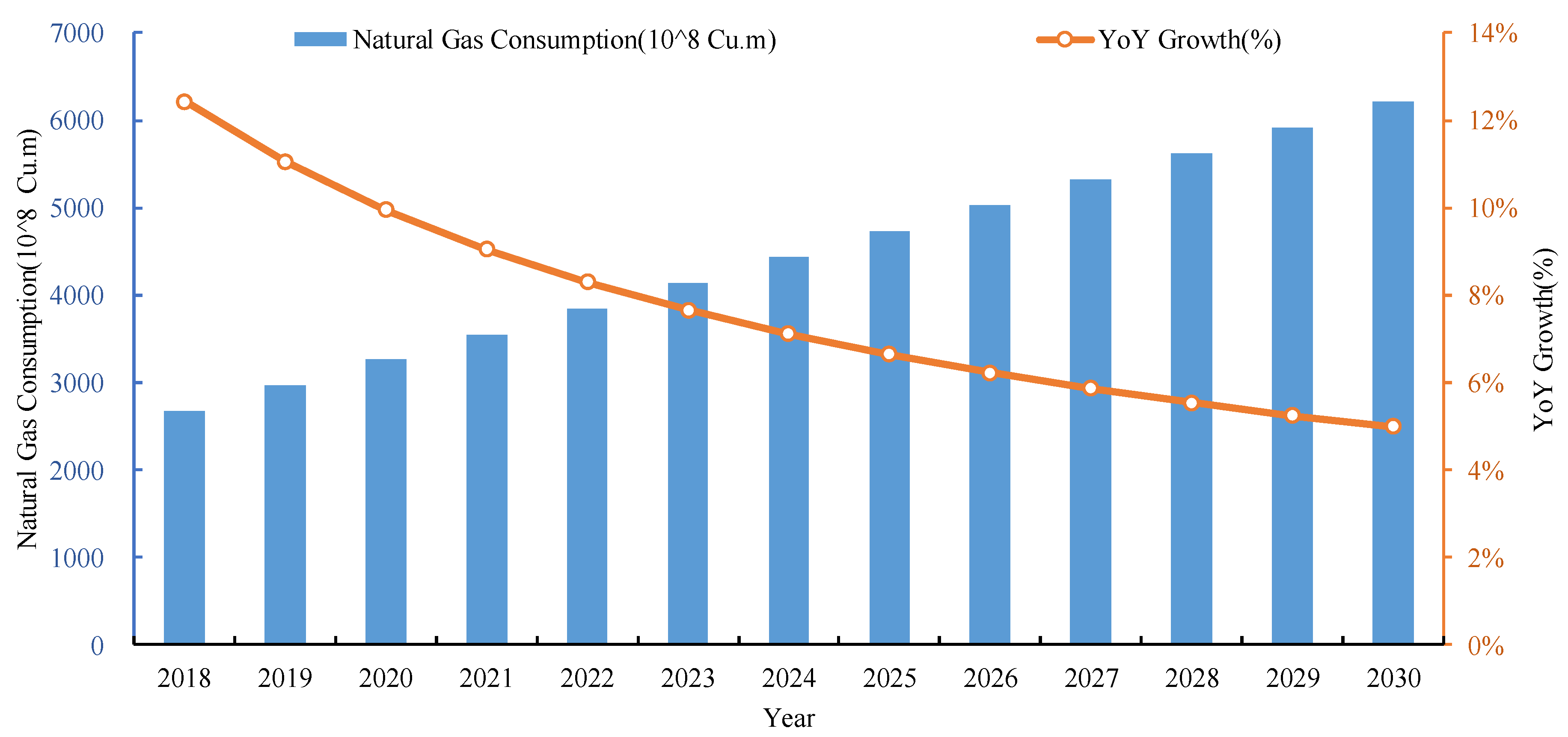
4.4. Prediction of Future Trends

The above shows that the AdaBoost-PSO-ELM model we used has outstanding performance. If we want to predict the future consumption of natural gas through this model, we must predict the future trend of the independent variable first. Based on the data from 1995 to 2017, the core influencing factors of natural gas from 2018 to 2030 are predicted by Autoregressive Integrated Moving Average Model (ARIMA) in time series forecasting method, as shown in Figure 12. The parameters of the ARIMA model are selected according to the characteristics of each variables

Based on AdaBoost-PSO-ELM prediction model and using the best parameters trained above, we forecast the natural gas consumption in the coming 2018–2030, as shown in Figure 13.

With the continuous development of China’s energy revolution, the utilization rate of natural gas is increasing year by year. At present, China’s natural gas supply and demand market is in a balanced state, and the growth of natural gas consumption shows a stable development trend. According to our prediction, the average growth rate of China’s natural gas consumption will reach 7.68% in 2018–2030, which will provide a basis for the designation of gas-related policies.

5. Conclusions

This paper proposed a natural gas consumption prediction model based on AdaBoost-PSO-ELM integrated learning, which transformed several weak predictors into strong predictors with strong prediction effects through the PSO optimizing ELM method. In order to avoid double collinearity and over-fitting, the random forest algorithm was used to extract the core factors of China’s natural gas as the independent variables of the prediction model. Finally, the natural gas related data from 1995 to 2017 were selected and the results were as follows: (1) In the process of extracting the core influencing factors, the combination of economic meaning analysis and random forest was used as the basis to determine the independent variables needed for the prediction model. (2) Using the PSO algorithm to optimize the input layer weight and the hidden layer threshold in the ELM algorithm could effectively improve the prediction performance. (3) Comparing the R2, RSE, MAE and MAPE values under the PSO-ELM, AdoBoost-ELM and ELM methods, it proved that the AdaBoost-PSO-ELM integrated learning method had significant advantages; (4) Based on AdaBoost-PSO-ELM forecasting model, China’s natural gas consumption and the future development of core influencing factors from 2018 to 2020 were further predicted. The above results showed that the AdaBoost-PSO-ELM integrated learning prediction method proposed in this paper was effective and feasible, which could further improve the prediction accuracy and provide ideas for subsequent related research.

In reality, the stochastic fluctuations in natural gas consumption are complex and diverse. By using scientific prediction methods to predict natural gas consumption, it is possible to grasp the growth trend of natural gas consumption. It will provide a quantitative reference for government departments to formulate natural gas industry policies and natural gas infrastructure investment plans, and help government to intervene in advance to balance the contradictions that may arise in the supply and demand of the market.

References

1. Dong, X.C.; Pi, G.L.; Ma, Z.W.; Dong, C. The Reform of the Natural Gas Industry in the PR of China. Renew. Sustain. Energy Rev. 2017, 73, 582–593. [Google Scholar] [CrossRef]
2. Zeng, B. Forecasting the Relation of Supply and Demand of Natural Gas in China During 2015–2020 Using a Novel Grey Model. J. Intell. Fuzzy Syst. 2017, 32, 141–155. [Google Scholar] [CrossRef]
3. Zhang, Y.; Ji, Q.; Fan, Y. The Price and Income Elasticity of China’s Natural Gas Demand: A Multi-Sectoral Perspective. Energy Policy 2018, 113, 332–341. [Google Scholar] [CrossRef]
4. BP Statistical Review of World Energy. Available online: https://www.bp.com/zh_cn/china/reports-and-publications.html (accessed on 20 October 2018).
5. National Development and Reform Commission, National Energy Administration. China’s Energy Development “13th Five-Year Plan”. Available online: http://www.ndrc.gov.cn/zcfb/zcfbtz/201701/t20170117_835278.html (accessed on 20 October 2018).
6. National Development and Reform Commission. China’s Natural Gas Development “13th Five-Year Plan”. Available online: http://www.ndrc.gov.cn/fzgggz/fzgh/ghwb/gjjgh/201706/t20170607_850207.html (accessed on 20 October 2018).
7. Das, A.; McFarlane, A.A.; Chowdhury, M. The Dynamics of Natural Gas Consumption and GDP in Bangladesh. Renew. Sustain. Energy Rev. 2013, 22, 269–274. [Google Scholar] [CrossRef]
8. Li, J.C.; Dong, X.C.; Shangguan, J.X.; Li, J.; Hook, M. Forecasting the Growth of China’s Natural Gas Consumption. Energy 2011, 36, 1380–1385. [Google Scholar] [CrossRef]
9. Xu, G.Z. Analysis of factors affecting China’s natural gas consumption based on LMDI. China Coal 2016, 42, 32–37. [Google Scholar]
10. Luo, D.K.; Xu, P. Natural gas demand forecasting based on improved BP. Oil-Gasfield Surf. Eng. 2008, 27, 20–21. [Google Scholar]
11. Wang, D.Y.; Liu, Y.L.; Wu, Z.; Fu, H.X.; Shi, Y.; Guo, H.X. Scenario Analysis of Natural Gas Consumption in China Based on Wavelet Neural Network Optimized by Particle Swarm Optimization Algorithm. Energies 2018, 11, 825. [Google Scholar] [CrossRef]
12. Zhen, Q.; Guo, X.Q.; Yan, Q. Decomposition of natural gas consumption in China based on industry perpective. China Min. Mag. 2018, 2, 50–57. [Google Scholar]
13. Apergis, N.; Payne, J.F. Natural Gas Consumption and Economic Growth: A Panel Investigation of 67 Countries. Appl. Energy 2010, 87, 2759–2763. [Google Scholar] [CrossRef]
14. Gao, J.; Dong, X.C. Stimulating factors of urban gas consumption in China. Nat. Gas Ind. 2018, 3, 130–137. [Google Scholar]
15. Wang, T.; Lin, B.Q. China’s Natural Gas Consumption and Subsidies—From a Sector Perspective. Energy Policy 2014, 65, 541–551. [Google Scholar] [CrossRef]
16. Aguilera, R.F. The role of natural gas in a low carbon Asia Pacific. Appl. Energy 2014, 113, 1195–1800. [Google Scholar] [CrossRef]
17. Fan, G.F.; Wang, A.; Hong, W.C. Combining Grey Model and Self-Adapting Intelligent Grey Model with Genetic Algorithm and Annual Share Changes in Natural Gas Demand Forecasting. Energies 2018, 11, 1625. [Google Scholar] [CrossRef]
18. Wu, L.F.; Liu, S.F.; Chen, H.J.; Zhang, N. Using a Novel Grey System Model to Forecast Natural Gas Consumption in China. Math. Probl. Eng. 2015, 2015, 686501. [Google Scholar] [CrossRef]
19. Zhang, W.; Yang, J. Forecasting Natural Gas Consumption in China by Bayesian Model Averaging. Energy Rep. 2015, 1, 216–220. [Google Scholar] [CrossRef]
20. Shaikh, F.; Ji, Q. Forecasting Natural Gas Demand in China: Logistic Modelling Analysis. Electr. Power Energy Syst. 2016, 77, 25–32. [Google Scholar] [CrossRef]
21. Karade, Y.; Ozdemir, G.; Aydemira, E. Breeder hybrid algorithm approach for natural gas demand forecasting model. Energy 2017, 12, 1269–1284. [Google Scholar] [CrossRef]
22. Szoplik, J. Forecasting of Natural Has Consumption with Artifical Neural Networks. Energy 2015, 85, 208–220. [Google Scholar] [CrossRef]
23. Iranmanesh, H.; Abdollahzade, M.; Miranian, A. Mid-Term Energy Demand Forecasting by Hybrid Neuro-Fuzzy Models. Energies 2012, 5, 1–21. [Google Scholar] [CrossRef]
24. Bai, Y.; Li, C. Daily Natural Gas Consumption Forecasting based on a Structure-Calibrated Support Vector Regression Approach. Energy Build. 2016, 127, 571–579. [Google Scholar] [CrossRef]
25. Kaytez, F.; Taplamacioglu, M.C.; Cam, E.; Hardalac, F. Forecasting Electricity Consumption: A Comparison of Regression Analysis, Neural Networks and Least Squares Support Vector Machines. Electr. Power Energy Syst. 2015, 67, 431–438. [Google Scholar] [CrossRef]
26. Nieto, P.J.G.; Fernández, J.R.A.; Suárez, V.M.G.; Muñiz, C.D.; García-Gonzalo, E.; Bayón, R.M. A hybrid PSO Optimized SVM-based Method for Predicting of the Cyanotoxin Content from Experimental Cyanobacteria Concentrations in the Trasona Reservoir: A Case Study in Northern Spain. Appl. Math. Comput. 2015, 260, 170–187. [Google Scholar] [CrossRef]
27. Barman, M.; Choudhury, N.B.D.; Sutradhar, S. A Regional Hybrid GOA-SVM Model based on Similar Day Approach for Short-Term Load Forecasting in Assam, India. Energy 2018, 145, 710–720. [Google Scholar] [CrossRef]
28. Wei, N.; Li, C.J.; Li, C.; Xie, H.Y.; Du, Z.W.; Zhang, Q.S.; Zeng, F.H. Short-Term Forecasting of Natural Gas Consumption Using Factor Selection Algorithm and Optimized Support Vector Regression. J. Energy Resour. Technol. 2018, 141, 032701. [Google Scholar] [CrossRef]
29. Zeng, Y.R.; Zeng, Y.; Choi, B.; Wang, L. Multifactor-Influenced Energy Consumption Forecasting Using Enhanced Back-Propagation Neural Network. Energy 2017, 127, 381–396. [Google Scholar] [CrossRef]
30. National Development and Reform Commission. Available online: http://www.ndrc.gov.cn/jjxsfx/201809/t20180930_900073.html (accessed on 24 October 2018).
31. Breiman, L. Random forests. Mach. Learn. 2001, 45, 5–32. [Google Scholar] [CrossRef]
32. Jiao, R.H.; Su, C.J.; Lin, B.Y.; Mo, R.F. Short-Term Forecasting by Grey Model with Weather Factor based Correction. Power Syst. Technol. 2013, 3, 720–725. [Google Scholar]
33. Schapire, R.E. The Boosting Approach to Machine Learning: An Overview; Springer: New York, NY, USA, 2003; pp. 149–171. [Google Scholar]
34. Cao, Y.; Miao, Q.G.; Liu, J.C.; Gao, L. Advance and Prospects of AdaBoost Algorithm. Acta Autom. Sin. 2013, 39, 745–758. [Google Scholar] [CrossRef]
35. Li, M.B.; Huang, G.B.; Saratchandran, P.; Sundararajan, N. Fully Complex Extreme Learning Machine. Neurocomputing 2005, 10, 306–314. [Google Scholar] [CrossRef]
36. Couceiro, M.; Ghamisi, P. Particle Swarm Optimization; Springer: New York, NY, USA, 2015; pp. 1–10. [Google Scholar]
Figure 1. The flow chart of this study. ELM: extreme learning machine; PSO: particle swarm optimization.
Energies 11 02938 g001
Figure 2. AdaBoost Algorithm Diagram.
Energies 11 02938 g002
Figure 3. ELM Algorithm Diagram.
Energies 11 02938 g003
Figure 4. Framework Flow Chart of AdaBoost Particle Swarm Optimization Extreme Learning Machine (PSO-ELM) Integrated Learning.
Energies 11 02938 g004
Figure 5. Natural Gas Consumption in China by Province in 2016 (108 cu.m).
Energies 11 02938 g005
Figure 6. China’s Natural Gas Consumption by Industry (%).
Energies 11 02938 g006
Figure 7. The Gini Importance value of each influencing factor of natural gas consumption.
Energies 11 02938 g007
Figure 8. Prediction Performance of AdaBoost-PSO-ELM.
Energies 11 02938 g008
Figure 9. Prediction Performance of Different Models.
Energies 11 02938 g009
Figure 10. Relative Error of Different Models.
Energies 11 02938 g010
Figure 11. The boxplot of relative errors for different models.
Energies 11 02938 g011
Figure 12. Natural gas core influencing factors prediction curve, (a) Forecasting of GDP; (b) Forecasting of Population; (c) Forecasting of Household Consumption per Person; (d) Forecasting of Import Dependence.
Energies 11 02938 g012
Figure 13. Trends of Natural Gas Consumption in 2018–2030.
Energies 11 02938 g013