Compensation for Inverter Nonlinearity in Permanent Magnet Synchronous Motor Drive and Effect on Torsional Vibration of Electric Vehicle Driveline

Abstract

Permanent magnet synchronous motors (PMSMs) with inverters are widely used in electric vehicles (EVs). However, current harmonics caused by the nonlinearity of the inverter generate torque ripples and give rise to torsional vibration in the vehicle driveline. This paper proposes a new compensation method to suppress the torque ripples. This method extracts the 6th-order harmonic component online from the d-axis and q-axis currents with the approximate Fourier transform, and adopts a harmonic current PI regulator to calculate compensation voltage, which is added to the voltage reference to compensate the nonlinearity of the inverter. After correcting the current distortion and improving the motor torque smoothness, the torsional vibration of the driveline caused by the motor pulsating torque is reduced. According to the simulation results, the 6th-order of motor torque ripple and the torsional vibration response is reduced about 26–28%, which confirms the validity of the proposed strategy. The proposed method does not need any additional hardware and can be implemented broadly in PMSM drives.

1. Introduction

Permanent magnet synchronous motors (PMSMs) fed by pulse-width modulated voltage-source inverter (PWM VSI) have been widely used in electric vehicles (EVs), thanks to their high efficiency, high power density and outstanding controllability. However, spatial harmonics of permanent magnet (PM) flux-linkage caused by motor structure and current harmonics resulted from the nonlinearity of the inverter generate undesired torque ripples. Torque ripples delivered by motor give rise to torsional vibration of the driveline and worsen ride comfort.

Techniques for reducing torque ripples caused by the divergence from ideal motor structure are reviewed in [1]. These methods are classified into two main categories. One is motor design optimization, which is the most effective means to minimize torque ripples. The other is active-control technique. This paper does not discuss how to smooth the torque ripples generated by motor structure. Interested readers may refer to the related literatures.

Another source of torque ripples is current harmonics which mainly result from the inverter output voltage error. Because of the finite turn-on/turn-off time of the PWM inverter, it is necessary to insert dead time into gate signal to avoid simultaneous conduction of two switching devices in the same leg of inverter. Moreover, practical switching devices and diodes have voltage drops. All these factors lead inverter output voltage to diverge from the reference voltage, which is known as dead-time effect [2,3]. The error voltage causes distortion of phase voltage and phase current. In other words, phase current has both fundamental component and higher harmonic components, eventually resulting in torque pulsation and deterioration of control performance. Approaches to solve the problem caused by the nonlinearity of the inverter can be divided into three major categories.

One is to modify the PWM width directly or to cancel the blanking time without shoot-through of the direct current (DC) source, while detecting the polarity of phase current with additional hardware [3,4,5]. By inhibiting switching signals for each device according to the direction of current, the resulting output voltage coincides with the ideal voltage waveform. In [3], with the supplementary current sensor, a compensation method is presented to modify the reference wave and combine the PWM signals. Reference [4] adjusts the symmetric PWM pulses and corrects each pulse accordingly to compensate the dead-time effect with the information of current direction. Instead of additional hardware, [5] uses an instantaneous back calculation of the phase angle of the current to detect the current polarity, making the dead-time compensation technique simple and low-cost. Though the approaches above eliminate the blanking time, voltage and current distortion still exist because of device turn-on/turn-off time and voltage drops.

Another approach is to compensate the voltage with the estimation of the instantaneous value or average value of the inverter disturbance. The estimated disturbance voltages are fed back to the voltage reference in order to create a modified voltage. Compensating voltages calculated based on the inverter model is most widely used, which are typically average values of the inverter disturbance during an electrical period. Reference [6] calculates the compensating voltages with the dead time, switching period, current command and DC link voltage to correct the distorted voltage in the synchronous frame. To increase the accuracy of the disturbance voltage compensation, turn-on/off time and voltage drops of power devices are taken into account [7,8]. Generally, these methods can only be implemented offline, because it is not practical to measure characteristics of power devices in real time. However, parameters of power devices vary with operating conditions, making it less accurate to compensate the inverter disturbance with offline experiment results [9]. Then, online methods which can estimate inverter disturbance instantaneously are proposed [10,11,12,13]. Reference [10] proposes an online method to compute the disturbance voltage, but it requires additional hardware circuits to detect the zero crossing of phase current. With the assumption that disturbance voltage changes slowly during a sampling interval, [11] presents an online method which uses an open-loop observer based on ideal motor model to estimate the disturbance voltage. Closed-loop observers are proposed and show good experiment results in estimating disturbance which needs to tune parameters such as observer gains elaborately [12,13]. In [12], a disturbance observer based on the model reference adaptive system (MRAS) is proposed, which considers the parameter uncertainty caused by the varying operating condition of a PMSM. The output voltage of inverter measured by voltage sensors can be used to calculate the disturbance voltage [13], but there are errors due to either the limited sampling frequency of A/D converters or phase lag of filter. Moreover, additional hardware raises the cost of the system.

The third major category of inverter disturbance compensation approach is current harmonic suppression [14,15]. Reference [14] proposes a feed-forward fundamental compensator and a feedback harmonic compensator for the fundamental and the sixth harmonic of the dq-axes currents, respectively. However, the reference current with harmonic component cannot be tracked without error using a proportional–integral (PI) regulator. In [15], a proportional–integral (PI) regulator is used to suppress the sixth harmonic of the d-axis current, thus compensating the distortion of the output voltage resulted from the dead-time effect. The effectiveness of this method is concerned with the gain of integrator.

The PMSM acts as the power source and excites the torsional vibration of the EV driveline as well. Owing to the outstanding controllability of the motor, it is possible to use the motor as the actuator to reduce driveline torsional vibration, which is called active damping control. Torsional vibration of the driveline includes transient-state vibration and steady-state vibration.

Transient-state vibration occurs in driveline when a vehicle quickly accelerates or decelerates. Reference [16] proposes a motor control method to suppress the surge of a hybrid electric vehicle (HEV) in EV mode, which is based on a 2-Degree of Freedom (DOF) powertrain model and uses the motor angular velocity as the feedback signal to modify the motor reference torque. Reference [17] describes a feedback control method to reduce the torsional vibration of an HEV drivetrain, which uses the speed of the motor and the speed of the wheel to calculate the new reference motor torque. To reduce driveline oscillations, [18] proposes a torque estimator and an oscillation controller. The oscillation controller is a third-order linear controller and outputs a damping torque depending on the estimated torque provided by the observer. According to [19], the transient torsional vibration is caused by the quick change of the traction torque, which is especially more severe in an EV than an Internal Combustion Engine (ICE) vehicle, for electric motors have fast torque response. In [20,21], the shaking vibration resulted from the motor torque is suppressed with a feed-forward compensator, and the shaking vibration resulted from the disturbances during vehicle driving such as gear backlash is suppressed with a feedback compensator. As the EV mode of an HEV is similar to an EV, researchers extend the vibration control method to the HEV [22]. In [23], based on a novel filter, the oscillation component of motor speed is extracted, then a proportional controller calculates a corrective torque which is added to the demand torque to create a modified motor reference torque.

Steady-state vibration occurs in driveline when vehicle running at a constant speed, which may create issues of powertrain durability and Noise Vibration and Harshness (NVH) performance, such as shaft durability, gear train rattle and vehicle body boom [24,25]. Steady-state vibration of an EV driveline is mainly excited by motor torque ripples. In [17], to reduce the floor vibration caused by the motor torque ripple, a vibration control method which can reduce the fluctuation of the motor speed is proposed. In [24], to reduce vibration and booming noise of vehicle body of an EV caused by motor torque fluctuations, researchers propose a torque ripple suppression method called programmed current control, which reduces the ripples caused by high-order components of magnetic flux. With this countermeasure, vehicle vibration from start to very low speed EV driving is reduced to an acceptable level. Moreover, motor electromagnetic noise is reduced by 3 to 6 dB. In [25], to reduce the noise of the vehicle cabin of an HEV caused by motor torque ripples, researchers not only optimize the motor design such as air gap configuration, but also superpose harmonic current into phase currents of the motor. The smoothness of motor ripples reduces noise and vibration of the vehicle body by 12 dB, making it possible to realize quiet driving. From the methods above, it is a common practice to reduce steady-state vibration by suppressing motor torque ripples in an EV.

For suppressing vibration, methods to extract frequency and amplitude of interest are needed. The approximate Fourier transform is a method to extract the amplitude of the sine–cosine components of specific frequency [26]. Reference [27] summarizes five methods for decoupling hybrid faults in gear transmission systems, which are Wavelet, Empirical Mode Decomposition, Order Tracking, Sparse Decomposition, and Independent Component Analysis-based decoupling approaches. Since the vibration signals excited by different components are always dependent or correlated, the Bounded Component Analysis technique is proposed. Reference [28] analyzes the vibration data of the bearings in induction motors and gearboxes on the kinematic chain with the Fast Fourier Transform (FFT) and the motor current data with the Power Spectral Density, then extracts the frequencies of interest from a theoretical model. Reference [29] carries out recognition of armature current of DC generator with the FFT, Method of Selection of Amplitudes of Frequencies and Linear Discriminant Analysis. Reference [30] proposes a new method of feature extraction SMOFS-25-EXPANDED (shorted method of frequencies selection-25-Expanded) to analyze the acoustic signals for real incipient states of loaded synchronous motor.

Acquiring accurate model is important in advanced control system design. Model parameter identification is crucial in real application. Reference [31] provides a method to identify parameters of permanent magnet three-phase synchronous motor, which are the direct axis self-inductance, the quadrature axis self-inductance, and the permanent magnet flux linkage.

This paper discusses how to reduce the torque ripple caused by the nonlinearity of the inverter. We propose a dead-time compensation method based on harmonic current suppression, which aims to suppress pulsating torque caused by the nonlinearity of the inverter. This method extracts the 6th-order harmonic component online in the d-axis and q-axis currents resulted from the dead-time effect in real time using the approximate Fourier transform method, and adopts a harmonic current PI regulator to calculate the compensation voltage, which is added to the voltage reference to compensate the dead-time effect. After improving the current distortion and smoothing the motor torque, torsional vibration of the driveline of an EV caused by the motor pulsating torque is reduced. Simulation results confirm the validity of the proposed strategy. The proposed method does not require additional hardware circuits and can be implemented broadly in PMSM drives.

2. Analytical Model of PMSM Torque Ripple

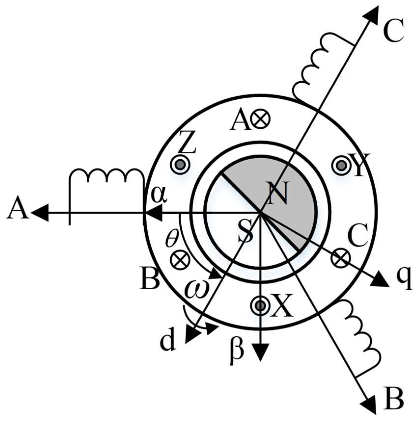
Figure 1 shows the PMSM model and frames used in this paper, where θ and ω are the rotor angle and the stator current vector angular velocity, respectively. The ABC frame is the stationary three-phase frame. The α-β frame is the stationary orthogonal frame, and the d-q frame is a synchronous orthogonal frame.

Voltage equations for the PMSM are described as:

$$\{\begin{array}{l}{u}_{\mathrm{d}}=R_{\mathrm{s}}{i}_{\mathrm{d}}+L_{\mathrm{d}}\frac{\mathrm{d}{i}_{\mathrm{d}}}{\mathrm{d}t}-{\omega }_{\mathrm{r}}{L}_{\mathrm{q}}{i}_{\mathrm{q}}\\ u_{\mathrm{q}}=R_{\mathrm{s}}{i}_{\mathrm{q}}+L_{\mathrm{q}}\frac{\mathrm{d}{i}_{\mathrm{q}}}{\mathrm{d}t}+{\omega }_{\mathrm{r}}(L_{\mathrm{d}}{i}_{\mathrm{d}}+{\mathsf{\lambda }}_{\mathrm{f}})\end{array}$$

(1)

where ω_r is the rotor angular velocity; ${\mathsf{\lambda }}_f$ is the PM flux; R_s is the stator resistance; u_d, i_d, and L_d are the voltage, current, and inductance on the d-axis, respectively; u_q, i_q, and L_q are the voltage, current, and inductance on the q-axis, respectively.

Torque generated by a PMSM is calculated as follows:

$$T=\frac{3}{2}P\left[{\mathsf{\lambda }}_{\mathrm{f}}{i}_{\mathrm{q}}+\left(L_{\mathrm{d}}-L_{\mathrm{q}}\right)i_{\mathrm{d}}{i}_{\mathrm{q}}\right]$$

(2)

where P is the number of pole pairs. If harmonic components in current are not considered, there are no ripple components in the torque of the motor, as shown in Equation (2). However, because of the nonlinearity of the inverter, phase currents contain not only fundamental components but also harmonic components. The effect of the nonlinearity of inverter on the phase current is derived as follows.

In PWM VSI, practical switching devices such as Insulated Gate Bipolar Transistor (IGBT) have finite turn-on/off time. A short time period called “dead time” must be inserted into gating signal to avoid shoot-through of DC link, so the practical gating signal diverges from the ideal one. Besides, switching devices and diodes have on-voltage inevitably. The nonlinearity of the inverter above leads to the inverter output voltage with error. Figure 2 shows the topology of a typical PMSM with three-phase PWM inverter. The basic configuration of the leg of phase A is shown in Figure 3.

Figure 4 presents the gate signal waveforms of ideal and actual inverters, which are obviously different. The difference in gate signals causes inverter output voltage to change, as shown in Figure 5. During the dead time $t_{\mathrm{d}}$, the two switching devices of the same leg of inverter are turned off and the current flows through diodes, i.e., the phase current flows through the diode $D_1/D_2$ if the current direction is negative/positive. Thus, the upper or lower switching device is considered to be turned on, which causes the inverter to output voltage with error. 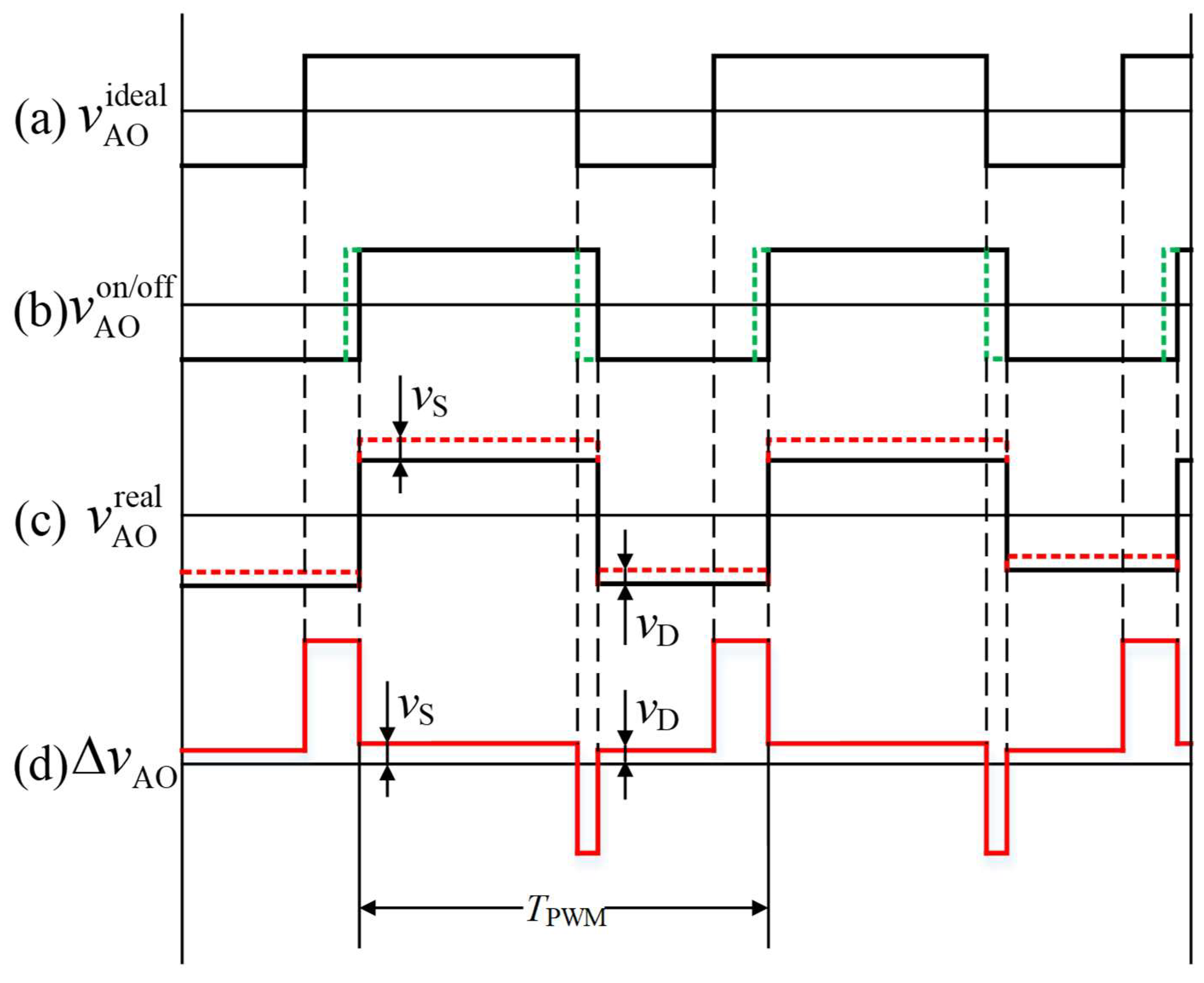Figure 5a shows the ideal output voltage, and Figure 5b,c are the actual output voltage of the inverter. Error voltage is obtained by subtracting actual output voltage from the ideal output voltage, as shown in Figure 5d.

The average inverter output voltage error during one switching period T_PWM can be expressed as Equation (3), which is illustrated in Figure 6.

$$\Delta V_A=\{\begin{array}{l}-\frac{T_{\mathrm{d}}}{T_{PWM}}(V_{\mathrm{dc}}+v_{\mathrm{D}}-v_{\mathrm{S}})-\frac{v_{\mathrm{D}}+v_{\mathrm{S}}}{2},\text{\hspace{0.17em}\hspace{0.17em}}{i}_{\mathrm{A}}<0\\ \frac{T_{\mathrm{d}}}{T_{PWM}}(V_{\mathrm{dc}}+v_{\mathrm{D}}-v_{\mathrm{S}})+\frac{v_{\mathrm{D}}+v_{\mathrm{S}}}{2},\text{\hspace{0.17em}\hspace{0.17em}\hspace{0.17em}\hspace{0.17em}\hspace{0.17em}}{i}_{\mathrm{A}}>0\end{array}$$

(3)

where, T_PWM, $v_{\mathrm{D}}$ and $v_{\mathrm{S}}$ are the switching period of the IGBT, on-voltage of IGBTs and forward voltage of diodes, respectively.

Analyze voltage error as Equation (4) and current error as Equation (5) with Fourier analysis for the case of positive phase current.

$$u_{\mathrm{e}}=\frac{4\Delta V_{\mathrm{A}}}{\mathsf{\pi }}(\cos \omega \mathrm{t}+\frac{1}{5}\cos 5\omega \mathrm{t}+\frac{1}{7}\cos 7\omega \mathrm{t}+\dots \dots )$$

(4)

$$i_{\mathrm{e}}=\frac{u_{\mathrm{e}}}{Z_k}=\frac{4\Delta V_{\mathrm{A}}}{\pi \left|Z_k\right|}[\cos (\omega \mathrm{t}+{\alpha }_1)+\frac{1}{5}\cos (5\omega \mathrm{t}+{\alpha }_5)+\frac{1}{7}\cos (\omega \mathrm{t}+{\alpha }_7)+\dots ]$$

(5)

where,

$$\{\begin{array}{l}{Z}_k=|R_{\mathrm{s}}+jk\omega L_{\mathrm{s}}|=\sqrt{R_{\mathrm{s}}^2+{(k\omega L_{\mathrm{s}})}^2},(k=1,5,7)\\ {\alpha }_k={\tan }^{-1}(\frac{k\omega L_{\mathrm{s}}}{R_{\mathrm{s}}}),(k=1,5,7)\end{array}$$

(6)

$L_{\mathrm{s}}$ is the stator self-inductance of the PMSM.

According to Equations (4) and (5), the voltage errors distorting the phase current consist of fundamental and odd harmonics. Since the three-phase armature windings of a PMSM connect each other by star connection, there are no zero-phase voltages and currents which appear as three times the fundamental frequency. The amplitude of harmonics decreases rapidly as the order increases, and the dominant harmonics are the fifth one and the seventh one in three-phase stationary frame.

Based on the analysis above, the voltage and current in each phase are distorted and contain harmonics caused by the nonlinearity of the inverter. In the three-phase stationary frame, the phase voltage contains the fifth and the seventh harmonics as well as the fundamental components, while the higher-order harmonics are neglected because of their little effect on the inverter output voltage distortion. Voltages in each phase are given as:

$$\{\begin{array}{l}{u}_{\mathrm{A}}=U_1\cos (\omega t+{\delta }_1)+U_5\cos (5\omega t+{\delta }_5)+U_7\cos (7\omega t+{\delta }_7)\\ u_{\mathrm{B}}=U_1\cos (\omega t+{\delta }_1-{120}^{\circ })+U_5\cos (5\omega t+{\delta }_5+{120}^{\circ })+U_7\cos (7\omega t+{\delta }_7-{120}^{\circ })\\ u_{\mathrm{C}}=U_1\cos (\omega t+{\delta }_1+{120}^{\circ })+U_5\cos (5\omega t+{\delta }_5-{120}^{\circ })+U_7\cos (7\omega t+{\delta }_7+{120}^{\circ })\end{array}$$

(7)

where $U_1$, $U_5$, and $U_7$ are the amplitude of the fundamental, the fifth, and the seventh component, respectively. ${\delta }_1$, ${\delta }_5$, and ${\delta }_7$ are the phase of the fundamental, the fifth, and the seventh component, respectively.

Transform the voltage in the three-phase stationary frame to the synchronous reference frame as:

$$\left[\begin{array}{c}{u}_{\mathrm{d}}\\ u_{\mathrm{q}}\end{array}\right]=C_{\mathrm{ABC}/\mathrm{dq}}\left[\begin{array}{c}{u}_{\mathrm{A}}\\ u_{\mathrm{B}}\\ u_{\mathrm{C}}\end{array}\right]$$

(8)

where C_ABC/dq is the transformational matrix from ABC frame to dq frame as follows.

$$C_{\mathrm{ABC}/\mathrm{dq}}=\sqrt{\frac{2}{3}}\left[\begin{array}{ccc}\cos \theta & \cos (\theta -{120}^{\circ })& \cos (\theta +{120}^{\circ })\\ -\sin \theta & -\sin (\theta -{120}^{\circ })& -\sin (\theta +{120}^{\circ })\end{array}\right]$$

where $\theta ={\displaystyle \int {\omega }_{\mathrm{r}}\mathrm{d}t}+{\theta }_0$ is the rotor position.

The transformational matrix from dq frame to ABC frame is,

$$C_{\mathrm{dq}/\mathrm{ABC}}=\sqrt{\frac{2}{3}}\left[\begin{array}{cc}\cos \theta & -\sin \theta \\ \cos (\theta -{120}^{\circ })& -\sin (\theta -{120}^{\circ })\\ \cos (\theta +{120}^{\circ })& -\sin (\theta +{120}^{\circ })\end{array}\right]$$

Then Equation (8) can be expressed as:

$$\{\begin{array}{l}{u}_{\mathrm{d}}=U_1\cos ({\delta }_1-{\theta }_0)+U_5\cos (6\omega t+{\delta }_5+{\theta }_0)+U_7\cos (6\omega t+{\delta }_7-{\theta }_0)\\ u_{\mathrm{q}}=U_1\sin ({\delta }_1-{\theta }_0)-U_5\sin (6\omega t+{\delta }_5+{\theta }_0)+U_7\sin (6\omega t+{\delta }_7-{\theta }_0)\end{array}$$

(9)

Note that the fundamental voltage vector rotates at ω, and the fifth harmonic voltage vector at 5ω with the opposite direction and the seventh harmonic voltage vector at 7ω with the same direction.

Rearrange Equation (9) as:

$$\{\begin{array}{l}{u}_{\mathrm{d}}=u_{\mathrm{d}1}+u_{\mathrm{d}6}\\ u_{\mathrm{q}}=u_{\mathrm{q}1}+u_{\mathrm{q}6}\end{array}$$

(10)

where,

$$\{\begin{array}{l}{u}_{\mathrm{d}1}=U_1\cos ({\delta }_1-{\theta }_0)\\ u_{\mathrm{q}1}=U_1\sin ({\delta }_1-{\theta }_0)\\ u_{\mathrm{d}6}=U_5\cos (6\omega t+{\delta }_5+{\theta }_0)+U_7\cos (6\omega t+{\delta }_7-{\theta }_0)\\ u_{\mathrm{q}6}=-U_5\sin (6\omega t+{\delta }_5+{\theta }_0)+U_7\sin (7\omega t+{\delta }_7-{\theta }_0)\end{array}$$

(11)

Similarly, the phase currents are derived as:

$$\{\begin{array}{l}{i}_{\mathrm{d}}=i_{\mathrm{d}1}+i_{\mathrm{d}6}\\ i_{\mathrm{q}}=i_{\mathrm{q}1}+i_{\mathrm{q}6}\end{array}$$

(12)

where $i_{\mathrm{d}1}$ and $i_{\mathrm{q}1}$ are the fundamental component of d-axis and q-axis currents, respectively; $i_{\mathrm{d}6}$ and $i_{\mathrm{q}6}$ are the 6th-order component of d-axis and q-axis currents, respectively.

Substituting Equations (10) and (12) into Equation (1) gives the voltage equation which contains harmonics:

$$\{\begin{array}{l}{u}_{\mathrm{d}1}+u_{\mathrm{d}6}=R_{\mathrm{s}}(i_{\mathrm{d}1}+i_{\mathrm{d}6})+L_{\mathrm{d}}\frac{\mathrm{d}}{\mathrm{d}t}(i_{\mathrm{d}1}+i_{\mathrm{d}6})-{\omega }_{\mathrm{r}}{L}_{\mathrm{q}}(i_{\mathrm{q}1}+i_{\mathrm{q}6})\\ u_{\mathrm{q}1}+u_{\mathrm{q}6}=R_{\mathrm{s}}(i_{\mathrm{q}1}+i_{\mathrm{q}6})+L_{\mathrm{q}}\frac{\mathrm{d}}{\mathrm{d}t}(i_{\mathrm{q}1}+i_{\mathrm{q}6})+{\omega }_{\mathrm{r}}[L_{\mathrm{d}}(i_{\mathrm{d}1}+i_{\mathrm{d}6})+{\mathsf{\lambda }}_{\mathrm{f}}]\end{array}$$

(13)

Substituting Equation (12) into Equation (2) gives the torque equation which contains torque ripples:

$$\begin{array}{l}T=1.5P[{\mathsf{\lambda }}_{\mathrm{f}}(i_{\mathrm{q}1}+i_{\mathrm{q}6})+(L_{\mathrm{d}}-L_{\mathrm{q}})(i_{\mathrm{d}1}+i_{\mathrm{d}6})(i_{\mathrm{q}1}+i_{\mathrm{q}6})]\\ =1.5P[{\mathsf{\lambda }}_{\mathrm{f}}{i}_{\mathrm{q}1}+(L_{\mathrm{d}}-L_{\mathrm{q}})i_{\mathrm{d}1}{i}_{\mathrm{q}1}]\\ +1.5P[{\mathsf{\lambda }}_{\mathrm{f}}{i}_{\mathrm{q}6}+(L_{\mathrm{d}}-L_{\mathrm{q}})(i_{\mathrm{d}1}{i}_{\mathrm{q}6}+i_{\mathrm{d}6}{i}_{\mathrm{q}1})]\\ +1.5P(L_{\mathrm{d}}-L_{\mathrm{q}})i_{\mathrm{d}6}{i}_{\mathrm{q}6}\\ =T_{\mathrm{e}0}+T_{\mathrm{e}6}+T_{\mathrm{e}12}\end{array}$$

(14)

$$\{\begin{array}{l}{T}_{\mathrm{e}0}=1.5P[{\mathsf{\lambda }}_{\mathrm{f}}{i}_{\mathrm{q}1}+(L_{\mathrm{d}}-L_{\mathrm{q}})i_{\mathrm{d}1}{i}_{\mathrm{q}1}]\\ T_{\mathrm{e}6}=1.5P[{\mathsf{\lambda }}_{\mathrm{f}}{i}_{\mathrm{q}6}+(L_{\mathrm{d}}-L_{\mathrm{q}})(i_{\mathrm{d}1}{i}_{\mathrm{q}6}+i_{\mathrm{d}6}{i}_{\mathrm{q}1})]\\ T_{\mathrm{e}12}=1.5P(L_{\mathrm{d}}-L_{\mathrm{q}})i_{\mathrm{d}6}{i}_{\mathrm{q}6}\end{array}$$

(15)

where $T_{\mathrm{e}0}$ is the average torque generated by the interaction between the flux-linkage of PM and the fundamental component of phase current; $T_{\mathrm{e}6}$ and $T_{\mathrm{e}12}$ are the 6th-order and the 12th-order torque ripple caused by the 6th-order current harmonics. Note that the 12th-order torque ripples also have other resources such as the 12th-order current harmonics. Since the amplitude of higher order current harmonics decreases rapidly and can be neglected, the 6th-order is the dominant component in the torque ripples in general. This paper does not consider the 12th-order as well as the higher-order torque ripples.

As shown in Equation (15), the current harmonics caused by the nonlinearity of the inverter ultimately generate the torque ripples. Torque ripples can excite torsional vibration in the driveline of an EV and degrade the ride comfort, so it is necessary to compensate for the nonlinear characteristics.

3. Compensation Method

The steps of the proposed method are the following:

• Calculate the frequencies of interest based on the PMSM model and the motor speed.
• Extract the amplitude of the 6th-order harmonic component with approximate Fourier transform online.
• Suppress the 6th-order harmonic component using a PI regulator.
• Suppress the motor torque ripples.
• The torsional vibration of driveline decreased.

The flowchart of the method is shown in Figure 7.

According to current error Equation (5), current harmonics mainly result from the nonlinearity of the inverter. If the harmonic components in current are suppressed, then the nonlinearity of the inverter can be compensated.

The fundamental component of voltages and currents are AC variables in the ABC frame, whereas they become DC variables after transformed to the synchronous reference frame. In the vector control system for a PMSM, the synchronous PI current regulator follows the fundamental currents $i_{\mathrm{d}1}$ and $i_{\mathrm{q}1}$ which are DC and generate the average torque $T_{\mathrm{e}0}$.

However, harmonic components of voltages and currents are AC variables in both the ABC frame and the synchronous reference frame. The synchronous PI current regulator cannot follow the harmonic components which are AC without error. In other words, current harmonics cannot be eliminated in a typical vector-controlled PMSM.

In a similar way of the synchronous PI current regulator, if the current harmonics can be transformed to DC just as the fundamental component, then a PI regulator is effective in following and eliminating the current harmonics.

3.1. Harmonic Component Estimation Method

Harmonic components of currents in both the ABC frame and the synchronous reference frame are of particular frequencies, such as six times the fundamental frequency in the synchronous reference frame. Fourier transform is commonly used to analyze the frequency information of signals, such as the amplitude and phase of a specific frequency. The conventional Fourier transform is an offline method and needs lots of store memory, which is not suitable for extracting the amplitude of harmonic components instantaneously. To extract the amplitude of harmonic components online, this paper uses a transform similar to Fourier transform which is called approximate Fourier transform. The approximate Fourier transform can extract the amplitude of harmonic components of a specific frequency online without intensive calculation [26].

For instance, assume that current signal $i$ has nth-order harmonic component $I_{\mathrm{n}}$ at specific frequency $nf$. The amplitudes of the cosine and sine components of $I_{\mathrm{n}}$ are $I_{\mathrm{An}}$ and $I_{\mathrm{Bn}}$ respectively, and $I_{\mathrm{n}}$ can be given as:

$$I_{\mathrm{n}}=I_{\mathrm{An}}\cos (2\mathsf{\pi }nft)+I_{\mathrm{Bn}}\sin (2\mathsf{\pi }nft)$$

(16)

To extract $I_{\mathrm{An}}$ from $I_{\mathrm{n}}$, multiply $I_{\mathrm{n}}$ by trigonometric function $2\cos (2\mathsf{\pi }nft)$, which gives Equation (17):

$$\begin{array}{l}2\cdot I_{\mathrm{n}}\cdot \cos (2\mathsf{\pi }nft)\\ =2\cdot (I_{\mathrm{An}}\cdot {\cos }^2(2\mathsf{\pi }nft)+I_{\mathrm{Bn}}\sin (2\mathsf{\pi }nft)\cdot \cos (2\mathsf{\pi }nft))\\ =I_{\mathrm{An}}+[I_{\mathrm{An}}\cdot \cos 2(2\mathsf{\pi }nft)+I_{\mathrm{Bn}}\cdot \sin 2(2\mathsf{\pi }nft)]\end{array}$$

(17)

From Equation (17), the cosine component of $I_{\mathrm{n}}$ is DC value, while all other components are AC values or high-frequency components shown in brackets. The value calculated in Equation (17) passes through the low-pass filter $G_{\mathrm{LF}}(s)$, whose cut-off frequency is ${\omega }_{\mathrm{f}}$, as shown in Equation (18):

$$G_{\mathrm{LF}}(s)=\frac{{\omega }_{\mathrm{f}}}{s+{\omega }_{\mathrm{f}}}$$

(18)

The parameters of the low-pass filter such as the cut-off frequency and the order are determined according to the high-frequency noise appearing on the measured currents with the trial and error method. The low-pass filter can eliminate high-frequency components except for DC component, as shown in Equation (19). Thus, the amplitude of the cosine component of $I_{\mathrm{n}}$ is obtained.

$$\begin{array}{l}{G}_{\mathrm{LF}}(s)\cdot (2\cdot I_{\mathrm{n}}\cdot \cos (2\mathsf{\pi }nft))\\ =2G_{\mathrm{LF}}(s)\cdot (I_{\mathrm{An}}\cdot {\cos }^2(2\mathsf{\pi }nft)+I_{\mathrm{Bn}}\sin (2\mathsf{\pi }nft)\cdot \cos (2\mathsf{\pi }nft))\\ =G_{\mathrm{LF}}(s)\cdot \{I_{\mathrm{An}}+[I_{\mathrm{An}}\cdot \cos 2(2\mathsf{\pi }nft)+I_{\mathrm{Bn}}\cdot \sin 2(2\mathsf{\pi }nft)]\}\\ =I_{\mathrm{An}}\end{array}$$

(19)

Similarly, the amplitude of sine components of $I_{\mathrm{Bn}}$ can be obtained by multiplying $I_{\mathrm{n}}$ with $2\sin \left(2\mathsf{\pi }nft\right)$ and passing the value through the low-pass filter $G_{\mathrm{LF}}(s)$.

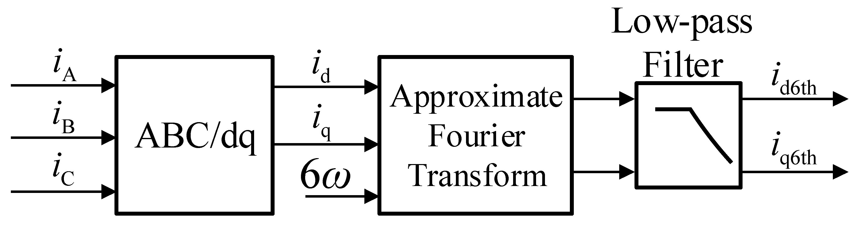
In a PMSM, frequencies of both the fundamental and harmonics are proportional to the rotor speed, so the desired harmonic frequency can be obtained online. The block diagram of harmonic estimator is shown in Figure 8, which can extract the 6th-order component of current in the synchronous reference frame.

3.2. Suppressing Harmonic Currents Using a PI Regulator

The extracted current harmonics by approximate Fourier transform can be directly used in the proposed compensation method. From Equations (4) and (5), it is sufficient to consider only the dominant 6th-order harmonics and neglect the higher-order harmonics which have little impact on the inverter output voltage. This paper considers only the 6th-order harmonics in harmonic suppression.

According to the principles of the linear system, subtracting Equation (1) from Equation (13) gives the harmonic voltage equation:

$$\{\begin{array}{l}{u}_{\mathrm{d}6\mathrm{th}}=R_{\mathrm{s}}{i}_{\mathrm{d}6\mathrm{th}}+L_{\mathrm{d}}\frac{d{i}_{\mathrm{d}6\mathrm{th}}}{dt}-{\omega }_{\mathrm{r}}{L}_{\mathrm{q}}{i}_{\mathrm{q}6\mathrm{th}}\\ u_{\mathrm{q}6\mathrm{th}}=R_{\mathrm{s}}{i}_{\mathrm{q}6\mathrm{th}}+L_{\mathrm{q}}\frac{d{i}_{\mathrm{q}6\mathrm{th}}}{\mathrm{d}t}+{\omega }_{\mathrm{r}}{L}_{\mathrm{d}}{i}_{\mathrm{d}6\mathrm{th}}\end{array}$$

(20)

In Equation (20), both the voltages and currents are AC. If we apply approximate Fourier transform to the 6th-order component of voltages and currents, then the harmonics are transformed to DC. A typical PI regulator is adopted to effectively following the 6th-order harmonic current command $i_{\mathrm{d}6\mathrm{th}}^{*}$ and $i_{\mathrm{q}6\mathrm{th}}^{*}$ which are expected to be zero.

A feedback loop with a PI controller to suppress the current harmonics is built up based on the 6th-order harmonic voltage equations. It should be noted that the derivation is approximate because the fundamental voltage equations have coupling terms which are known as back electromotive force. Generally, a vector-controlled PMSM adopts a simple decoupling feed-forward control, i.e., $-{\omega }_{\mathrm{r}}{L}_{\mathrm{q}}{i}_{\mathrm{q}}$ in d-axis and ${\omega }_{\mathrm{r}}(L_{\mathrm{d}}{i}_{\mathrm{d}}+{\mathsf{\lambda }}_{\mathrm{f}})$ in q-axis, which guarantees that the model of PMSM is approximately linear. Moreover, the harmonic voltage Equation (20) also includes higher-order harmonics besides the 6th-order ones in practical system. Though the model is not accurate, it is a common practice in engineering application, for a classic PI regulator is robust enough to tolerate model error to a certain extent and achieve the control target. The control block diagram of the 6th-order harmonic suppression is shown in Figure 9. Terms such as $-{\omega }_{\mathrm{r}}{L}_{\mathrm{q}}{i}_{\mathrm{q}6\mathrm{th}}$ and ${\omega }_{\mathrm{r}}{L}_{\mathrm{d}}{i}_{\mathrm{d}6\mathrm{th}}$ can decouple the harmonic voltage equations in a similar way as the fundamental voltage equations.

The feedback loop of the harmonic suppression requires the 6th-order harmonics to be transformed to DC, the error between the command value and the estimated one is the input of the PI regulator, as shown in Figure 9. The output of the PI regulator which is DC needs to be transformed to AC.

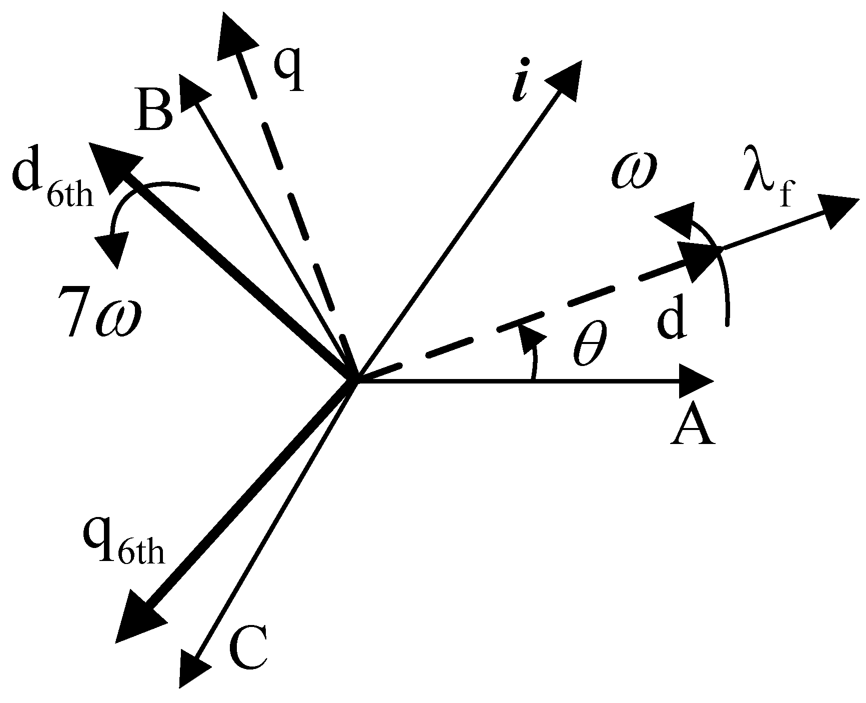
Imagine a frame $d{q}_{6\mathrm{th}}$ rotates at the same speed as the 6th-order harmonic vector, as shown in Figure 10, then the 6th-order harmonic in the frame is transformed to DC, while other components are AC.

According to the Park transform, the transform matrix between dq frame and $d{q}_{6\mathrm{th}}$ frame are given as:

$$C_{\mathrm{dq}6\mathrm{th}/\mathrm{dq}}=\left[\begin{array}{cc}\cos (6\theta )& -\sin (6\theta )\\ \sin (6\theta )& \cos (6\theta )\end{array}\right]$$

(21)

$$C_{\mathrm{dq}/\mathrm{dq}6\mathrm{th}}=\left[\begin{array}{cc}\cos (6\theta )& \sin (6\theta )\\ -\sin (6\theta )& \cos (6\theta )\end{array}\right]=C_{\mathrm{dq}6\mathrm{th}/\mathrm{dq}}^{-1}$$

(22)

Appling the transform in Equation (21) to the output of the harmonic PI regulator gives the AC value. The overall scheme to compensate for the nonlinearity of the inverter is shown in Figure 11, in which a current harmonic suppression controller is the core of the algorithm. In the PMSM, the dashed block indicates the part of the proposed compensation algorithm, while other blocks compose a typical vector control. The demand torque determines the demand currents $i_{\mathrm{d}}^{*}$ and $i_{\mathrm{q}}^{*}$, which are used to calculate the fundamental reference voltages $u_{\mathrm{d}}$ and $u_{\mathrm{q}}$. Harmonic suppression controller gives the compensating voltages which are added to the reference voltages to create rectified reference voltages $u_{\mathrm{d}}^{*}$ and $u_{\mathrm{q}}^{*}$.

4. Simulation of the Compensation Algorithm

Simulation using a model based on MATLAB/Simulink (version R2013b, MathWorks, Natick, MA, USA) was conducted in order to confirm the effectiveness of the proposed method. The specification of the PMSM with a three-phase PWM VSI is listed in

Table 1. Specification of the permanent magnet synchronous motor (PMSM).

Parameters	Value	Parameters	Value
Armature Resistance Rs (Ω)	0.092	DC voltage Vdc (V)	380
Magnetic flux in the d-axis (Wb)	0.202	Switching frequency fPWM (kHz)	5
Maximum speed (r/min)	10,300	Turn-on time ton (μs)	1
Maximum power (kW)	80	Turn-off time toff (μs)	2
Maximum torque (Nm)	205	Dead time td (μs)	5
d-axis inductance Ld (mH)	2.8	voltage drop of IGBTs vs (V)	3
q-axis inductance Lq (mH)	8.3	forward voltage of diodes vD (V)	2

.

In the first simulation, the PMSM operates at 270 r/min (18 Hz) and a load of 12.1 Nm which equals to the driving force of the whole vehicle.

In Figure 12a, phase currents are not pure sine waves and severely distorted due to the nonlinearity of the inverter. When one phase current crosses zero, it changes slowly and almost stays constant; the other two phase currents are also affected at the same time. An evident platform appears in each current waveform; this phenomenon is called zero-current clamping. The longer the platform lasts, the more distorted the phase current is and the more harmonics there are. Phase currents are less distorted after applying the compensation method, and waveforms are more close to sine waves, as shown in Figure 12b.

The spectra of phase current by fast Fourier transform (FFT) shows the magnitude difference of the sixth harmonic components in Figure 13. At motor speed of 270 rpm, the fundamental frequency of phase current is 18 Hz, and the frequencies of the fifth and seventh are 90 Hz and 126 Hz, respectively. The amplitudes of the fifth and seventh harmonic components in phase currents are 1.039 A and 0.8775 A, respectively. After applying the compensation method, amplitudes of the two harmonic components are 0.5233 A and 0.5989 A, which decrease by 46.20% and 31.78%, respectively. As the fifth- and seventh-order are the dominant harmonic components, the suppressing of the fifth and the seventh harmonics undoubtedly reduces the overall harmonic components in phase currents.

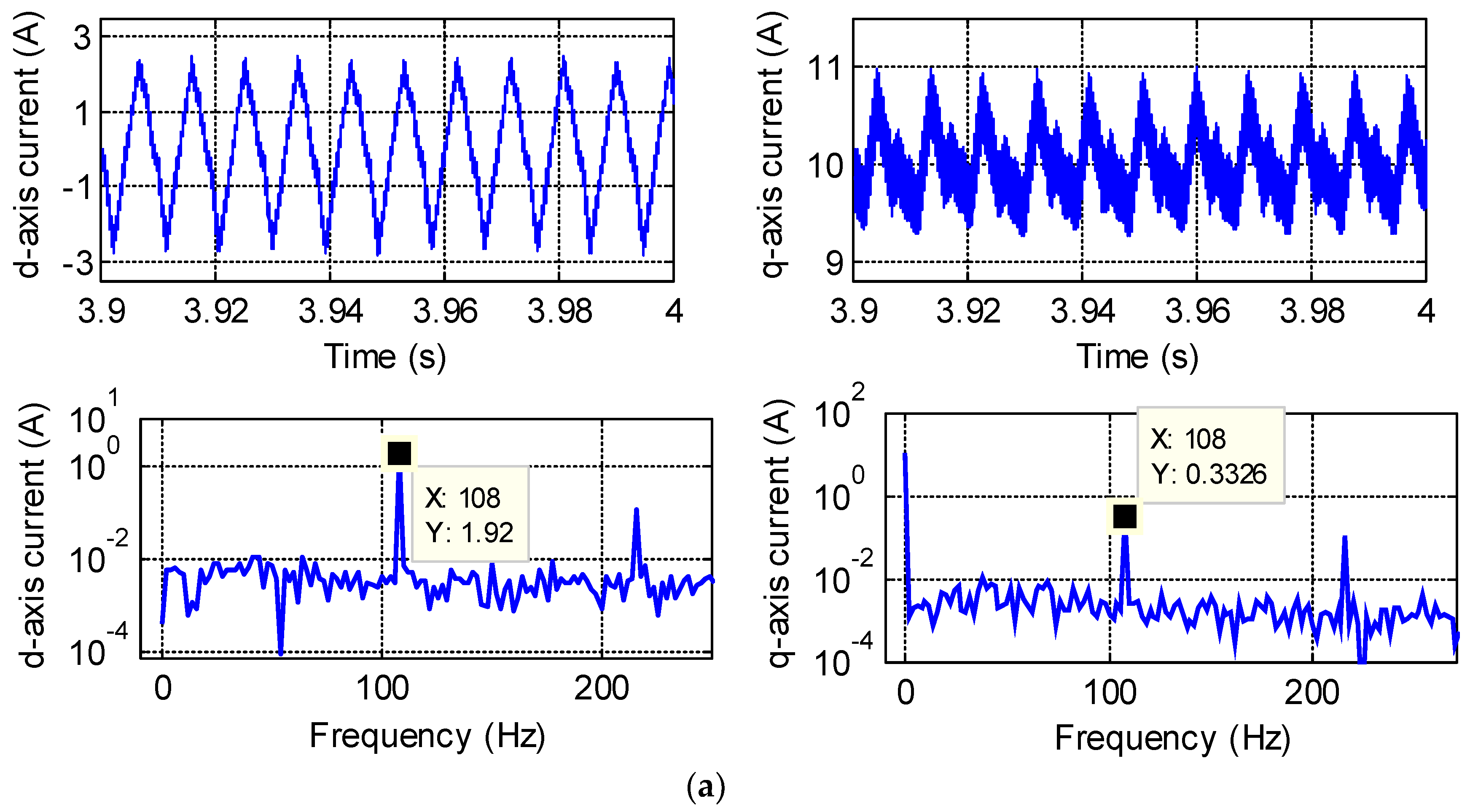
As described in Section 2, the fifth and seventh harmonics in phase currents correspond to the sixth harmonics in d-axis and q-axis currents. The ripples in both d-axis and q-axis currents reduce after applying the compensation method, indicating that the harmonic components caused by the nonlinearity of the inverter are suppressed. As shown in Figure 14, the amplitudes of the sixth harmonic components in d-axis currents are 1.92 A and 1.122 A before and after the compensation, respectively, reducing by 41.67%. The amplitudes of the sixth harmonic components in q-axis currents are 0.3326 A and 0.1712 A before and after the compensation, respectively, reducing by 48.8%.

In conclusion, the dominant harmonics in d-axis and q-axis currents caused by the nonlinearity of the inverter are reduced significantly.

Motor torque ripples reduce after applying the compensation method. According to torque Equation (15), the sixth harmonics in currents give rise to the sixth-order ripples in motor torque, as shown in the FFT results of motor torque in Figure 15. The amplitude of the sixth-order torque ripples is suppressed by 28.3% after applying the compensation method, from 1.206 Nm to 0.8603 Nm. The dominating sixth-order components in torque ripple decrease considerably.

The simulation waveforms before and after the compensation when the motor operates at 1920 r/min (768 Hz) and a load of 14.1 Nm are shown in Figure 16, Figure 17 and Figure 18.

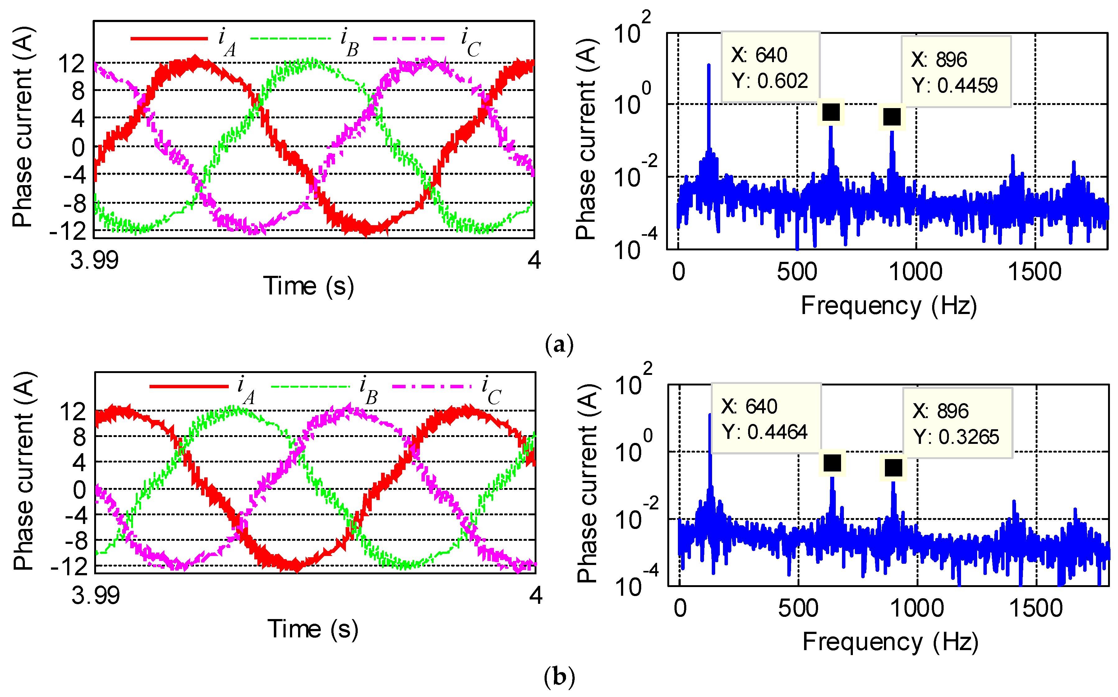
In Figure 16, the amplitudes of the fifth and seventh harmonic components in phase currents are 0.602 A and 0.4459 A, respectively. After applying the compensation method, the amplitudes of the two harmonic components are 0.4464 A and 0.3265 A, which decrease by 25.25% and 26.78%, respectively.

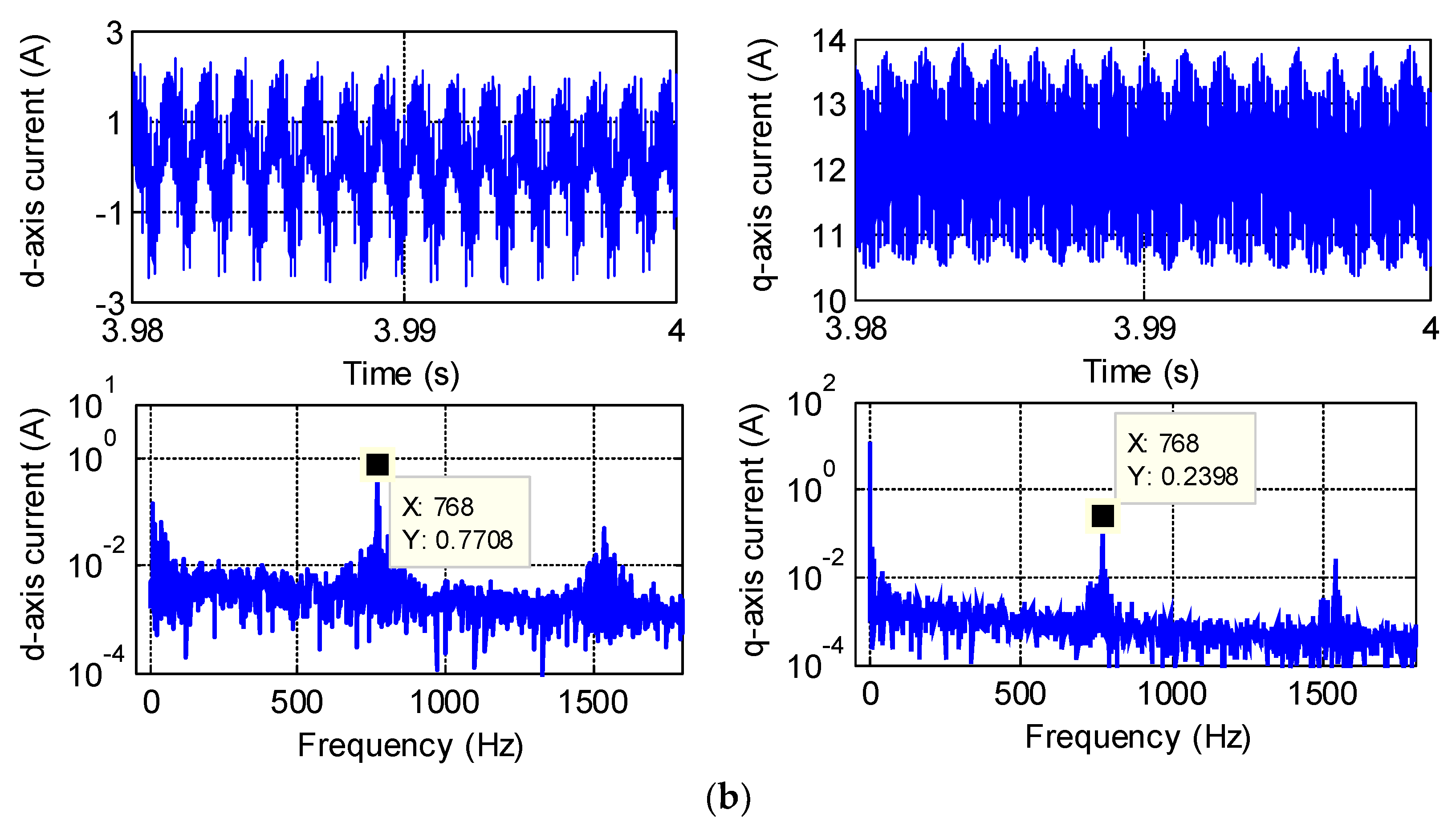
In Figure 17, the amplitudes of the sixth harmonic components in d-axis currents are 1.047 A and 0.7708 A before and after the compensation, respectively, reducing by 25.41%. The amplitudes of the sixth harmonic components in q-axis currents are 0.3132 A and 0.2398 A before and after the compensation, respectively, reducing by 23.44%.

In Figure 18, the amplitude of the sixth-order torque ripples is suppressed by 26.64% after applying the compensation method, from 0.8855 Nm to 0.6504 Nm.

According to the simulation results, it can be concluded that the 6th-order torque ripples are smoothed by suppressing the harmonic components in currents. However, there are still small parts of the 6th-order torque ripples remaining after applying the compensation method and two probable reasons are as follows. First, practical switching devices have limited switching frequency, i.e., they have finite response time, which may cause phase lag of output voltage. Moreover, voltage drops inevitably exist in switching devices and diodes. Consequently, there are errors between the compensating voltage output via the actual inverter and the one calculated by the algorithm. Second, harmonic voltage equations are derived based on the linear theory. However, the model of the PMSM has coupling terms and is not strictly linear, which causes model error in harmonic voltage equations.

The compensation method can suppress the dominant torque ripples caused by the nonlinearity of the inverter. Since the motor is the major excitation source of the torsional vibration of the electric vehicle powertrain, the influence on the torsional vibration after the torque ripple suppressing is studied in the next Section.

5. Analysis of the Powertrain Torsional Vibration Response

The configuration of the powertrain of a front-wheel drive electric vehicle is shown schematically in Figure 19. The drive motor is a PMSM. The vehicle control module determines the torque command according to the vehicle parameters such as the accelerator pedal position, the vehicle speed and the state of charge of the lithium-ion battery. The PMSM provides the torque according to the torque command.

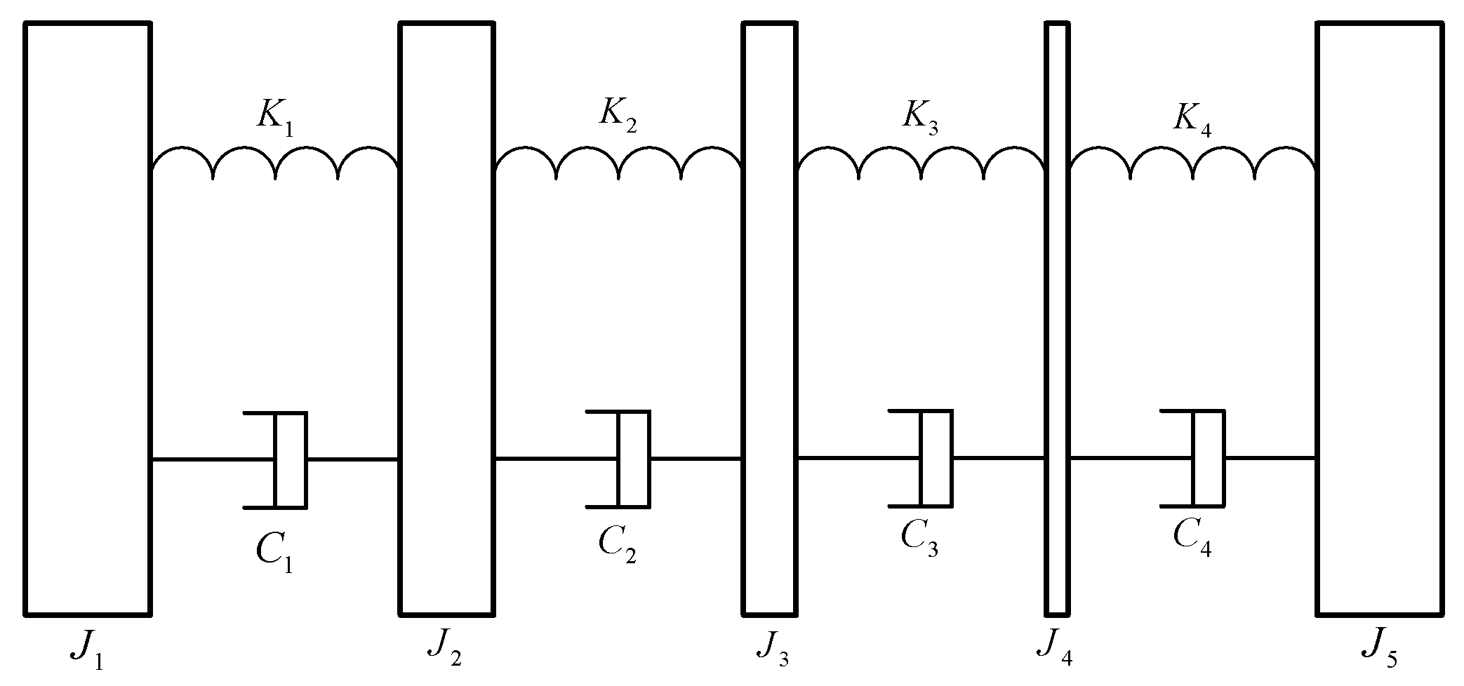
In order to analyze the torsional response of the system, a 5-DOF lumped parameter linear time invariant (LTI) mathematical model is built, as shown in Figure 20. The assumptions used in developing this model include:

• Rotor is modeled as a single lumped body with input excitations on it.
• For linearity, the backlash effects of the reducer and planetary gears are not considered.

Table 2. Inertia moments in the driveline model.

$J_1$	Inertia of rotor and half of the motor’s output shaft
$J_2$	Effective inertia of half of the motor’s output shaft, the input gear pairs of reducer and half of the middle shaft of the reducer
$J_3$	Effective inertia of half of the middle shaft of the reducer, the output gear pairs of the reducer, differential and half of the axles
$J_4$	Effective inertia of half of the axles and drive wheels
$J_5$	Effective inertia of the vehicle

and

Table 3. Torsional stiffness and viscous damping in the driveline model.

$K_1$ and $C_1$	Effective stiffness and viscous damping of motor’s output shaft
$K_2$ and $C_2$	Effective stiffness and viscous damping of middle shaft of reducer
$K_3$ and $C_3$	Effective stiffness and viscous damping of axles
$K_4$ and $C_4$	Effective stiffness and viscous damping of wheels

show the parameters in the model.

The equation of the motion of the torsional system can be written in matrix form as:

$$\mathit{J}\ddot{\mathit{\theta }}+\mathit{C}\dot{\mathit{\theta }}+\mathit{K}\mathit{\theta }=\mathit{T}$$

(23)

where $\mathit{J}$ is the inertia matrix, $\mathit{C}$ is the viscous damping matrix, $\mathit{K}$ is the stiffness matrix, $\mathit{\theta }$ is the rotational displacement vector and $\mathit{T}$ is the torque excitation vector. The abovementioned matrices can be written as:

$$\mathit{J}=diag[J_1{J}_2{J}_3{J}_4{J}_5]$$

(24)

$$\mathit{\theta }={[{\theta }_1{\theta }_2{\theta }_3{\theta }_4{\theta }_5]}^{\mathrm{T}}$$

(25)

$$\mathit{T}={[T_{\mathrm{m}}000-T_L]}^{\mathrm{T}}$$

(26)

$$\mathit{C}=\left[\begin{array}{ccccc}{\mathrm{C}}_1& -{\mathrm{C}}_2& & & \\ -{\mathrm{C}}_1& {\mathrm{C}}_1+{\mathrm{C}}_2& -{\mathrm{C}}_2& \mathbf{0}& \\ & -{\mathrm{C}}_2& {\mathrm{C}}_2+{\mathrm{C}}_3& -{\mathrm{C}}_3& \\ & \mathbf{0}& -{\mathrm{C}}_3& {\mathrm{C}}_3+{\mathrm{C}}_4& -{\mathrm{C}}_4\\ & & & -{\mathrm{C}}_4& {\mathrm{C}}_4\end{array}\right]$$

(27)

$$\mathit{K}=\left[\begin{array}{ccccc}{\mathrm{K}}_1& -{\mathrm{K}}_2& & & \\ -{\mathrm{K}}_1& {\mathrm{K}}_1+{\mathrm{K}}_2& -{\mathrm{K}}_2& \mathbf{0}& \\ & -{\mathrm{K}}_2& {\mathrm{K}}_2+{\mathrm{K}}_3& -{\mathrm{K}}_3& \\ & \mathbf{0}& -{\mathrm{K}}_3& {\mathrm{K}}_3+{\mathrm{K}}_4& -{\mathrm{K}}_4\\ & & & -{\mathrm{K}}_4& {\mathrm{K}}_4\end{array}\right]$$

(28)

where $T_{\mathrm{m}}$ is the motor torque and $T_L$ is the resistance torque of driving.

According to Equation (23), neglecting damping and excitation terms gives the equation of motion governing the free vibration response as:

$$\mathit{J}\ddot{\mathit{\theta }}+\mathit{K}\mathit{\theta }=\mathbf{0}$$

(29)

Free vibration of the driveline system can be computed by using the above equation, which includes natural frequencies and corresponding mode shapes, as shown in Figure 21.

Torsional mode characteristics are obtained from Figure 21 as follows. Mode 1 is the surge mode shape at 6.3 Hz where the vehicle body has the largest rotational displacement amplitude. Mode 2 is at 31.7 Hz where the wheels have the largest amplitude. There exists no vibration node in the driveline components in the two mode shapes above, so the resonant response in the driveline is low and can be neglected.

Mode 3, mode 4, and mode 5 of the driveline are at 333.7 Hz, 740 Hz, and 1210 Hz, respectively. Each of these three modes has at least one vibration node in the driveline components, and could cause higher resonance response at the motor’s output shaft and the middle shaft of the reducer. In the three modes, the displacement of the vehicle body is almost zero, while driveline components have relatively high displacement, so high-frequency excitations may cause severe torsional response in the driveline components, such as dynamic torque response of shafts.

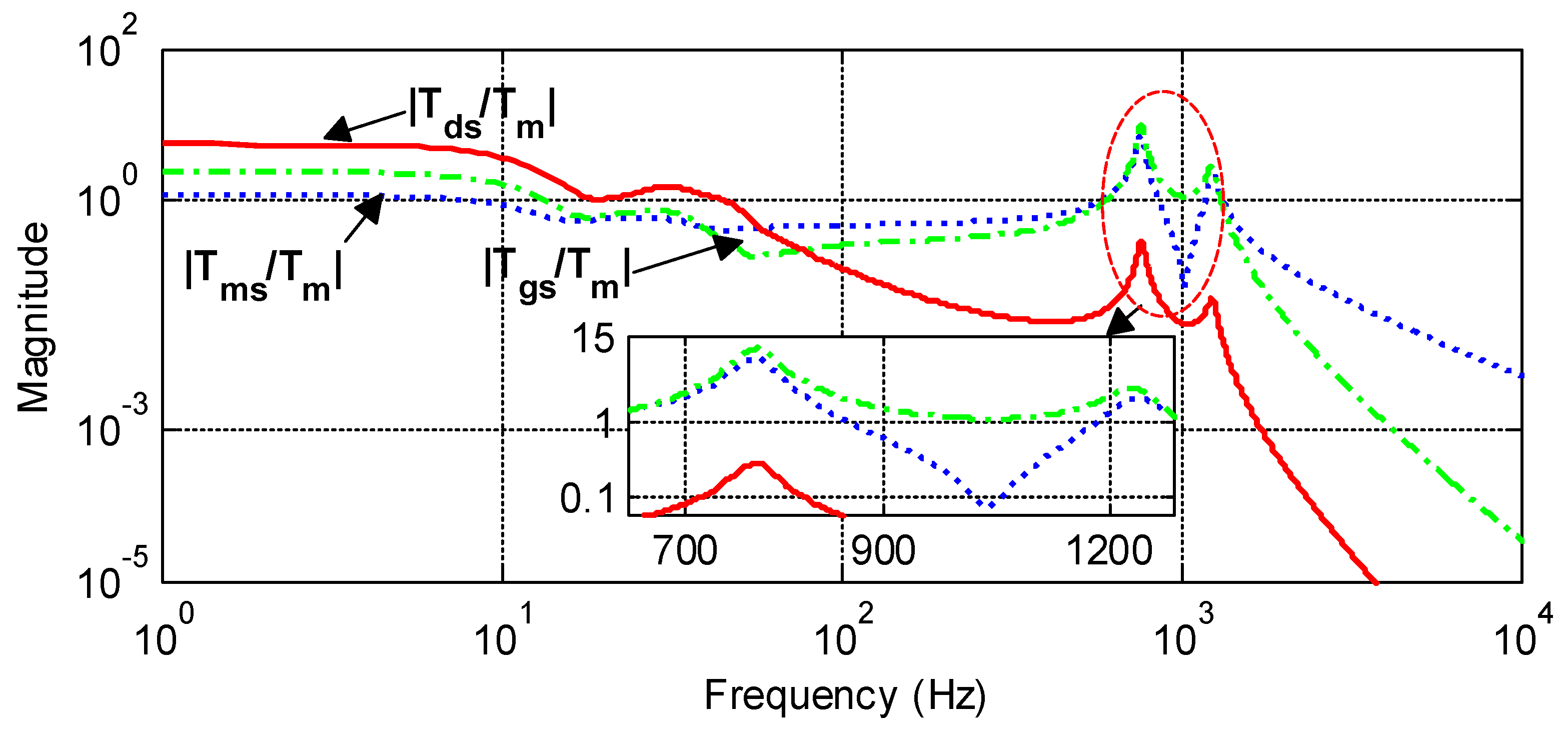
Frequency response of driveline component can be used to analyze the amplitudes and frequencies of resonance response in forced vibration. With motor torque as excitation and torque of driveline component as output, the torque response in frequency domain is given as shown in Figure 22. Angular velocity response of driveline components is obtained in a similar way, as shown in Figure 23. $T_{\mathrm{ms}}$, $T_{\mathrm{gs}}$ and $T_{\mathrm{ds}}$ are the torque of motor’s output shaft, middle shaft of reducer and axles, respectively. ${\mathrm{w}}_{\mathrm{m}}$, ${\mathrm{w}}_{\mathrm{g}1}$, ${\mathrm{w}}_{\mathrm{g}2}$ and ${\mathrm{w}}_{\mathrm{wheel}}$ are the angular velocity of rotor, input gear of reducer, output gear of reducer and wheels, respectively.

As shown in Figure 22, the amplitudes are obviously higher at 768 Hz and 1240 Hz. The two resonant frequencies are close to the natural frequencies of mode 4 and mode 5, which are 740 Hz and 1210 Hz, respectively. The slight differences between resonant frequencies and natural frequencies are due to viscous damping of the driveline. Torsional amplitudes in different resonant zones vary dramatically, which reveals that not all the resonant torsional vibrations cause severe response. The amplitudes of resonance response of motor’s output shaft are 7.45 and 2.16 at 768 Hz and 1240 Hz, respectively.

For the middle shaft of the reducer, the amplitudes of torsional response reach 10.13 and 2.58 at 768 Hz and 1240 Hz, respectively. It is observed that 10.13 is the largest among all torsional amplitudes of the driveline components, indicating that torsional vibration of the middle shaft of the reducer is the severest in the driveline. This is in good agreement with the analysis of mode 4 and mode 5 in Figure 21. Torsional amplitudes of torque response in the non-resonant zones, including both low-frequency and high-frequency zones, are low and can be ignored.

In Figure 23, compared with the torque response, the amplitudes of angular velocity response of driveline components are much lower, since the inertia of driveline components filter the high-frequency excitations.

The above analysis of free vibration reveals the behavior of forced vibration, such as resonant frequencies and corresponding torsional amplitudes. However, forced vibration of the driveline is not only affected by the driveline configuration which determines the free vibration, but also by the characteristic of excitations, especially the orders and amplitudes of harmonics in the excitations. In this paper, motor torque ripples caused by the nonlinearity of the inverter are the main excitations of the driveline torsional vibration in forced vibration. When an EV runs at a constant speed, the average motor torque is equal to the resistant torque of driving, which defines the steady state of the torsional vibration. At the steady state, torque ripples excite the driveline to vibrate continuously, while the average torque does not contribute to the torsional vibration. As described in Section 4, motor torque ripples decrease after implementing the compensation method for the nonlinearity of the inverter. The reduction in the torque ripples which are the major excitations of driveline affects the behavior of the forced vibration.

For evaluating the torque response in the time domain, the driveline is excited with the torque ripples generated by the motor. The motor torque ripples as excitations at 270 rpm and 1920 rpm, which correspond to the vehicle speed of 3.6 km/h and 26.0 km/h, respectively, are shown in Figure 15 and Figure 18.

According to the FFT results of motor ripples at rotor speed of 270 rpm in Figure 15, the frequency of the dominating 6th-order torque ripples is 108 Hz; 108 Hz is much smaller than the resonant frequencies which are 768 Hz and 1240 Hz. The case of 270 rpm rotor speed is used to investigate the torsional vibration excited by the harmonic torque components in the non-resonant zone.

According to the FFT results of motor ripples at rotor speed of 1920 rpm in Figure 18, the frequency of the dominating 6th-order torque ripples is 768 Hz; 768 Hz is equal to one of the resonant frequencies. Especially, the torsional amplitude of the reducer shaft is the biggest at 768 Hz. Therefore, the case of 1920 rpm rotor speed is used to investigate the torsional vibration excited by the harmonic torque components in the resonant zone.

The two typical motor speeds are used to analyze the steady-state time domain torsional response. The dynamic torque response of the middle shaft of the reducer is taken as an example, for its torsional vibration is the severest in the driveline. The steady-state time domain torsional response of torque at the middle shaft of the reducer is shown in Figure 24 and Figure 25, which also include the spectrum of dynamic torques obtained with FFT.

Figure 24 shows that, at motor speed of 270 rpm, the response of the middle shaft of the reducer is low, and the ripples only account for about 3% of the average torque before suppression. According to the torsional response in frequency domain, the frequency of the dominating harmonic component is 108 Hz, which is the same as the dominating harmonic order of the motor torque ripples. FFT results are in good agreement with the characteristics of the forced vibration, i.e., the response and the excitation have the same harmonic components.

The amplitudes of the dominating 6th-order torque response are 0.6478 Nm and 0.4621 Nm before and after suppressing the motor torque ripples caused by the nonlinearity of the inverter, the reduction is 28.67%. After implementing the compensation method for the nonlinearity of the inverter, the variation in the amplitudes of the 6th-order torque response is approximately the same as that of the 6th-order ripples in motor torque as 28.3%. It is clearly concluded that the reduction in the torsional response is achieved by suppressing the dominating 6th-order motor torque ripples caused by the nonlinearity of the inverter. However, for the middle shaft of the reducer at motor speed of 270 rpm, even before suppression, the amplitude of the dominating 6th-order harmonic component of the torsional response accounts for less than 10% of the average torque, as shown in Figure 15. Obviously, the torsional response in the non-resonant zone is quite small.

Figure 25 shows that, at motor speed of 1920 rpm, the steady torque response of the middle shaft of the reducer is obviously higher than that of 270 rpm, for the torque ripples account for about 30% of the average torque before suppression. The amplitudes of the dominant 6th-order torque response are 8.082 Nm and 5.924 Nm before and after suppressing motor torque ripples caused by the nonlinearity of the inverter, the reduction is 26.51%. Compared with the 6th-order ripples in motor torque, the amplitude of the 6th-order torque response is magnified 9.1 times, because the frequency (768 Hz) of the 6th-order harmonic components of motor torque at 1920 rpm is close to the frequency (740 Hz) of mode 4 of the driveline. After implementing the compensation method for the nonlinearity of the inverter, the reduction of the amplitude of the 6th-order torque response is about the same as that of the 6th-order ripples in motor torque as 26.64%.

For the middle shaft of the reducer at 1920 rpm, the amplitude of the dominating 6th-order harmonic component of the torsional response accounts for 30.3% and 22.3% of the average torque before and after suppressing the motor torque ripples, respectively. It is clearly concluded that the reduction in torsional response is achieved by suppressing the dominating 6th-order motor torque ripples caused by the nonlinearity of the inverter. Obviously, the torsional response in resonant zone is much higher than the response in the non-resonant zone even after the motor torque ripples has been suppressed.

Analysis of the steady response of other driveline components shows the similar results which are not presented in the paper for simplification.

From the steady torsional response results, by compensation for the nonlinearity of the inverter, the dominant 6th-order ripples in both motor torque and torsional response decrease by 26–28% in the overall motor operating range.

6. Conclusions

Harmonics in currents resulting from the nonlinearity of the inverter generate torque ripples in PMSM, and eventually cause torsional vibration in the driveline of an EV. This paper proposes a compensation algorithm for the nonlinearity of the inverter. The algorithm includes an estimator of the harmonic components in currents, and a harmonic current PI regulator to suppress the harmonic component. Decrease in torque ripples of the PMSM is achieved by suppressing the harmonics component in currents. The effectiveness of the proposed method is validated by simulation with MATLAB/Simulink. Simulation results show that the dominating 6th-order ripples in motor torque is reduced by approximately 26–28%. After implementing the compensation method, the dominating 6th-order in torsional response of the driveline excited by motor torque reduced about 26–28% as well.

Future research will focus on applying the proposed method to a real system. Identifying model parameters of PMSM such as d-axis and q-axis inductance is an inevitable issue then and the parameter variation sensitivity of the proposed method is to be investigated.